Alma Mater Studiorum – Università di Bologna
DOTTORATO DI RICERCA IN
Scienze e Tecnologie Agrarie, Ambientali e Alimentari
Ciclo XXX
Settore Concorsuale di afferenza: 07/E1 Settore Scientifico disciplinare:AGR/07
High-throughput phenotyping for the genetic dissection of drought tolerance
related traits in Zea mays and Triticum durum Desf.
Tesi presentata da: Dott. Giuseppe Sciara Coordinatore Dottorato: Chiar.mo Prof. Giovanni Dinelli
Relatore: Chiar.mo Prof Silvio Salvi Correlatori: Chiar.mo Prof. Roberto Tuberosa Dott. Marco Maccaferri
Table of Contents
1. Introduction ... 1
1.1. Cereals in the world ... 1
1.2. Gene, genotype, genome - phene, phenotype, phenome ... 2
1.3. A brief overview on crop genetic improvement ... 2
2. High throughput phenotyping of a maize introgression library for water use efficiency and growth-related traits ... 1
2.1. Introduction ... 1
2.2. Materials and methods ... 2
2.3. Results ... 6
2.4. Discussion ... 9
2.5. Conclusions ... 12
2.6. Tables and figures ... 13
3. Morphological characterization of a durum wheat association panel for root and shoot traits in a high-throughput phenotyping platform ... 29
3.1. Introduction ... 29
3.2. Materials and methods ... 36
3.3. Results ... 41
3.4. Discussion ... 45
3.5. Conclusions ... 49
3.6. Tables and figures ... 50
4. General considerations and perspectives ... 70
Bibliografy ... 71
1. Introduction
1.1. Cereals in the world
Cereals are the main staple food in human diet and livestock feeding. Indeed, out of 1.4 billion of hectares of cultivated land, almost a half (0.72 Mha) are used for cereal production (FAOSTAT, 2014). Almost 89% of world cereal production is from three main crops: maize (Zea mays), wheat (Triticum spp.) and rice (Oryza spp.). In the last 57 years, global wheat and rice production increased of more than 300% while maize production increased of almost five folds. This astounding result are not the consequence of higher land investments but rather of constant yield increase. This has been possible thank to a parallel development of agronomical practices and genetic improvement. At the same time, the proportion of peoples living under the hungry threshold moved from 30% to 10%. This none withstanding, malnutrition is still the main cause of death in the world with more than 668 million of people still living without an adequate nutrients intake, especially in Africa and Asia (Alderman et al., 2006; Mayer et al., 2008; Müller and Krawinkel, 2005). As consequence of that, United Nations declared sustainable food safety as one of the major goals of the humanity in the next future (https://sustainabledevelopment.un.org). Various factors hinder the reaching of such an ambitious goal. First, the global population will keep increasing at least until the 2050 until it will reach nine or ten billion individuals. Secondly, the parallel growth of per-capita income will cause a corresponding increase in per-capita food consumption (Tester and Langridge, 2010b). Last but not least, anthropic activity will severely impact the climatic equilibrium of the planet, with consequences which might be catastrophic. The global agro-system will have to respond to a more and more intense food demand in climatic conditions totally different from those of the last century. Droughts, floods and extremely high temperature will hit the planet with a frequency and strength never observed before (Mickelbart et al., 2015). Is therefore crucial that research focuses on those mechanisms which might guarantee a better resilience of the plants to such extreme conditions. Furthermore, this must be reached by reducing at the same time the agricultural environmental footprint. Given their role in human nutrition, this is particularly urgent for cereals. In this dissertation we will focus on the genetic and phenotypical dissection of those traits that are involved in drought tolerance mechanisms in durum wheat and maize. In particular, we will expose the results of two research conducted using high-throughput phenotyping techniques with the aim of discovery the genetic bases underling drought adaptive traits.
1.2. Gene, genotype, genome - phene, phenotype, phenome
When referred to cultivated species, genetic improvement refers to all those voluntary or involuntary, conscious or unconscious strategies that humans have used to adapt plants to different growing environments and/or uses. In agriculture, genetic improvement has two goals: or to increase the amount of good produced per resource unit (yield, productivity, stability, sustainability…) or to ameliorate the suitability of the goods to the consumption chain (qualities) (Poehlman, 1987).
From domestication to our days, genetic improvement has been essentially a two-step procedure: in the first step, we observe or measure one or more properties of individuals belonging to a certain population; in the second step, we destine to reproduction those individuals that, because of their superior ranking in the properties we are interested in, have more chances to produce a progeny superior to the population they come from. In order to be inheritable and therefore subjectable to genetic improvements, traits should have a genetic determinism; such traits are referred as phenes; the global set of phenes is usually referred as phenome. The set of phenes that functionally and or morphologically allow to distinguish between individuals of the same population is referred as phenotype (Fiorani and Schurr, 2013; Mahner and Kary, 1997). Phenotypes which are considered optimal for a certain scope are defined as ideotypes. Parallelly to phene, phenome and phenotype we could define gene, genome and genotype. Genes are parts of nucleic acids able to produce functional molecules. The genome is the set of genes plus non-coding and regulatory regions of the DNA. Genotypes are sets of molecular features of the DNA which allow to distinguish between individuals of the same population (Mahner and Kary, 1997). Having this said, we can summarize that genetic improvement is the process that, by manipulating the genotype, makes the phenotype more similar to the ideotype.
1.3. A brief overview on crop genetic improvement
Since there is a bi-univocal correspondence between genotype and phenotype, genetic improvement might be achieved both selecting phenotypes, selecting genotypes or both. Since domestication up to the second half of the XX century, genetic improvement was solely guided by phenotypic selection (Tester and Langridge, 2010b). Despite breeding history underwent dramatic changes in the way populations were constituted and the ideotypes inspiring the selection, the criteria used by humans to select the best individuals was exclusively the direct observation or measurement of phenes; since the modification of phenotypes is the goal of any genetic improvement effort, this strategy is theoretically the most solid; indeed, as long as the progeny is cultivated in the same environment and under the same management conditions of
their parentals, select the parentals with best phenotypes will guarantee a progeny with the best possible phenotypes. The limits of phenotypic selection came to the surface in the XIX century, when genetic improvement of crops started to be scientifically executed. Indeed, selection began to be performed in experimental stations where many individuals were evaluated in experimental conditions. Progeny of selected individuals, after multiplication, was cultivated in areas other than those where the selection was performed. This caused the phenotypic selection for target traits, chiefly yield and quality, to lack predictivity. The reason of that is basically that yield and, to a certain extent, qualities, are complex traits resulting from the complex interaction of simpler phenes. Phenes expression could either be beneficial, neutral or detrimental for a complex trait depending on environment and management conditions. E.g. resistance to a certain disease has no impact on yield in those environments where the disease is absent while it is advantageous under strong disease pressure. Another example is deep rooting: it might be advantageous in drought scenarios (if soils are deep and a deep water-plane is available) while, in well-watered conditions, it might just be a waste of carbon.
The lack of predictivity of direct phenotypic selection for yield and qualities, caused ideotypes and phenotypes to include more and more phenes, each of which functionally involved in the resulting complex trait. One of the direct consequences of this approach was the more and more frequent – and successful – adoption of intraspecific hybridization for the constitution of breeding population (Borojevic and Borojevic, 2005b; Salvi et al., 2013; Scarascia Mugnozza, 2005). Indeed, to introduce a desired phene into the cultivated elite material, breeders begun to cross it with exotic germplasm which, despite it was not valuable from an agronomical standpoint, was carrier of few useful phenes. The impact of such approach has been tremendous. The pioneering work of Nazareno Strampelli in the early XX century is a glaring example of the successes obtained by phene manipulation (Salvi et al., 2013; Scarascia Mugnozza, 2005). Italian wheat breeding at the Strampelli’s time was facing three major challenges:
1. adapt wheat to new farming conditions established after the introduction of ammonium fertilization in agriculture;
2. reduce the dramatic yield reduction due to terminal drought; 3. improve leaf rust resistance;
Strampelli is the first scientist who obtained to adapt wheat to the fertility boost due to the introduction of ammonium fertilization in agriculture. One of the major constrain to ammonium fertilization was indeed the lodging phenomenon, overcame by Strampelli introducing in the elite “Rieti originario” derived material, dwarfing alleles of the Rht8 gene from Japanese local variety “Akakomugi” (Borojevic and Borojevic, 2005a, 2005b). The same cross allowed Strampelli to
introgress the early variant of the ppd-D1 gene producing a sensible reduction in flowering time (Salvi et al., 2013). This allowed, by reducing the length of the wheat cycle, to plummet the risk of droughts during flowering/grain filling, especially in Mediterranean climates. Finally the introduction of the resistant variant of the Lr34 (Kolmer et al., 2008; Lagudah et al., 2009) gene, conferred good levels of resistance to leaf rust. Three decades later, the Nobel laureate Norman Borlaug used the Strampelli’s lines and strategy to constitute the lines of the green revolution. The progressive introgression of favorable alleles in the elite germplasm is one of the crucial factors that permitted the crops productivity to increase of more than 300%. Introgression of favorable alleles into the elite germplasm has several limitations that pushed breeders, physiologists and geneticists to develop strategies more and more sophisticated. One of the major constrain for phenes manipulation is for sure the limited, if not null, variability in terms of alleles affecting phenes in the desired direction. Different approaches have been used to enrich germplasm of potentially beneficial alleles. The first attempts in this direction have been through physical and chemical mutagenesis (D’Amato et al., 1962; Neuffer and Ficsor, 1963; Oladosu et al., 2016; Shama Rao and Sears, 1964). These techniques cause random changes in the DNA both at sequence or structure level. Most of the mutations occur in neither genic or regulatory regions of the DNA thus having no phenotypic consequences. In the case mutations occur in functional genomic regions, they might cause aminoacidic change and, therefore, changes in the protein which might in turn cause phenotypic variation. The International Atomic Energy Agency (IAEA), reports in its databases (https://mvd.iaea.org/) over 3200 cultivars of 232 species developed using one of the following mutagenesis-based breeding techniques:
1. direct use of a mutant line obtained after physical or chemical mutagenesis 2. use of a mutant as parent in crosses
3. use of a mutant allele
4. irradiation-facilitated translocation of genes from wild ancestors to elite germplasm. Rice is by far the specie with more mutagenesis-breeding derived cultivar (821), followed by barley (304), chrysanthemum (281), wheat (255) and soybean (173). The same database reports a total of 31 durum wheat cultivar released after the use of one of the above-mentioned strategies. Being mutations randomly distributed in the genome, many individuals are needed to have good chances that at least one of them carry an ameliorative mutation. Furthermore, both physical and chemical mutagenesis cause mutations in numerous loci in the genome with possible negative effects on other phenes. These two aspects represent strong limitations to the effective employment of mutagenesis in breeding. Another major limiting factor is the fact that through mutagenesis it is not possible to tune gene expression levels.
Parallelly to mutagenesis, the development of genomics and biotechnologies marked the beginning of a new era in breeding. The use of biotechnologies in genetic improvement has had two major finalities: i) to enrich natural genetic variation, ii) to enhance selection efficiency by integration of phenotypic and genotypic information. Biotechnologies started to impact plant breeding as soon as genetic transformation through Agrobacterium was developed (Bevan et al., 1983; Herrera-Estrella et al., 1983; Parmar et al., 2017). This strategy permits the stable integration of genetic material from any species into the genome of a recipient species. Individuals which genome was enriched by mean of this technology are commonly referred as Genetically Modified (GM). Classic examples of GM uses are the incorporation in vegetal genomes of bacterial toxins from Bacillus thuringiensis to obtain insect resistant crops or the artificial enhancement or introgression of biosynthetic pathways to produce bio-fortified food i.e. “Golden rice” (Mayer et al., 2008; Sanahuja et al., 2011). Other biotechnological tools that allow the direct modification of the genetic pool of plants are referred as genome editing (GE) techniques. The most important family of these techniques is that of site direct nucleases (SDNs). SDNs permit the precise cut of a specific genomic region; they can either be DNA-binding restriction proteins able to recognize, bind and cut in a certain position of the genome (meganuclease) or heterodimers of two proteins having one the function to recognize the genomic region and the other to cause the actual cut. Zinc finger nucleases (ZFNs) and transcription activator‐like effector nucleases (TALENs) are two representative examples of this technology. These proteins are usually coupled with Fok1, which cause the actual cut of the DNA. In order to permit the editing to occur, is therefore needed that two genes encoding for the above-mentioned proteins are expressed in the cells. SDNs could be used for single point mutation, insertions or deletions of entire gene or genomic regions (D’Halluin et al., 2013; Osakabe et al., 2010; Petolino et al., 2010; Shukla et al., 2009; Townsend et al., 2009). In the last few years, an innovative technology is emerged which, because of its precision and ease of use, promises to revolutionize the impact of GE in plant breeding. This technology is named CRISPR/Cas9 and is a SDN where the Cas9 nuclease is directed to the target genomic region by an ad hoc designed RNA guide (Barrangou et al., 2007; Cai et al., 2018; Jinek et al., 2012; Wang et al., 2017; Zhou et al., 2016).
Despite the above-mentioned biotechnological tools permit a much more accurate control of genetic modification as compared to mutagenesis, their application in breeding has faced several constrains which have strongly limited their wide diffusion. First of all, they need long and costly development for the discovery, modification and patenting of the genes to insert or modify; secondly, in several developed countries, especially in Europe, they found an harsh opposition by large part of the public opinion because of often unfounded safety concerns which translates;
finally, because they permit the modification of a relatively low number of loci thus being unsuitable for the improvement of very complex traits such yield or most of stresses tolerances (Hartung and Schiemann, 2014; Tester and Langridge, 2010a).
As above mentioned, biotechnologies have not only allowed for the enrichment of genetic variability of germplasms but also they have been used to increase selection predictivity accuracy in breeding. The main use of biotechnologies in this direction is commonly referred as marker assisted selection (MAS). MAS fundamentally take advantage of detectable variation (molecular markers) present in the DNA sequence to track and monitor specific regions of the genomes during crossing and selection (Moose and Mumm, 2008). Because of linkage disequilibrium, markers might be predictive of the allelic status of the genetically linked loci. Those loci where one or more genes are involved in the control of a quantitative trait are referred as quantitative trait
loci (QTLs). The allelic status at a certain marker linked to a QTL might therefore be predictive of
a certain phenotype. MAS consists in the integration of phenotype-based selection with genotype information at critical loci. Mas is especially useful when the target traits have low heritability, the costs of phenotyping are high or if breeders are interested to introgress in elite material just a small part of the genome of a wild relative (i.e. backcrosses). Molecular markers are also crucial in gene cloning, the process that permits the identification of the gene causally controlling a certain phene (Salvi and Tuberosa, 2005). MAS has not faced the same ostracism as other biotech tools. Furthermore, it permits to contemporary track the entire genome and thus to be particulary suitable to complex traits breeding (Tester and Langridge, 2010b) In order to develop markers suitable for MAS, is crucial to identify those QTL controlling the target trait. The QTL discovery strategies are fundamentally statistical regressions where is tested the significance of the association between measured phenes values of a relatively high number of individuals and their genotypic information. As above mentioned, many stresses tolerance mechanisms, notably drought, have a complex genetic and phenotypic architecture. Is therefore crucial to dissect tolerance into component contributory phenes and to identify QTLs controlling them (Araus et al., 2002; Langridge and Reynolds, 2015; Tuberosa, 2012). The high number of individuals needed for QTL discovery jointly with the numerosity of phenes to be collected to dissect complex traits is the origin of what is known as the phenotyping bottleneck (Fiorani and Schurr, 2013; Furbank and Tester, 2011). High throughput phenotyping is the set of technologies developed to permit to obtain with adequate accuracy many phenes on QTL discovery suitable populations.
In the next chapters, we will present two researches where, by use of high throughput phenotyping, we have been able to identify several loci involved in drought tolerance-related phenes in maize and durum wheat.
growth-related traits
2. High throughput phenotyping of a maize
introgression library for water use efficiency and
growth-related traits
2.1. Introduction
Water deficit is one of the major factors limiting crop yield potential. Despite this, the genetic basis of drought tolerance remains mostly unknown because of its intrinsic complexity. Modern breeding approaches try to tackle the complexity of drought tolerance first by dissecting it into simpler secondary traits by means of eco-physiological modelling (Abdel-Ghani et al., 2016; Reynolds and Langridge, 2016; Salvi et al., 2011; Szalma et al., 2007; Wei et al., 2015). Each secondary trait is supposed to have a simpler genetic control than yield under drought and, therefore, to be more easily manipulated by breeding. For instance, plant geneticists and physiologists focused on traits such as stomatal conductance, leaf water status and/or osmotic potential, root anatomy and architecture and others (Roy et al., 2011; Vadez et al., 2013).
The capability of plants to uptake water and maintain water use (WU) together with their capability of efficiently use it (water use Efficiency, WUE, defined as the amount of water needed to produce a certain amount of biomass) have been recognized as key components of drought tolerance (Blum, 2009; Reynolds and Tuberosa, 2008; Richards and Passioura, 1989). Several approaches permit to directly or indirectly estimate WUE both at field and plant levels. Despite just a part of the total biomass produced is finally harvested, biomass accumulation rate (BA) in specific growth phases (e.g. early vegetative growth) can be critical for the plant to successfully address later phases such as flowering, fertilization and grain filling. Furthermore, being leaves the main organ of the plant deputed to gas exchange with atmosphere, their extension, together with stomatal density and control, is critical to determine plant water consumption.
One of the major hurdles in working with secondary traits is that their phenotyping can be more time consuming and less repeatable than directly measuring yield. This limitation will likely be mitigated by the advent of high-throughput phenotyping technologies, which appear as particularly suitable for the dissection of abiotic stress tolerance. (Araus and Cairns, 2014; Cabrera-Bosquet et al., 2012; Reynolds et al., 2009; Tuberosa, 2012). One of the advantages of these technologies is the possibility to perform morpho-physiological measurements dynamically, thus enabling to study traits which are usually inaccessible to phenotyping based on single time point (or end-point) measurements.
Several types of populations have been conceptualized and developed to perform phenotype/genotype associations. Among them, introgression libraries (ILs, also referred to as chromosomal substitution lines), allow for the evaluation of chromosomal regions from a donor parent (DP) into a common genetic background from a recurrent parent (RP) (Zamir, 2001). This approach is especially useful for the exploitation of genetic diversity originating from exotic or unadapted plant materials. Indeed, the DP is usually chosen because of the presence of interesting traits despite its overall inadequacy to common farming conditions. On the contrary, the RP is usually a well-characterized highly productive elite line or genotype. Multiple introgression libraries have already been generated in maize (Abdel-Ghani et al., 2016; Salvi et al., 2011; Szalma et al., 2007; Wei et al., 2015).
In this experiment, we used a high-throughput phenotyping strategy to evaluate drought tolerance related traits in a maize IL previously found to segregate for phenology and root system architecture (RSA) (Salvi et al., 2011, 2016). The phenotyping platform PhenoArch (https://www6.montpellier.inra.fr/lepse_eng/M3P/PHENOARCH-platform) is a conveyer based system which permit the dynamic, non-destructive evaluation of biomass and WU and thus to have a direct estimation of WUE (Cabrera-Bosquet et al., 2016; Coupel-Ledru et al., 2014; Lopez et al., 2015). Furthermore, its design allowed for an accurate control of soil water status and atmospheric parameters such as temperature, relative humidity and photoperiod, thus permitting an accurate evaluation of the plant response to water deficit.
We aimed to test whether genetic variation for phenology and RSA would affect BA and WU during the early phase of development, in an elite maize genetic background.
2.2. Materials and methods
Plant material and genetic characterization
A total of 73 lines from a previously developed introgression library (IL) population (Salvi et al., 2011) plus the two parents were tested. The RP of the IL was the elite dent line B73, an inbred line also used as reference for sequencing the maize genome (Schnable et al., 2009) while the DP was the early-flowering north American flint landrace Gaspé Flint (Vigouroux et al., 2008). The IL was obtained through five generation of SSR-marker-assisted backcross followed by two cycles of selfing (Salvi et al., 2011). The IL was previously found to segregate for phenology traits and seminal roots architecture (Salvi et al., 2011, 2016). In this work, the genetic characterization of the IL was refined in respect of the previously available data (Salvi et al, 2011) by means of the 50k SNP ILLUMINA Infinium array (Ganal et al., 2011). A total of 48,361 SNPs were utilized after excluding SNPs with unknown or unclear physical map position on the maize reference
growth-related traits genome (Schnable et al., 2009) and those with >10% of missing data. A graphical genotype of the IL was constructed by creating chromosome BINs of consecutive SNPs with identical genotypic score and labelling the BINs with the first SNP of the BIN. BINs of length < 200 kb and with < 5 SNPs were masked. Linkage Disequilibrium (LD) between BINs was evaluated using TASSEL 5 (Bradbury et al., 2007). LD p-values were estimated by a two-sided Fisher's Exact test (Fisher, 1922). Two BINs were considered in high LD when the calculated p-value was < 0.01.
Experimental design and traits evaluation
The high-throughput phenotyping platform PhenoArch is hosted in a greenhouse of the Laboratory of Plant Eco-physiology under Environmental Stresses (LEPSE) of the French Agricultural Research Institute (INRA) in Montpellier, France. The platform consists of 28 belt conveyers each of which can carry up to 60 pots, for a total throughput of 1680 pots/plants. Conveyers permit the automatic transport of the pots to both watering stations and imaging cabin. The platform hosts two automated watering stations consisting in balances with 1g accuracy (ST-Ex, Bizerba, Balingen, Germany) and high-precision pumps (520U, Watson Marlow, Wilmington, MA, USA). The imaging cabin is provided with two RGB camera (1280×960 px, 3D Scanalyzer, LemnaTec, GmbH, Wüerselen, Germany) and a rotating lift which permits the acquisition of lateral plant pictures from up to 12 angles (0° to 330° with 30° steps) plus a single picture from the top. Biomass was estimated by a four steps process consisting in: 1) image segmentation to isolate the plant from the background and thus estimate the number of pixels it was made of; 2) extrapolation, through image analysis of geometrical properties of the picture of the plants such as width, height, convex hull etc…; 3) selection, among the 12 lateral pictures, of the frontal one (where the plant had the maximum width); 4) estimation of fresh biomass (B) and leaf area (LA) on the base of the number of pixels of the plant in the frontal and the top pictures by means of multiple linear models previously calibrated using destructive measurements. Air temperature, relative humidity and VPD was monitored in eight spots of the greenhouse. Day and night air temperature was maintained at 24 and 18 °C respectively. Natural lighting was integrated with HPS lamps light in order to impose a 18/6-hour (light/dark) photoperiod. Plants where grown in cylindrical pots (55x15 cm) filled with peat-based compost. Pots were weighted twice per day in order to evaluate soil water content and thus, on the base of a previously estimated soil water retention curve, soil water potential. Plants were subjected to two soil water status: well-watered (WW) and water deficit (WD). In WW, soil water potential was maintained at >1 MPa; in WD, irrigation was suspended when the population was averagely at the 8th leaf stage. When soil water potential was less of the target threshold of -4 MPa, each pot was irrigated dispensing the exact amount of water needed to bring the soil water potential back to -4 MPa. The experimental unit
consisted in a single pot where a single plant was grown. Per each water treatment, eight randomized replicates of the entire IL population and the two parents were grown up to the 13th leaf stage. A lattice design was used to avoid the neighbouring of two replicates of the same genotype.
Thermal Time (TT) was estimated for WW and WD as 20 °C equivalent days as previously suggested (Parent et al., 2010). All time-related traits will be reported as referred to TT. As mentioned above, PhenoArch allows for two classes of automated measurements: ponderal (twice per day) and imaging (once every two days at night). Growth curves for biomass and leaf area were fitted using the package grofit (Kahm et al., 2010) in the statistical software R (The R Core Team, 2016). Three possible fitting models were evaluated: logistic, Gompertz, modified Gompertz and
Richards (Zwietering et al., 1990). For each pot, the model with lower Akaike Information Criterion
(AIC) was choose (Akaike, 1974). Ponderal measurements were took twice per day; each time the weight of the plant plus the pot and the tutor was measured immediately before and after watering. The amount of water evapo-transpired (ET) between two consecutive measurement was estimated as follow:
𝐸𝑇 = 𝑊𝑎𝑖−1− 𝑊𝑏𝑖− ∆𝐵
Where:
𝑊𝑏𝑖 is the weight of the pot plus the plant before watering at the ith measurement
𝑊𝑎𝑖−1 is the weight of the plant plus the pot after watering at the measurement preceding the ith ∆𝐵 is the increase in biomass between the two measurements.
In order to obtain comparable observations, we analysed the traits just in an evaluation time window between the imposition of the final target soil humidity in WD and the harvest. Rate of Biomass Accumulation (BA) was calculated as the biomass increase between the start and the end of the evaluation window divided for the TT elapsed. Daily Water Use (WU) was estimated as the total amount of water evapo-transpired during the evaluation window and its duration expressed in TT. Water Use Efficiency (WUE) was estimated as the total biomass increase in the evaluation window and the total amount of evapo-transpired water in the same time. Specific Transpiration (T) was calculated as the average amount of water used between two phenotyping points and the average LA of the plant during the same interval. Early Vigor (EV) was measured as estimated fresh biomass before the water deprivation treatment (~ 8th leaf stage). BA, WU and T response to water deficit (BA_res, WU_res and T_res) were calculated as the ratio between the standardized phenotypic values of each trait in WW and WD.
growth-related traits The number of visible leaves was scored visually twice per week. An additional score was given to the last visible leaf according to its stage of development as follows:
0.3 – leaf visible just inside the previous leaf sheath 0.5 – leaf blade just emerged the previous one sheath 0.8 – leaf blade fully visible and mostly expanded.
Leaf number was calculated as the number of visible leaves plus the last visible leaf score. Linear fitting was then performed between leaf number and thermal time. We refer to the slope of this fitting as phyllochron (Phy). Thus, Phy approximates the number of leaves emitted per thermal day. Since WD affected Phy and just three scores were available in the evaluation period, the results relatives to Phy are referred to the only WW plants.
Micro-environmental effect estimation
In order to evaluate the effects of the micro-environmental variation on the observed traits, a two-step strategy was adopted. First, for each trait the difference from the genotypic mean was calculated for each pot within the experimental design; secondly the micro-environmental effect of the XY position was calculated as the average of the difference of the pots surrounding the XY position. Outliers were detected using the Dixon’s Q test (Dixon, 1951) and excluded from further analysis.
Statistical analysis and QTL detection
Statistical analysis was performed using the software R (The R Core Team, 2016). All the graphics and plots were made using the ggplot2 package (Wickham, 2009). Two-tailed correlation tests were performed using the package psych v. 1.6.7 (Revelle, 2017) and the obtained p-values corrected according to Benjamini and Hockenberg (Hochberg and Benjamini, 1990) for false discovery rate. Correlation between traits measured in this experiment and experiments previously conducted on the same materials, were calculated on the BLUPs value of each line calculated by means of the
lme4 package (Bates et al., 2015) using the variable “Genotype” as the only random variable and
no other fixed-effect variate. Principal Component Analysis (PCA) was performed on scaled values using the princomp function of the stats package (The R Core Team, 2016). Dunnett’s multiple comparison test was carried out using the package multcomp (Dunnett, 1955; Hothorn et al., 2008). Broad sense heritability (h2) was calculated using the function repeatability of the package
repeatability (Wolak et al., 2012). The genetic position of the markers was assigned according to the
nearest marker on the reference map “Genetics” (Coe et al., 2002). Single BIN QTL analysis was performed by t-test comparison between the lines carrying the given introgression and the lines
without the same introgression, and correcting the resulting p-values accordingly to Bonferroni (Bonferroni, 1936). We herein define QTL clusters those BINs or groups of BINs in strong LD (Fisher test p-value < 0.01) that showed evidence of trait-genotype association (p-value Bonferroni corrected <0.01) for at least two traits. In case of genetically linked QTL, QTL were considered as distinct in case of contrasting direction of genetic effect of the donor fragment.
2.3. Results
Effect of water regimes on vegetative growth and water use
The two water regimes (well-watered: WW and water deficit: WD) strongly influenced Biomass accumulation (BA), Daily water use (WU), Transpiration rate (T) and Water use efficiency (WUE), with a reduction of 69%, 46%, 42% and 44%, respectively (Fig. 1; Table 1) in the WD treatment. As an exemplification of the data type and quality collected in this experiment, the time-course (per day) change of BA in the two water regimes for all B73 pots is shown in Fig. 2.
Phy was measured in well-watered plants only. Early vigor (EV) was measured before starting the water deprivation period therefore no response to water regimes was made available. Trait repeatability (h2) was overall acceptable ranging 0.50 - 0.59 for BA, WU and WUE, and 0.38-0.39 for T (Table 1). EV and Phy showed h2 values of 0.53 and 0.62, respectively (Table 1).
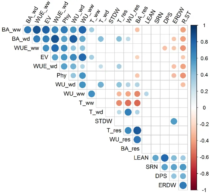
Correlation among traits
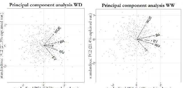
BA, EV, WU, WUE and Phy were positively correlated in both WW and WD conditions (Fig. 4; Table 2). Instead, T generally showed weaker correlation values, with the only significant values observed between T_wd and WU_wd (r = 0.33) and with T_ww negatively correlated with BA_res and WU_res (r = -0.39 and -0.48, respectively). The three ‘response to water deficit traits’ (BA_res, T_res and WU_res) resulted positively correlated (r values from 0.58 to 0.82. P < 0.001), as expected given their physiological connection (ie. water deprivation is expected to impact in the same negative direction on the three traits). A PCA-based multivariate analysis of platform trait variation showed that the first two principal components (PC1 and 2) explained >80% of total variability (Fig. 3). Overall, vectors for traits collected in platform clustered in a comparable manner in WW and WD. In WW, PC1 was the result of similar loadings assigned to all the five platform traits while PC2 was mainly the result of positive load of WUE and negative load of T. In WD conditions, PC1 had the same composition observed for WW while PC2 mainly showed a contribution from WUE (positive loadings) and EV (negative loadings).
Correlations between platform traits with other morpho-physiological traits collected on the same IL lines in previous experiments (Salvi et al. 2011 and 2016) were also computed. Concerning
growth-related traits root traits, it is interesting to note that Root/Shoot ratio (R/ST) was negatively correlated with BA, EV, WU, WUE and Phy in both WW and WD conditions (r ranging from -0.19 to -0.45. Table 2) while its components (Embryonal Roots Dry Weight and Shoot Dry Weight, ERDWT and STDW, respectively) were not. Phenology-related traits evaluated in the field (Leaf Number and Days to Pollen Shed, LEAN and DPS respectively), showed little correlation with platform traits, except for mild correlations observed between LEAN and WU_ww (r = 0.30, P < 0.05) and between DPS and WUE_ww (r = -0.28, P <0.05).
Water use efficiency and response to water stress of IL lines
In our experiment, the two main components of WUE (BA and WU) were independently assessed, which provided the opportunity to explore physiological and genetic mechanisms responsible for WUE variation .
In WW, 18 IL lines showed higher WUE than B73 and just one line showed lower WUE (Table 3). For the ‘high WUEww’ lines, higher WUE was associated to higher BA coupled with significant difference for WU (seven lines), a significant increase in BA coupled with a non-significant reduction of WU (three lines) or an increase of both BA and WU but with a proportionally higher increase in BA (eight lines). The only IL line (IL38) with lower WUE in WW also showed lower WUE in WD; additionally, IL38 showed significantly lower values of WU in both water conditions, and lower BA and Phy, overall suggesting a developmental weakness likely caused by the homozygosity of low performance GF allele(s) not necessarily linked with water balance traits.
In WD, seven lines were characterized by WUE higher than B73 and six by lower WUE. Among the seven with higher WUE, six lines had high WUE associated with either much higher BA matched with unchanged WU (++BA & =WU. IL56, 60, 66 and 72) or by a slightly higher BA matched with a slightly lower WU (+BA & −WU. IL57 and 67. Table 3). The same six lines showed WUE higher than B73 in WW too. However, the seventh line (IL63) showed higher WUE than B73 at WD only. This line reached higher WUE than B73 by reducing WU (−26.99 g; P < 0.01. Dunnet test vs. B73, corrected for multiple tests) without affecting BA accumulation (Table 3). For IL63, a marginally significant reduction of WU was observed in WW too, however this reduction was not enough to impact on WUE in WW. Finally, IL63 showed a negative water use response to water deficit treatment (WU_res < 0. P < 0.001) while did not show any negative response on BA accumulation (BA_res ≈ 0). The same line did not show any significant difference from B73 for other traits such as EV, Phyl and T. Overall, these results suggest that different mechanisms of plant water balance regulation are in place among the different IL lines.
QTL for plant growth-related traits, water use and water use efficiency
A total of 20 QTL clusters and 8 non-overlapping QTL were detected in eight out of ten chromosomes confirming the complex genetic control of the nine physiological traits collected in platform (Fig. 5). Details on all QTL clusters composition and position, and single QTL position, effect, proportion of variance explained and statistical significance are reported in Table 4 also includes QTL for total number of leaf (LEAN), days to pollen shed (DPS), root to shoot ratio (R.ST), embryonic root dry weight (ERDW) and number of seminal roots (SRN) recomputed here using previously collected phenotypes (Salvi et al. 2011, Salvi et al. 2016) and the new 50k-SNP genotype matrix.
Overall, QTL for the tightly physiologically related traits BA, WU, and WUE showed a clear tendency to cluster, supporting the reliability of the results. Additionally, within the same cluster, QTL for these traits were characterized by highly concordant direction of genetic effect (eg. a positive BA genetic effect corresponded to a positive WUE genetic effect, as expected physiologically). In the following, when not specified, the QTL effect is discussed with reference to the Gaspé Flint (GF) allele.
At Q1 (bin 1.01-02) the GF allele increased BA, WU, and WUE in WW condition and WU in WD condition. Similarly, at Q4 (bin 2.01-02) the GF allele showed a positive effect on EV, WUE (both WW and WD), BA (in WD) and WU_res. Q4 was in long-range LD with Q3 on chromosome 1. At Q6 (bin 2.06-08) the GF introgression showed a strong negative effect on BAwd and EV, which likely negatively contributed to the concurrent negative effect on WUwd and WUEwd. This was also confirmed by the negative effect recorded for BA_res and WU_res.
At Q8 (chr. 3), the GF substitution had a negative effect on most traits (BA, EV, WU and WUE) in both WW and WS conditions. Accordingly, no effect was observed on responsive traits (BA_res and WU_res). Q8 encompassed a large portion of chromosome 2 (from 32 to 145 cM) due to the presence of very long GF chromosome introgressions and common introgressions among different IL lines.
The GF allele substitution at Q11 (bin 4.03) induced a strong positive effect on EV (+8.5 g, P < 1×10⁻⁴) and had the strongest effect on biomass accumulation throughout the whole experiment (Q11 BAww genetic effect: +3.97 g, P < 1×10⁻⁸). This effect likely drove the positive effect on WUEww and the negative effect on BA_res. It should be noticed that Q11 seemed to act at WW only and no effect was detected in WD on any of the traits.
Q15 mapped at the bottom of chr. 6 and showed a negative genetic effect on EV and WUwd. The
effect on EV was the strongest recorded in this experiment (−10.5 g, P = 6.4 × 10⁻⁹).
growth-related traits At Q17 (chr. 8), 19 (chr. 9) and Q20 (chr. 10) GF allele substitutions showed mostly positive effects on BAwd, EV, WUEwd, WUEww and others, with the exception of mild negative effect on WUww at Q17 only.
Phy QTL were mapped at four QTL clusters (Q8, Q12, Q17 and Q18) with positive and negative genetic effects. At Q8 (chr. 3), the GF allele reduced Phy rate (−0.011 leaf × thermal day−1. P = 3.6 × 10⁻⁵) in accordance with the negative effect recorded for all other traits at this QTL cluster. At Q12, Q17 and Q18, GF allele was associated with positive effects on Phy. Interestingly, at Q17, Phy QTL overlapped with the flowering time QTL Vgt1 and Vgt2, known to segregate between GF and B73 (Salvi et al. 2011); more precisely, at this QTL cluster the GF substitution increased Phy rate (0.007 leaf × thermal day−1. P = 9.3 × 10⁻³) while reducing the number of total nodes and number of days to flowering (Salvi et al. 2011. See Discussion).
2.4. Discussion
Correction for micro-environmental variability
Semi-controlled environments such as a greenhouse provide the possibility to grow plants in relatively ideal conditions strongly reducing the possibility that extreme or uncontrolled environmental events negatively affect the accuracy and repeatability of the experiment. The advanced PhenoArch system additionally allowed for accurate control of the soil water status. Nevertheless, micro-environmental variability was still detectable thus decreasing the heritability (repeatability) of the traits, if left unaccounted for. In order to address this problem, we have applied a correction method (fully explained in Materials and Methods). The method strongly increased h2 values especially for those traits (T and EV) with low h2 before the correction (Table 1). The main advantage of the proposed technique as compared to other methods is that it corrects for local non-random spatial effect not intercepted by other explanatory variables such as replicate, XY coordinate etc. Nevertheless, one of the limitation of the method is that while the spatial effect is limited to a specific position on the experimental grid, the moving replicates method extend the effect to the nearby positions owing to the limited number of plants for each moving rep, a problem that we partially addressed by discarding outliers from the moving rep prior to final analysis.
WUE was significantly lower in WD than in WW. This finding can be explained by the way the global evapo-transpiration was estimated. In this experiment, water was poured directly on soil surface hence the transpiration component of ET was affected similarly by the water treatment because evaporation was comparable between WW and WD conditions. Thus, the reduction in rate of biomass accumulation was proportionally higher than the reduction in evapo-transpiration,
resulting in lower WUE in the plants subjected to WD. Indeed, the reduction of BA and WU consequent to water deficit was equal to 69.6 and 46%, respectively while the reduction of WU was of just 46.0%.
Early vigor and its relationship with WUE
Given its importance in field performance and abiotic stress tolerance, genetic variation and control of early vigor in maize have been addressed in several studies (Hund et al., 2004; Jompuk et al., 2005; Liao et al., 2004; Presterl et al., 2007; Ruta et al., 2010; Trachsel et al., 2010, 2016). In our study, EV was one of the more strongly correlated traits with BA and WU in both water regimes. This is explained by the fact that early-vigor plants have also a larger canopy, which can better sustain plant growth. Positive correlation was also found with WUE in both water scenarios. The positive correlation with WUE can be explained by the fact that in plants with larger leaf area, the transpiration component tends to prevail on evaporation, thus reducing the role of water lost through evaporation. This is confirmed by the fact that eight out of eleven lines with significantly higher EV than B73, were more WUE in WW. By contrast, just three of the EV lines were among those more WUE in WD. QTL analysis allowed us to genetically localize the loci affecting EV. In this respect, QTL of EV and WUE often overlapped, like in the case of QTL cluster Q1 (chromosome 1, BIN1.1) characterized by higher EV (+6.89 g) and WUE (+0.01%) in WW only. A similar effect was detected for Q11 (chromosome 4, BIN 4.03). In the case of Q4 and Q19, EV was positively associated with WUE in both WW and WD. Given the high LD (p-value <0.01) between these two BINs in our population, it was not possible to map the QTL to a single BIN.
Root shoot ratio measured at seedling stage is negatively correlated with WUE
Several studies have shown the importance of seminal RSA on adaptive capability of plants to abiotic stresses (Bishopp and Lynch, 2015; Hochholdinger and Tuberosa, 2009). In this study we had the opportunity to evaluate a population which was previously characterized for some RSA traits (Salvi et al. 2016). In Figure 4 we report the phenotypic correlations between root traits collected by Salvi et al. by means of the paper roll technique and shoot growth traits collected in this experiment. Unexpectedly, no significant correlation was detected between shoot dry weight at seedling stage and growth components. On the other hand, significant correlations were found between root/shoot ratio and BA and WUE in WW; BA, WU and WUE in WD, other than with EV and Phy. Among the lines used in this experiment, two were found to have a higher R.ST than B73 and six a lower one. Only one of the latter lines showed significantly different EV as compared to the RP while half of them were different in terms of BA in WW and three out of
growth-related traits eight in WD. Interestingly, the embryonal root dry weight was negatively correlated with Phy and not with the other measured traits. These results indicate that those plants preferentially allocate more carbon to the shoot at seedling stage, maintain similar behaviour across the entire vegetative growth. This explains also the negative correlation found between R.ST and WUE: a more shoot-oriented allocation of metabolites resulted in improved shoot growth, water consumption made equal. This hypothesis seems to be confirmed by the colocalization of R.ST and WUE QTL in
Q1 and Q17, although the low genetic resolution of this experiment does not permit us to exclude
the action of linked but functionally distinct genes underlying the two traits. The confidence interval of Q1 indeed includes Rtcs, a gene previously characterized for its influence on RSA (Taramino et al., 2007) and already proposed as candidate for a QTL for number of seminal roots mapped in the same region (Salvi et al. 2016). Several QTL for RSA were also identified on the
Q17 region in different genetic backgrounds (Burton et al., 2014; Pestsova et al., 2016; Wu et al.,
2015; Zurek et al., 2015). This notwithstanding, a constitutively reduced allocation of photosyntates to the RSA might be detrimental in case of nutrient/water limited field conditions. Notably, yield QTL have been detected in the same region of Q1 in WW field conditions but not in WD (Millet et al., 2016).
Among the 73 IL lines, IL63 showed the higher WUE and could be considered an example of “conservative WUE” line. IL63 line showed lower WU and similar BA when compared to the RP (B73) in WD conditions. Interestingly, this line did not show lower T as compared to B73. IL63 carries a 27.2 cM Gaspé Flint introgression between the BINs 3.04 and 3.05 (69.8 cM – 97.03 cM of the Genetics reference map) and was previously shown to be early flowering when compared with B73 due to a major QTL, named Vgt3 (Salvi et al. 2011), similarly mapped in several independent experiments (Romay et al. 2013; Hirsch et al. 2014; Millet et al. 2016). Additionally, the same line develops a higher proportion of juvenile leaves (Salvi et al. 2011) which are characterized by a much higher leaf epicuticular wax than adult leaves ((Poethig, 1990; Vega et al., 2002). In IL63, transition occurs at leaf-10 rather than at leaf-7- 8 as in B73. Thus, the higher WUE of this line (and of the corresponding QTL) could be due to the fact that this line allocated less of its photosyntetates to canopy expansion than to other shoot sinks (e.g. stem, leaves thickness) thus maintaining low water use at the same time.
Flowering time genes and WUE
The IL lines studied in this experiment were formerly characterized for phenology traits such as DPS, LEAN and others (Salvi et al., 2011). Specifically, this population is known to segregate for
vgt1 and vgt2 (Bouchet et al., 2013; Chardon et al., 2005; Salvi et al., 2002) and these two strong
Flint allele shortened flowering time and increased WUE in both WW and WD, with a significant effect on BA in both conditions. It is also interesting to notice that within the QTL cluster Q17,
Vgt1 coincided with the peak of a Phy QTL (Bin 8.05, 104.6 - 138.2 Mb. Supp Tab. 2) where
Gaspé Flint again contributed for the positive effect allele (in this case, increaed pace of leaf emission). Additionally, a large GWA study recently identified a major flowering time QTL (SNP marker AX-91405380, 159.5 Mb) near but distinct from Vgt1, characterized by a positive effect on yield in many water regimes (Millet et al. 2017). A simple, although still speculative explanation is that vgt1 (or perhaps the combination of different flowering time QTL at bin 8.05-06, in strong LD in this population) might act on flowering time not only by affecting the time of transition of the apical meristem to the reproductive phase, but also by acting on the vegetative developmental pace (either plastochron or Phy, or both), providing the opportunity for the early-Gaspé Flint allele to accumulate more biomass per unit of time. The use of the PhenoArch platform was instrumental for the detection of the genetic effect on Phy.
2.5. Conclusions
This study identified and characterized several maize IL lines with well-defined contrasting physiological responses to water regimes, in the B73 elite genetic background, the most extensively investigated line in maize from genetic and physiological standpoints. For the first time, we observed a correlation between root/shoot ratio at seedling stage and WUE at full vegetative growth. Indeed, it seems that the tendency of certain genotypes to preferentially allocate resources to the shoot results in an increase in WUE, especially in WW conditions. In the case of QTL cluster Q1, the presence within the confidence interval of a strong candidate gene such as Rtcs could indicate it as candidate gene for the reduced root/shoot ratio. In the other case, further fine mapping efforts are needed in order to identify the causal genes. As regard to phenology traits, a QTL for delayed juvenile to adult transition was shown to affect WUE in WD conditions and it is possible that this association is linked to an augmented number of wax-coated juvenile leaves. Additionally, for the first time a significant effect of a major flowering time QTL (Vgt1) was detected on maize Phy, with the early flowering allele also contributing to faster Phy and thus positively affecting biomass accumulation and WUE. Although the presence of more than one introgression in the same IL line often limited the capability to accurately localize the QTL, this study provided clear evidence of the power of high-throughput phenomics investigation on well characterized elite genetic materials, towards the genetic dissection of physiological processes of agronomic impact such as plant response to water deficit.
2.6. Tables and figures
Table 1 Mean values of the observed traits for the entire population and the RP (B73) in both the experimental conditions. Broad sense heritability is reported both before and after the moving replicates correction.
Variable ID Variable description Unit Population average WW B73 WW Population average WD B73 WD H2 before correction WW H2 after correction WW H2 before correction WD H2 after correction WD BA Daily biomass accumulation g/20°C day 11.15 11.08 3.422 3.55 0.32 0.57 0.33 0.55
WU Daily water use g/20°C day 186.2 180.9 101.08 106.7 0.35 0.59 0.29 0.53
T Specific
transpiration rate g/m
220°C day 113.8 115.2 66.51 69.74 0.33 0.38 0.20 0.39
WUE Water use
efficiency g/g 0.0594 0.053 0.0335 0.0329 0.37 0.50 0.34 0.52
EV Early Vigor g 48.06 46.58 NA NA 0.22 0.53 NA NA
Phy Phyllochron Leaves/20°C day 0.27 0.27 NA NA 0.43 0.62 NA NA
BA_res BA response to water deficit Standard BA_ww/ Standard BA_wd NA NA 0.857 0.947 NA NA NA 0.40 WU_res WU response to water deficit Standard WU_ww/ Standard WU_wd NA NA 0.979 1.169 NA NA NA 0.57 T_res Transpirative response to water deficit Standard T_ww/ Standard T_wd NA NA 0.831 0.951 NA NA NA 0.47
Table 2 Correlation matrix reporting in the bottom left corner Pearson’s correlation among traits and in the top right corner significance of the correlation. Correlations between the following traits are reported: daily biomass accumulation (BA, g/20°C day), daily evapo-transpired water (WU, g/20°C day), early vigor measured as estimated fresh weight at eight leaves (EV, g), specific transpiration measured as WU per cm2 of leaf area(T, WU/cm2), water use efficiency, (WUE, BA/WU, g/g), Phyllochron (leaves emitted per 20 °C day). Suffixes “ww” and “wd” indicate whether the QTL was detected on well-watered or water deficit conditions respectively. Traits measured by Salvi et al. 2011 and Salvi et al. 2016 are reported as DPS (days per pollen shed), LEAN (leaf number), R.ST (root-shoot ratio, g/g), ERDW (embryonal root dry weight, g) and STDW (shoot dry weight, g).
WU_ww T_ww Phy WUE_ww BA_ww WU_wd T_wd WUE_ wd BA_wd WU_res BA_res T_res LEAN DPS ERDW STDW SRN R.ST EV WU_ww 1.00 *** *** *** *** *** * *** *** *** ** * *** T_ww 0.47 1.00 * *** ** *** Phy 0.61 0.01 1.00 *** *** ** *** *** * * * *** *** WUE_ww 0.41 0.03 0.63 1.00 *** ** *** *** * * *** *** BA_ww 0.80 0.26 0.71 0.87 1.00 *** *** *** * *** ** *** WU_wd 0.63 0.09 0.40 0.40 0.60 1.00 * *** *** * * * *** T_wd 0.03 0.33 -0.19 -0.03 -0.02 0.33 1.00 *** WUE_wd 0.30 -0.09 0.54 0.79 0.65 0.48 0.09 1.00 *** * ** *** BA_wd 0.52 0.02 0.54 0.70 0.73 0.83 0.25 0.88 1.00 ** *** WU_res -0.48 -0.48 -0.31 -0.12 -0.31 0.31 0.19 0.06 0.20 1.00 *** *** BA_res -0.41 -0.39 -0.30 -0.30 -0.41 0.28 0.26 0.17 0.26 0.82 1.00 *** T_res -0.36 -0.49 -0.18 -0.07 -0.24 0.23 0.64 0.14 0.21 0.62 0.58 1.00 LEAN 0.30 0.06 0.08 -0.24 0.01 0.14 0.16 -0.19 -0.05 -0.24 -0.09 0.06 1.00 *** ** *** ** DPS 0.18 0.08 -0.12 -0.28 -0.08 0.05 0.20 -0.22 -0.10 -0.22 -0.11 0.08 0.78 1.00 ** *** *** ERDW -0.07 0.11 -0.32 -0.28 -0.21 -0.16 0.16 -0.30 -0.27 -0.05 -0.01 0.03 0.43 0.39 1.00 *** *** *** STDW 0.15 0.12 0.10 0.16 0.21 0.15 0.06 0.08 0.13 0.03 -0.01 -0.07 0.08 -0.07 0.56 1.00 SRN 0.07 -0.03 -0.17 -0.14 -0.06 0.02 0.16 -0.01 0.00 -0.12 0.03 0.11 0.52 0.54 0.53 0.05 1.00 *** R.ST -0.19 0.04 -0.45 -0.45 -0.41 -0.31 0.15 -0.40 -0.41 -0.09 -0.02 0.10 0.37 0.48 0.71 -0.17 0.58 1.00 * EV 0.71 0.14 0.59 0.71 0.83 0.60 -0.03 0.64 0.73 -0.22 -0.21 -0.16 -0.04 -0.07 -0.21 0.07 0.02 -0.29 1.00
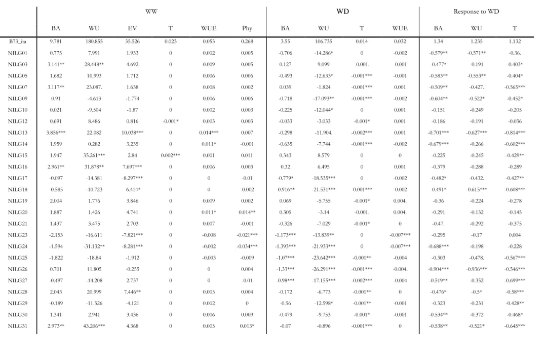
Table 3 Differences between the observed values of the IL lines vs. B73. Asterisks indicate significance levels calculated by the Dunnett’s multiple comparison test and indicate the following p-value: “*”≤ 0.05, “**” ≤ 0.01 and “***” ≤ 0.001
WW WD Response to WD
BA WU EV T WUE Phy BA WU T WUE BA WU T
B73_ita 9.781 180.855 35.526 0.023 0.053 0.268 3.55 106.735 0.014 0.032 1.34 1.235 1.132 NILG01 0.775 7.991 1.933 0 0.002 0.005 -0.706 -14.286* 0 -0.002 -0.579** -0.571** -0.36. NILG03 3.141** 28.448** 4.692 0 0.009 0.005 0.127 9.099 -0.001. -0.001 -0.477* -0.191 -0.403* NILG05 1.682 10.993 1.712 0 0.006 0.006 -0.493 -12.633* -0.001*** -0.001 -0.583** -0.553** -0.404* NILG07 3.117** 23.087. 1.638 0 0.008 0.002 0.039 -1.824 -0.001*** 0.001 -0.509** -0.427. -0.565*** NILG09 0.91 -4.613 -1.774 0 0.006 0.006 -0.718 -17.093** -0.001*** -0.002 -0.604** -0.522* -0.452* NILG10 0.021 -9.504 -1.87 0 0.002 0.003 -0.225 -12.044* 0 0.001 -0.151 -0.249 -0.205 NILG12 0.691 8.486 0.816 -0.001* 0.003 0.003 -0.033 -3.033 -0.001* 0.001 -0.186 -0.191 -0.036 NILG13 3.856*** 22.082 10.038*** 0 0.014*** 0.007 -0.298 -11.904. -0.002*** 0.001 -0.701*** -0.627*** -0.814*** NILG14 1.959 0.282 3.235 0 0.011* -0.001 -0.635 -7.744 -0.001*** -0.002 -0.679*** -0.266 -0.602*** NILG15 1.947 35.261*** 2.84 0.002*** 0.001 0.011 0.343 8.579 0 0 -0.225 -0.245 -0.429** NILG16 2.961** 31.878** 7.697*** 0 0.006 0.003 0.32 6.495 0 0.001 -0.379 -0.288 -0.289 NILG17 -0.097 -14.381 -8.297*** 0 0 -0.01 -0.779* -18.535*** 0 -0.002 -0.482* -0.432. -0.427** NILG18 -0.585 -10.723 -6.414* 0 0 -0.002 -0.916** -21.531*** -0.001*** -0.002 -0.491* -0.615*** -0.608*** NILG19 2.004 1.776 3.846 0 0.009 0.002 0.069 -5.755 -0.001* 0.004. -0.36 -0.224 -0.278 NILG20 1.887 1.426 4.741 0 0.011* 0.014** 0.305 -3.14 -0.001. 0.004. -0.291 -0.132 -0.145 NILG21 1.437 3.475 2.703 0 0.007 -0.001 -0.326 -7.029 -0.001* 0 -0.47. -0.292 -0.375 NILG23 -2.153 -16.611 -7.821*** 0 -0.008 -0.021*** -1.173*** -13.839** 0 -0.007*** -0.295 -0.17 0.004 NILG24 -1.594 -31.132** -8.281*** 0 -0.002 -0.034*** -1.393*** -21.933*** 0 -0.007*** -0.688*** -0.198 -0.228 NILG25 -1.822 -18.84 -1.912 0 -0.003 -0.009 -1.07*** -23.642*** -0.001** -0.004 -0.303 -0.478. -0.567*** NILG26 0.701 11.805 -0.255 0 0 0.004 -1.33*** -26.291*** -0.001*** -0.004. -0.904*** -0.936*** -0.546*** NILG27 -0.497 -14.208 2.737 0 0 -0.01 -0.98*** -17.155*** -0.002*** -0.004 -0.519** -0.352 -0.699*** NILG28 2.043 20.999 7.446** 0 0.005 0.004 -0.172 -6.773 -0.001** 0 -0.476* -0.5* -0.58*** NILG29 -0.189 -11.526 -4.121 0 0.002 0 -0.56 -12.598* -0.001** -0.001 -0.323 -0.231 -0.428** NILG30 1.341 2.941 3.436 0 0.006 0.009 -0.479 -9.753 -0.001* -0.001 -0.534** -0.372 -0.468* NILG31 2.973** 43.206*** 4.368 0 0.005 0.013* -0.07 -0.896 -0.001*** 0 -0.538** -0.521* -0.645***
WW WD Response to WD
BA WU EV T WUE Phy BA WU T WUE BA WU T
NILG32 3.06** 32.652*** 4.967 0 0.007 0.012. 0.058 3.221 0 0 -0.495** -0.367 -0.397* NILG34 3.278** 19.784 4.107 0 0.008 -0.001 0.125 4.517 0 0 -0.492* -0.193 -0.359. NILG37 -1.254 -16.439 -7.342** 0.001. -0.002 -0.02*** -0.874** -8.664 0 -0.006*** -0.295 0.067 -0.133 NILG38 -2.85** -32.345*** -13.596*** -0.002*** -0.013** -0.014* -0.904** -4.319 -0.002*** -0.006*** 0.493* 1.151*** -0.068 NILG40 1.116 26.523* 5.856* 0 0 0.007 0.254 -3.774 0 0.003 -0.1 -0.439 -0.321 NILG42 1.907 7.043 0.512 0 0.008 0.006 -0.159 -10.871 0 0.002 -0.494** -0.482* -0.339 NILG43 -0.172 6.839 1.63 0 -0.002 -0.009 0.072 -4.052 -0.001*** 0.001 -0.02 -0.25 -0.692*** NILG44 2.252. 9.308 5.689* 0 0.009. 0 0.608 5.423 0 0.003 -0.197 -0.036 -0.122 NILG45 1.665 6.94 -3.873 0 0.005 0.006 -0.395 -10.781 -0.001. 0 -0.533** -0.455* -0.434** NILG46 2.175 17.177 3.358 0 0.009 0.007 0.023 -1.572 0 0.001 -0.445. -0.318 -0.386* NILG47 2.849** 26.489* 2.321 0 0.007 0.013* 0.013 3.981 -0.001** 0 -0.49* -0.287 -0.459** NILG48 2.174 2.502 5.254 0 0.012** 0.012. 0.28 -1.349 -0.001** 0.003 -0.29 -0.093 -0.168 NILG49 3.891*** 30.512** 6.538* 0 0.012** 0.015** 0.299 5.61 -0.001 0.001 -0.453* -0.271 -0.317 NILG50 0.816 17.649 -1.348 0.001 0 0.008 -1.135*** -19.179*** -0.001** -0.005* -0.823*** -0.782*** -0.577*** NILG51 0.446 -19.915 1.793 -0.001 0.008 -0.005 -0.613 -19.259*** -0.001. 0 -0.477* -0.356 -0.022 NILG52 2.883** 14.859 5.386 0 0.01* 0.009 0.109 -2.437 0 0.002 -0.455 -0.312 -0.278 NILG53 1.734 13.149 0.38 0 0.009 -0.005 0.271 -3.666 -0.001* 0.004 -0.224 -0.241 -0.448** NILG54 -3.177*** -38.258*** -7.157** 0 -0.01. -0.034*** -1.128*** -16.088*** 0 -0.006*** 0.431. 0.701*** -0.161 NILG55 0.371 -1.821 -0.994 0 0.003 0.005 -0.393 -13.231* -0.001** 0.001 -0.421. -0.422 -0.328 NILG56 4.157*** -0.176 0.532 0 0.023*** 0.021** 0.866** 2.261 0 0.007*** -0.317 0.08 -0.386* NILG57 1.695 -6.893 1.752 0 0.015*** 0.009 0.222 -7.668 -0.001* 0.005** -0.241 -0.096 -0.097 NILG58 -0.989 -36.934*** -3.709 -0.001** 0.005 -0.003 -0.303 -13.204* -0.001*** 0 0.097 0.844*** 0.049 NILG59 3.243*** 9.968 3.388 0 0.014*** 0.019*** -0.31 -9.991 -0.002*** 0 -0.658*** -0.466* -0.731*** NILG60 2.991** -20.018 5.752 0 0.018*** 0.01 0.916** -0.782 -0.001. 0.006*** -0.023 0.354 -0.175 NILG61 0.459 -6.284 -1.075 0 0.004 0.007 -0.585 -12.308* -0.001* -0.001 -0.462* -0.319 -0.138 NILG62 -0.993 -16.93 -1.672 -0.001 -0.001 -0.005 -0.544 -17.121*** -0.001*** 0 -0.097 -0.338 -0.383* NILG63 -0.092 -25.552* -3.436 0 0.007 0.002 -0.424 -26.991*** 0 0.005** -0.254 -0.676*** -0.276 NILG64 4.237*** 32.065** 10.309*** 0 0.014*** 0.022*** 0.831* 12.194. 0 0.003 -0.338 -0.164 -0.045 NILG65 2.109 37.392*** 8.288*** 0 0.004 0.004 0.733. 6.264 0 0.001 -0.094 -0.346 -0.403*
WW WD Response to WD
BA WU EV T WUE Phy BA WU T WUE BA WU T
NILG66 1.522 -16.242 4.64 0 0.015*** -0.003 0.755* -1.576 0 0.007*** 0.051 0.52* 0.177 NILG67 2.087 -2.816 9.615*** 0 0.014*** -0.001 0.711. -0.872 -0.001. 0.006*** -0.125 0 -0.378. NILG68 3.364*** 7.107 6.737** 0 0.015*** 0.005 0.352 -5.575 0 0.004. -0.406. -0.363 -0.119 NILG70 2.886** 7.965 6.363* 0 0.014*** 0 0.263 -3.229 0 0.003 -0.421. -0.229 -0.168 NILG71 0.838 0.105 0.497 0 0.005 0.003 -0.217 -4.216 -0.001** 0 -0.318 -0.144 -0.4* NILG72 4.616*** 40.934*** 16.353*** 0 0.011** 0.002 1.071*** 11.081 -0.001. 0.005* -0.298 -0.281 -0.327 NILG75 4.332*** 30.049** 9.304*** 0.001. 0.014*** 0.007 0.428 -2.608 -0.001* 0.004 -0.486* -0.473. -0.584*** NILG76 6.227*** 25.86* 9.552*** 0 0.023*** 0.003 0.364 0.229 0 0.003 -0.65*** -0.39 -0.339 NILG77 1.342 9.582 -1.645 0.001 0.004 -0.01 -0.238 -5.961 0 -0.001 -0.357 -0.344 -0.474**
Table 4. QTL clusters detected by single BIN regression for the following traits: daily biomass accumulation (BA, g/20°C day), daily evapo-transpired water (WU, g/20°C day), early vigor measured as estimated fresh weight at eight leaves(EV, g), specific transpiration measured as WU per cm2 of leaf area(T, WU/cm2), water use efficiency, (WUE, BA/WU, g/g), Phyllochron (leaves emitted per 20 °C day). Suffixes “ww” and “wd” indicate whether the QTL was detected on well-watered or water deficit conditions respectively. The suffix “res” indicate the response of the trait to water deficit. QTL for traits measured by Salvi et al. 2011 and Salvi et al. 2016 are reported as DPS (days per pollen shed), LEAN (leaf number), R.ST (root-shoot ratio, g/g), ERDW (embryonal root dry weight, g).
Clustera Chr. Positionb Marker Effectc r2 Phenotype p_Bonferronid Lefte Righte BINf BIN leftg BIN rightg
cM Mbp Mbp cM Mbp cM
Q1 1 25.75 10.54 PZE.101018057 -3.674 0.11 DPS 5.65E-06 10.54 25.75 10.54 25.75 1.01 1.01 1.01
Q1 1 25.75 9.43 SYN14147 6.692 0.02 EV 3.79E-03 9.43 25.75 9.43 25.75 1.01 1.01 1.01
Q1 1 25.75 10.54 PZE.101018057 -1.599 0.08 LEAN 4.06E-04 10.54 25.75 10.54 25.75 1.01 1.01 1.01
Q1 1 25.75 10.54 PZE.101018057 -0.239 0.13 R.ST 4.96E-03 10.54 25.75 12.26 28.50 1.01 1.01 1.01
Q1 1 25.75 9.43 SYN14147 -1.570 0.13 SRN 2.58E-03 9.43 25.75 42.92 61.58 1.01 1.01 1.03
Q1 1 25.75 9.43 SYN14147 16.808 0.06 WUwd 9.79E-06 9.43 25.75 9.43 25.75 1.01 1.01 1.01
Q1 1 25.75 9.43 SYN14147 25.977 0.03 WUww 5.24E-03 9.43 25.75 9.43 25.75 1.01 1.01 1.01
Q1 1 28.50 12.43 PZE.101021574 -2.146 0.08 LEAN 9.98E-04 12.43 28.50 12.43 28.50 1.02 1.02 1.02
Q1 1 37.20 19.24 PZE.101031377 3.313 0.06 BAww 2.98E-06 19.24 37.20 24.69 42.50 1.02 1.02 1.02
Q1 1 37.20 19.24 PZE.101031377 6.899 0.02 EV 9.85E-04 19.24 37.20 35.58 54.94 1.02 1.02 1.03
Q1 1 37.20 19.24 PZE.101031377 0.010 0.03 WUEww 6.44E-03 19.24 37.20 19.24 37.20 1.02 1.02 1.02
Q2 1 40.15 20.11 SYN35792 -0.064 0.05 BA_res 3.50E-05 20.11 40.15 35.58 54.94 1.02 1.02 1.03
Q2 1 40.15 20.11 SYN35792 -3.314 0.06 DPS 3.90E-03 20.11 40.15 35.58 54.94 1.02 1.02 1.03
Q2 1 40.15 20.11 SYN35792 -1.824 0.08 LEAN 4.53E-04 20.11 40.15 42.92 61.58 1.02 1.02 1.03
Q2 1 61.58 42.92 SYN11249 -0.061 0.04 BA_res 2.01E-04 42.92 61.58 42.92 61.58 1.03 1.03 1.03
Q2 1 61.58 42.92 SYN11249 -0.580 0.03 BAwd 3.89E-03 42.92 61.58 42.92 61.58 1.03 1.03 1.03
Q2 1 61.58 42.92 SYN11249 -2.812 0.06 DPS 6.92E-03 42.92 61.58 42.92 61.58 1.03 1.03 1.03
Q2 1 61.58 42.92 SYN11249 -0.398 0.09 T_res 6.19E-10 35.58 54.94 42.92 61.58 1.03 1.02 1.03
Q2 1 61.58 42.92 SYN11249 -4.466 0.07 T_wd 1.19E-07 35.58 54.94 42.92 61.58 1.03 1.02 1.03
Q2 1 61.58 42.92 SYN11249 -0.072 0.05 WU_res 5.15E-05 42.92 61.58 42.92 61.58 1.03 1.03 1.03
Clustera Chr. Positionb Marker Effectc r2 Phenotype p_Bonferronid Lefte Righte BINf BIN leftg BIN rightg
cM Mbp Mbp cM Mbp cM
Q3 1 231.85 278.71 PZE.101229026 0.063 0.03 WU_res 3.17E-03 278.71 231.85 280.98 241.01 1.10 1.10 1.10
Q3 1 228.35 274.71 SYN19653 0.003 0.03 WUEwd 8.36E-03 274.71 228.35 276.25 231.85 1.10 1.10 1.10
Q3 1 228.35 274.71 SYN19653 0.253 0.04 T_res 5.20E-04 265.45 220.76 280.98 241.01 1.10 1.10 1.10
Q3 1 242.00 283.39 PZE.101235852 0.467 0.09 T_res 6.74E-10 283.09 242.00 285.06 243.25 1.11 1.11 1.11
Q3 1 242.00 283.39 PZE.101235852 4.253 0.04 T_wd 1.57E-04 283.39 242.00 285.06 243.25 1.11 1.11 1.11
Q3 1 242.00 283.39 PZE.101235852 0.078 0.04 WU_res 4.40E-04 283.39 242.00 285.06 243.25 1.11 1.11 1.11
S1 1 257.75 289.06 PZE.101242552 -5.241 0.12 ERDWppr 8.71E-03 289.06 257.75 289.57 258.58 1.11 1.11 1.11
Q4 2 7.73 3.39 PZE.102006513 5.651 0.02 EV 1.71E-03 3.39 7.73 3.39 7.73 2.01 2.01 2.01
Q4 2 20.58 6.00 PZE.102013873 0.757 0.04 BAwd 3.55E-04 6.00 20.58 9.13 23.51 2.02 2.02 2.02
Q4 2 20.58 6.00 PZE.102013873 5.921 0.02 EV 5.81E-04 6.00 20.58 6.00 20.58 2.02 2.02 2.02
Q4 2 20.58 6.00 PZE.102013873 0.006 0.06 WUEwd 8.03E-07 6.00 20.58 9.13 23.51 2.02 2.02 2.02
Q4 2 20.58 6.00 PZE.102013873 0.010 0.04 WUEww 2.37E-04 6.00 20.58 6.00 20.58 2.02 2.02 2.02
Q4 2 23.51 9.13 SYN1141 0.088 0.03 WU_res 6.74E-03 9.13 23.51 9.13 23.51 2.02 2.02 2.02
Q5 2 42.00 16.78 SYN9947 -0.091 0.04 BA_res 3.36E-04 16.78 42.00 20.39 54.13 2.03 2.03 2.03
Q5 2 42.00 16.78 SYN9947 -0.391 0.04 T_res 1.04E-03 16.78 42.00 20.39 54.13 2.03 2.03 2.03
Q5 2 61.00 28.05 PZE.102050267 -0.066 0.03 BA_res 7.01E-03 28.05 61.00 28.05 61.00 2.03 2.03 2.03
S2 2 54.13 20.52 PZE.102040935 9.698 0.02 EV 9.58E-04 20.52 54.13 20.52 54.13 2.03 2.03 2.03
Q6 2 95.75 177.44 PZE.102127663 -7.445 0.03 EV 7.84E-07 177.44 95.75 194.63 113.45 2.06 2.06 2.07
Q6 2 103.53 186.27 PZE.102137410 -0.686 0.04 BAwd 1.55E-04 186.27 103.53 205.94 126.85 2.06 2.06 2.08
Q6 2 103.53 186.27 PZE.102137410 0.001 0.03 Tww 2.52E-03 186.27 103.53 194.63 113.45 2.06 2.06 2.07
Q6 2 103.53 186.27 PZE.102137410 -0.004 0.03 WUEwd 2.70E-03 186.27 103.53 194.63 113.45 2.06 2.06 2.07
Q6 2 103.53 186.27 PZE.102137410 -11.229 0.05 WUwd 1.36E-04 186.27 103.53 205.94 126.85 2.06 2.06 2.08
Q6 2 120.18 203.63 SYN10567 -0.053 0.04 BA_res 1.21E-03 203.63 120.18 205.94 126.85 2.07 2.07 2.08
Q6 2 120.18 203.63 SYN10567 -0.278 0.05 T_res 3.94E-05 203.63 120.18 205.94 126.85 2.07 2.06 2.08
Q6 2 120.18 203.63 SYN10567 -0.074 0.06 WU_res 1.08E-06 186.27 103.53 205.94 126.85 2.07 2.06 2.08
Q6 2 150.23 220.83 PZE.102178234 -0.053 0.04 BA_res 1.21E-03 220.83 150.23 220.83 150.23 2.08 2.08 2.08