Alma Mater Studiorum – Università di Bologna
DOTTORATO DI RICERCA IN
GEOFISICA
Ciclo XXVII
Settore Concorsuale di afferenza: 04/A4 Settore Scientifico disciplinare: GEO/10
TOWARDS THE 3D ATTENUATION IMAGING OF ACTIVE
VOLCANOES: METHODS AND TESTS ON REAL AND
SIMULATED DATA
Presentata da: VINCENZO SERLENGA
Coordinatore Dottorato
Relatore
Prof. Michele Dragoni
dott. Salvatore de Lorenzo
Correlatori
Prof. Aldo Zollo
Dott. Guido Russo
“One thing that most seismologist agree upon is that
Q measurements are inherently difficult”
(Brian Mitchell, 2010)
Mitchell, B., 2010b. Epilogue. Pure and Applied Geophysics, 167, 1581; doi: 10.1007/s00024-010-0235-5.
A nonna Titina, zio Michele e nonna Lucia.
I
CONTENTS
Introduction
1
1
The anelastic attenuation of seismic waves
3
1.1 Introduction 3 1.2 The quality factor 4 1.3 The quality factor physical significance 7 1.4 Frequency dependence of Q and dispersion effect related to
anelastic attenuation 11 1.5 Measurements techniques of the quality factor 13 1.5.1 Rise time method 14 1.5.2 The spectral ratio method 17 1.5.3 The spectral decay method 19
2 Data analysis: validation of spectral ratio method through
synthetic tests
22
2.1 Introduction 22
2.2 Synthetic tests 25 2.2.1 Sensitivity of the method to V(z) models 27 2.2.2 Sensitivity of the method to the source function 39 2.2.3 Sensitivity of the method to the selected time window 41 2.3 Deconvolution procedure 43 2.3.1 Application of deconvolution procedure 45
3 Data analysis: application of spectral ratio method to an
active seismic database
48
3.1 Introduction 48 3.2 The SERAPIS experiment 49 3.3 The analysis of SERAPIS dataset 50 3.3.1 Signal analysis processing. 51 3.3.2 The choice of the reference station. 54 3.3.3 Spectral ratio computation. 55 3.3.4 dt* measurement selection. 57
II
4 Tomographic inversion procedure and synthetic tests
60
4.1 Introduction. 60 4.2 Principles of the tomographic problem. 60 4.2.1 The attenuation tomography. 61 4.2.2 Representation of the velocity and attenuation structure
and formulation of the attenuation tomographic problem. 63 4.2.3 The formulation of the attenuation tomographic problem for differential attenuation measurements. 65 4.3 The inversion method. 67 4.3.1 Damping and smoothing parameters. 68 4.4 Description of the tomographic procedure. 70 4.5 Validation of the code and of tomographic procedure: synthetic
tests. 71
5 The attenuation tomography of Campi Flegrei caldera,
Southern Italy
75
5.1 Introduction 75 5.2 The inversion strategy 82 5.2.1 The starting model 83 5.2.2 The grid spacing and regularization parameters 88 5.3 The three dimensional attenuation model 93 5.4 Resolution study 95 5.4.1 DWS, RDE and Spread function 96 5.4.2 Synthetic tests: fixed geometry and checkerboard tests 99 5.5 Discussion and interpretation of results 104
Conclusions
108
References
110
1
INTRODUCTION
Among the most interesting and fascinating natural phenomena, certainly we have to include volcanic eruptions. Besides the undeniable appeal of such natural sight, the associated hazard must be considered. The risk does not only depend on the eruptive style of volcanoes, but also on the high exposure due to people living in the proximity of volcanoes. Actually, since ancient times, people choose to live in volcanic areas in order to exploit the agricultural productivity of volcanic soils.
In order to reduce and to manage any natural risk, as for example the volcanic one, scientific community should gain a deep understanding of the concerned phenomenon. In this regard, an in-depth knowledge of the volcanic area and of its deep system is necessary. In particular, a model of the subsurface structure of a volcano and of its magmatic system can facilitate the understanding of physical processes governing its eruptive and pre-eruptive activity.
To this purpose, the most commonly used technique is the seismic travel-time tomography (Chouet, 2003). It allows to obtain an image of the subsurface in terms of elastic properties of the medium.
In the past, a lot of tomographic studies have been carried out in volcanic areas ( e.g. Toomey and Foulger, 1989; Benz et al., 1996; Judenherc and Zollo, 2004; Rowlands et al., 2005; Brenguier et al., 2006; Sherburn et al., 2006; Battaglia et al., 2008). However, from a seismological point of view, volcanoes are very complex structures. Actually, the strong heterogeneity in the medium properties can be due to several factors: 1) presence of solidified intrusions; 2) volumes containing molten rocks; 3) hydrothermal areas; 4) geothermally altered rocks; 5) highly fractured rocks; 6) thermal convection phenomena; 7) intricate deposits of different shapes, thicknesses and compositions; 7) volumes rich in gases.
Due to the nature of such strong complexity, in most cases the knowledge of elastic properties like the propagation velocity of P and S waves is not sufficient for a complete description of the medium. In fact, a better characterization of the investigated volcanic area can be achieved by building an attenuation image of the subsurface in terms of 3D variation of the quality factor Q or of its reciprocal value Q-1.
2
Actually, the attenuation of elastic waves is more sensitive than elastic parameters to temperature, porosity, permeability and presence of fractures permeated by aqueous, magmatic or gas fluids. These factors are very important in the physical characterization of the rocks and of the volcanic system.
For this reason, several tomographic works (Evans and Zucca, 1988; Clawson et al., 1989; Ponko and Sanders, 1994; Zucca et al., 1994; Sanders et al., 1995; Sanders and Nixon, 1995; de Lorenzo et al., 2001; De Gori et al., 2005; De Siena et al., 2010 ) have been done in the past in order to provide an attenuation imaging of different volcanic and geothermal areas around the world. It has been shown that the imaging of the quality factor, in combination with elastic images, is very useful for defining the extension of melt bodies in volcanic areas, too.
In this study the problem of achieving an attenuation imaging in active volcanic areas has been faced. The thesis is organized in five chapters. The first chapter deals with the physics of the anelastic attenuation and the effects of anelasticity on seismic signals. Furthermore a description of most commonly used techniques to retrieve informations on anelastic properties of the propagation medium will be provided. In the second chapter a deep investigation on the accuracy of data measurement technique has been tackled by means of synthetic tests. In particular, the sensitivity of spectral ratio method to three different parameters has been studied: 1) the velocity model; 2) the selected signal time window; 3) the selected frequency range used for the spectral analysis. Furthermore, a refined approach for the application of spectral ratio method has been developed and tested on synthetic data. In the third chapter the application of data measurement technique to a real dataset will be described. The formulation of the inverse problem, the description of the tomographic inversion strategy and characteristics of the tomographic code will be described in the fourth chapter. Moreover, some synthetic tests which have been carried out to validate the tomographic inversion code are described. In the fifth chapter, the application of tomographic inversion procedure to a real dataset, relative to Campi Flegrei caldera, will be described. In particular, the retrieved three dimensional compressional attenuation model will be provided. By means of synthetic tests and the study of resolution matrix and ray coverage in the propagation medium, the quality of retrieved solution will be discussed. Finally a brief interpretation of the tomographic results will be provided.
3
CHAPTER 1
The anelastic attenuation of seismic
waves
1.1 Introduction
If we look at two seismic signals recorded at two different distances, the most clear effect which we could notice is the difference in the amplitudes; the farther is the receiver, the lower is the recorded amplitude.
The decrease in the maximum peak which characterizes the seismic waves during their propagation is caused by the attenuation phenomenon, which can be distinguished into different types.
The most intuitive one is the geometric attenuation, which is related to the geometric expansion of the wave front. For body waves, characterized by a spherical wave front, the amplitude decreases as a function of distance with the relation
r A 1 .
Surface waves, instead, characterized by cylindrical wave front, are subjected to an amplitude decrease with the square root of the distance, that is
r A 1 .
Another attenuation mechanism is the scattering, which depends on spatial changes in the physical properties of the medium. If the heterogeneity size is greater than the wavelength, the ray path is distorted by multipathing; the principal effect is the scattering and redistribution in all directions of seismic energy.
Another important factor, which greatly influences the amplitude decrease of seismic waves as a function of the distance, is the anelasticity of the Earth.
The energy driven by elastic waves generated by an earthquake or an artificial source ( shots, nuclear explosions, …) is not only spent in elastic deformation processes; as a
4
matter of fact, part of the kinetic energy is lost to heat by permanent deformation of the medium, both at large and at a smaller scale.
The large-scale, or macroscopic term for this process is represented by internal friction. Among microscopic mechanisms that may cause the over mentioned energy dissipation, defects in minerals, frictional sliding on crystals, grain boundaries, vibration of dislocations and the flow of hydrous fluids take on an important role.
Since these mechanisms depend on the nature of the materials through which waves propagate, this process is often denoted as “intrinsic attenuation”, to distinguish it from the scattering attenuation, which instead depends on the spatial heterogeneities of the medium.
1.2 The quality factor
The seismological parameter which is commonly used to describe the anelastic properties of the Earth is the adimensional quality factor. In isotropic dissipative media, Q is a positive, dimensionless, scalar quantity, independent of the direction of the wave propagation.
We can define the quality factor Q(f) as a function of frequency in the form:
E E f Q 2 1 . (1.1)In the previous relation, the term E represents the energy fraction dissipated during a
cycle of harmonic motion of frequency f by a wave, because of imperfections in the elasticity of the material in which the signal propagates; the term E, instead, describes the peak strain energy stored in the volume of the material (Udias, 1999).
The quality factor Q is inversely related to the strength of the attenuation: it means that
low-Q regions are more attenuating than high-Q regions.
For this reason, attenuation of seismic waves is often discussed in terms of Q-1. Actually, it has the advantage that its values are directly proportional to the damping. On the other hand, by describing attenuation in terms of Q, the range of variability of Q values better allows to distinguish between high and and low attenuating bodies. To this purpose, based on Q values, McCann et al. (1997) distinguished two types of
5
propagation medium: Q < 25 identifies a poor propagator whereas Q > 100 a good propagator.
The estimation of the quality factor is a very important issue in the determination of anelastic properties of rocks. Equation 1.1, unfortunately, is rarely of direct use, since only in special experiments it is possible to measure directly the quantities appearing in the formulation 1.1.
Therefore, a different strategy should be used in order to retrieve anelastic information on the propagation medium.
Even if some of the most common methods for inferring Q measurements will be in detail explained in the following, in this paragraph a brief overview on the principle that is commonly adopted for Q estimations will be given.
In experimental seismology, the mathematical relationship between the amplitude of the ground motion recorded by a receiver at a given distance from the source and the quality factor is commonly used. Actually, the spatial decay of amplitude in a propagating wave at a fixed frequency is generally observed (Aki and Richards, 1980). In a medium with a weak anelasticity, it is possible to suppose that the attenuation effect on a transient signal can be reproduced studying the effect on each frequency component.
Let us consider a monochromatic wave, characterized by only one frequency component.
Wave amplitude is proportional to E1/2, that is
2 A E . (1.2) Differentiating (1.2), we have AdA dE A dA dE 2 2 . (1.3)
Then, taking into account (1.2),
A dA E dE A AdA E dE 2 2 2 (1.4)
and therefore, for finite increments, taking into account the relation between the quality factor and the fraction of energy (1.1):
. 2 2 Q A A E E (1.5) Finally,
6
Q A A . (1.6)Equation (1.6) describes the amplitude variation of a monochromatic wave in a dissipative medium and, as a consequence, the factor 1/Q represents the ratio between the decrease in amplitude during one period and the initial amplitude.
As previously said, a way to retrieve estimations of the quality factor Q is to observe the spatial decay of the amplitude as a function of the distance.
To this purpose, a ground amplitude variation law as a function of the distance and of quality factor has to be determined.
First, it is important to underline that the quantity A in relation (1.6) represents the
amplitude variation for a wave cycle, that is on a distance equal to
In order to retrieve the amplitude variation A(r) on a distance r, the following relation can be used (taking into account also relation 1.6) :
Adr dA Q Q A A dR dA r r A 1 1 (1.7)The quantity dA is the amplitude variation of wavelength unity. From (1.7) it follows that
dr Q A dA . (1.8)
Integrating both members of (1.8), we have
A
A r dr Q A dA 0 0 , (1.9)where the integration extremes of the integral at the first member, A0 and A, represents
the amplitude at the source and the amplitude at a given distance r from the source, respectively.
Solving the integral (1.9) we have
Q r e A A Q r A A 0 0 ln . (1.10) Since 7
Q t Q re
A
A
e
A
A
0 2 0 2
. (1.11)In equation (1.11), the term is the signal pulsation, the expression t=r/c is the travel time, whereas the velocity propagation of the phase which we are studying is represented by the term c.
Equation (1.11) is very useful in order to understand the main effects of the anelastic attenuation on a seismic signal and the differences respect to the geometric attenuation. At a fixed pulsation and quality factor Q, the signal amplitude decrease is governed by an exponential law: for this reason, at greater distances the anelastic attenuation effect is prevalent on the geometric attenuation effect.
An important element characterizing the anelastic attenuation phenomenon and clearly visible from (1.11) is the presence of a frequency dependent term which is responsible of the dispersion effect caused on seismic signals because of anelastic attenuation phenomenon.
Moreover, at a fixed distance and quality factor value, high frequencies are more attenuated than lower frequencies.
All these properties are really important in the seismic signals interpretation and analysis oriented to a better understanding of anelastic properties of the propagating medium (Zollo and Emolo, 2010).
1.3 The Quality Factor physical significance
Most of the physical mechanisms that have been proposed to explain intrinsic attenuation (grain boundaries processes, crystal defects sliding, fluid-filled cracks) can be parameterized in terms of standard linear solid: it is a simple viscoelastic model which has intermediate properties between those of elastic and viscous bodies.
It can be understood in terms of one-dimensional mechanical models consisting in the combination of spring and dashpots ( either a Maxwellian Body or a Kelvin-Voigt body: in the former the spring and dashpot are mounted in series, in the latter they are mounted in parallel (figure 1.1)). The spring describes the elastic properties of the medium, whereas the dashpot represents the viscous element.
8
Figure 1.1: A combination of a spring and dashpots to
represent viscoelastic bodies; a) Maxwell body, b) Kelvin – Voigt body (After Udias, 1999).
In order to better understand the response of an anelastic body to the application of a stress (for example due to the passage of a seismic wave inside the crust), the behaviour of both a Maxwellian body and a Kelvin-Voigt body will be described.
At the beginning, let us consider a Maxwellian body.
It is well known that in an elastic body, the stress and the strain are related by:
(1.11)
where the term represents the elasticity coefficients of the spring. In a viscous body, the relation between stress and strain is
e dt de ; (1.12)
the term is the viscosity coefficient.
Therefore, if a stress is applied in a Maxwellian Body, the two elements respond with two different deformations:
1 e , (1.13) 2 2 e dt de . (1.14)
The total deformation of the system is ee1 e2 , and its strain rate is given by:
e . (1.19)
Let us apply an harmonic stress )
(
0sen ft
(1.20)
to a Maxwellian body. In the above expression, the term f represents the frequency of the harmonic stress.
9
f t ft dt tsen ft dt t e 0 0 0 0 cos ) (
0 0 cos ft 1 f ft sen t e
cos . ) ( 0 f ft f ft sen t e Let us consider that
f f arctan
tan and let us introduce
f arctan . Then, it follows:
f ft sen t e cos 0 . Since 2 1 cos 1 f ,
f f ft sen t e 2 0 1 . (1.21)In the case of a perfect elastic body, the response, instead, is:
t sen
ft e 0
. (1.22)
Comparison of (1.21) and (1.22) reveals that the main difference between the two responses consists in the presence of the factor
f
that can be defined as
Q1 .
Therefore, equation (1.22) changes into
Q Q ft sen t e 0 1 12 1 . (1.23)Then, the factor 1/Q, where the term Q is the quality factor previously defined, represents how much the response of a Maxwellian body differs from that of a perfectly elastic one. In particular, it is possible to observe that the presence of an attenuating term represented by the factor 1/Q not only modifies the amplitude of the deformation response, but also introduces a phase shift between the application of the stress and the resulting deformation (Udias, 1999).
10
However, as previously said, the effect of anelasticity of the Earth can be better described considering a damped harmonic motion applied to a Kelvin – Voigt body. Then, let us suppose to apply a force F=ma on a mass m suspended by a spring of elastic coefficient , with a dissipating element of viscosity mounted in parallel, as for Kelvin-Voigt body configuration.
The displacement of the mass, therefore, is not simply proportional to the applied force, since also a friction force proportional to the velocity of the system has to be taken into account.
Then, the resulting equation which describes equation of the motion is: 0 ) ( ) ( ) ( 2 2 u t dt t du dt t u d m , (1.24)
where the term u is the displacement, the second addend describes the dissipation produced by the dashpot, whereas the third addend the restoring force of the spring. Representing the damping effect caused by the dashpot with the coefficient Q/(mf0) and dividing by m both members of (1.24), above equation changes into
0 ) ( ) ( ) ( 2 0 0 2 2 f u t dt t du Q f dt t u d . (1.25)
The term f0 represents the natural frequency at which the mass would move back and
forth in an undamped oscillation.
The solution of (1.25) for the damped harmonic motion, representing the response of a damped system to an impulse at time zero, is:
ft e A t u Q t f cos ) ( 0 2 0 (1.26)
and it clearly differs from that one of a frictionless system represented by
t f A t
u( ) 0cos 0 . (1.27) Moreover, the frequency term in the equation (1.26) is related to the natural frequency f0
of the undamped system through the relation
0 2 4 1 1 Q f f . (1.28)
Two main differences emerge by comparing (1.26) and (1.27) and by considering relation 1.28:
11
1) The exponential term describes the decay of the signal envelope, which is superimposed on the harmonic oscillation given by cosine term;
2) the frequency of the harmonic oscillation is changed from the natural one by an amount depending on the quality factor: the lower the Q value is, the greater the frequency change is from its undamped value.
The time at which the amplitude decays to 1/e of its original value is called relaxation time, and it is expressed by
0 /
1 2Q/ f
t e (1.29)
(Stein and Wysession, 2003; Shearer 2009).
1.4 Frequency dependence of Q and dispersion effect related to anelastic attenuation
Since 1914, with the pioneering study by Lindsay, the dependency of the quality factor on the frequency has been analysed and debated by the seismological community. Since that time, there have been a significant number of laboratory experiments on different types of materials (both metals and rocks) which have tried to give a shared answer to this issue (Birch, 1942; Zemanek and Rudnik, 1961, Peselnick and Outerbridge, 1961).
In particular, Knopoff (1964) concluded that the quality factor varies as first power of frequency in liquids, whereas it is substantially independent of frequency in solids, especially in the frequency range of seismic waves (10-3
-100 Hz).
Recently, Morozov has published a lot of papers (Morozov, 2008; Morozov et al., 2008; Morozov, 2009; Morozov, 2010) in which he concludes that there is no reason for which to think to a Q dependent on frequency. In particular he argues that the Q frequency dependence is, in fact, a distorted representation of geometrical attenuation effects, which are not completely described by the geometrical-spreading law ror by other
simplified models. These conclusions have met with significant criticism (e.g. Xie and Fehler, 2009; Xie, 2010) to the extent that a special forum has been led in Pure and Applied Geophysics (Mitchell, 2010a; Mitchell, 2010b).
However, the theory gives a very clear answer to this issue, taking into account also the phenomenon of physical dispersions of seismic waves as a consequence of the anelastic
12
attenuation. Theory suggests that in order to follow causality principle, a dispersive behaviour both of quality factor and of phase velocity of the wave must be taken into account.
A better understanding of this concept can be achieved studying and describing what happens to a delta function propagating through a homogeneous anelastic medium with intrinsic velocity c and Q independent on frequency (fig.1.2).
As previously explained, the attenuation both cause an amplitude reducing on the signal and it acts as a low pass filter, preferentially removing high frequencies.
Through a Fourier analysis involving the attenuation spectrum and the delta function spectrum, we can obtain that at a given distance x, the resulting signal has been modified from the original one and can be expressed by (Aki and Richards, 1980)
2 2 2 2 1 ) , ( t c x cQ x cQ x t x u . (1.30)
Previous equation has been obtained by considering the complete absence of the dispersion and a quality factor independent of frequency.
As it can be seen on figure 1.2, the broadening of the pulse because of the removal of high frequencies cause the signal to arrive at a time instant before x/c, violating the causality principle.
Figure 1.2: a) A propagating wave pulse composed of a delta function. With no dispersion, all
frequencies arrive at the same time. b) “The delta function after broadening by attenuation, showing that energy arrives before the high-frequency arrival time” (cfr. Stein and Wysession, 2003). The different colors refer to different values of quality factor. The lower the Q value is, the lower the amplitude peak is and the greater the pulse broadening is.
13
Thus, the physical mechanisms that cause attenuation in the earth must prevent all frequencies to travel at the same velocity. Therefore, in order to follow causality principle, it is necessary that lower frequencies travel at lower speed than both the intrinsic velocity of the medium and higher frequencies.
In particular, this phenomenon acts on the phase velocity of a seismic wave instead that on the group velocity.
The law which describes the phase velocity and its dispersion relation as a function of frequency is the Azimi’s attenuation law (Azimi et al., 1968) :
0 0 ln 1 1 ) ( f f Q c f c . (1.31)
In the above equation, the term c0 is a reference velocity corresponding to a reference frequency f0, which, for example is the Nyquist frequency.
The equation (1.31), in its formulation, suggests two similar conclusions, depending on the frequencies values that we are considering:
- at very low frequencies, the logarithmic function has very high negative values: it cause a negative value of c(f), too;
- at very high frequencies ( f ), the logarithmic function has very high
values: it means that c(f) tends to an infinite value.
Considering the unreliability of c(f) values in these two extreme conditions, a Q dependent on frequency has to be theoretically considered.
This final consideration is in contrast with the laboratories evidences previously mentioned; for this reason, based on different study cases, a preliminary analysis on which is the best model to be adopted (Q dependent on frequency vs Q independent of frequency) should be carried out before doing any type of considerations (e.g. de Lorenzo et al., 2010, Zollo et al., 2014).
1.5 Measurement techniques of the Quality factor
Since geophysicists have become increasingly interested in the anelastic properties of rocks, several methods have been developed to compute the quality factor from the analysis of the seismic signals.
14
Generally, attenuation properties of the medium are measured indirectly, taking advantage of the strong amplitude variations above described.
In particular, Q estimations methods can be divided in two types: time domain analysis and frequency domain analysis methods.
Most of this techniques give information on the quality factor through the measurement of seismological parameter t* (or through a differential estimation of it): it is defined, in some way, as accumulated Q-1 along the ray path and it is mathematically described as
rayQ sV s ds t ) ( ) ( * (1.32)where the term ds is a ray path element whereas Q(s) and V(s) represent the quality factor and the velocity along the ray path, respectively.
In next paragraphs, the principles of some of the most used methods for Q measurements will be described; in particular, the rise time method, the spectral ratio method and the spectral decay method will be discussed.
1.5.1 Rise time method.
The rise time method is a time domain technique, and its theoretical background was derived by Kjartansson (1979). Its application for retrieving Q estimates is based on the broadening effect produced by anelastic attenuation on the seismic signals as a function of the distance.
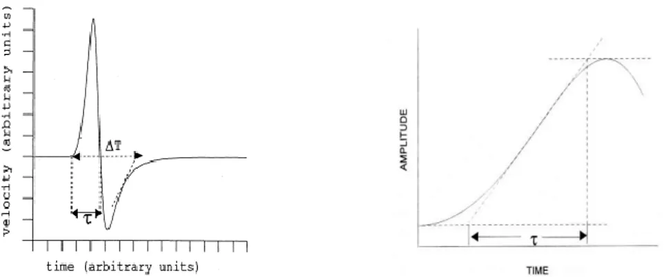
Different definitions of rise time have been proposed in the literature. Gladwin and Stacey (1974), for example, defined it as the maximum amplitude divided by the maximum slope on the seismogram. Zollo and de Lorenzo (2001), on the other side, define the rise time in a velocity signal as the interval between the arrival time and the first zero crossing time (fig.1.3).
Irrespective of definition, the rise time value is expected to increase with the distance travelled by the wave; in particular, Kjartansson demonstrated that, when considering the propagation of a pulse of a Dirac’s delta throughout an anelastic medium characterized by an exactly constant Q, the relation between and t* is completely
linear:
* 0C Qt
15
In the above equation, is the rise time at the source, whereas the slope C(Q), is a function of Q. About this term, a lot of studies have been carried out in the past: Gladwin and Stacey (1974) have experimentally found a constant value of C to be equal to 0.5.
Blair and Spathis, (1982), on the other hand, for Q>30 have found different C values depending on the type of records: in particular values of 0.485, 0.298 and 0.217 for displacement, velocity and acceleration records have been found, respectively; de Lorenzo (1998), furthermore, in accordance with Blair and Spathis (1998) conclusions, suggested the C dependency on the shape of the source time function. In particular de Lorenzo (1998) demonstrated that the linearity between and t* remains only at a corner frequency of the source greater than 10 Hz. In all other case, the dependence of C(Q) on source spectrum implies that the classical rise time method can lead to biased estimates of attenuation when applied to earthquake data.
The greater advantage of this method is that, with respect to spectral techniques, it is not affected by subjective windowing criteria; furthermore, because the method is principally based on the observation of the first pulse broadening in the signal, it allows to discard the secondary contributions coming from heterogeneities inside the propagation medium.
On the other hand, “the greatest limit of the technique is that it completely neglects the directivity effect of the seismic radiation generated by a finite dimensional seismic source” (cfr. Tselentis, 2011). However, Zollo and de Lorenzo (2001) proposed in this case a method to deal with the nonlinearity between the rise time and the travel time and to account for directivity of the seismic source. In the case of an active seismic source, obviously, the directivity effect can be neglected. Furthermore, spectral ratio method can be susceptible to bias from noise, so that only high S/N ratio traces can be considered in the analyses.
By means of this method, an estimation of Q in the approximation of an homogeneous medium can be retrieved.
To this purpose, the relation (1.33) has to be considered; in particular, the rise time measurements ( on seismic signals contain the undesired source term, which is totally independent of the anelastic attenuation.
16
For this reason, for each event the different source contribution has to be removed from rise time measurements.
This can be achieved by fitting, for any individual event, the distribution of measured rise times as a function of the travel time T: the point where the best fit line intersects with the rise-time axes is that is the rise time at the source (fig. 1.4 c). This retrieved
value has to be subtracted from the measured rise times, obtaining the so called “reduced rise time” (Tselentis et al., 2010).
In this way, a common distribution of rise time measurements as a function of travel time is obtained, including all the analysed events (fig. 1.4 b). By fitting the distribution and by assuming the term C(Q) as a constant, the slope of the best fit line will directly give a first estimation of the mean value of the quality factor in the propagation medium.
This method has been widely used in literature for attenuation tomography works (e.g. Zucca et al., 1994; de Lorenzo et al., 2001; Tselentis et al., 2010).
Figure 1.3. Left: Rise time as defined and measured by Zollo and de Lorenzo (2001) in velocity
seismograms (after Zollo and de Lorenzo, 2001) . Right: Rise time definition by Gladwin and Stacey (1974) (after de Lorenzo, 1998).
Figure 1.4. Left: Increasing rise with hypocenter distance. Right: Plot of measured rise times for a
17
1.5.2 The Spectral ratio methodThe spectral ratio method was originally proposed and formulated by Teng in the 1968; Teng (1968) studied the variations of the quality factor in the deeper part of the mantle analysing earthquake data.
An observed P wave amplitude spectrum can be expressed as the product of a source function S
f,,
with a number of transfer function each for an appropriate portion of the transmitting medium.
*
exp , , C f Gt I f ft f S f A , (1.34)where the site effects are accounted by C(f), the path geometrical spreading is represented by G(t), whereas the instrumental response by I(f).
The anelastic attenuation effect is represented by the exponential term exp
ft*
. Before facing in detail the principles of the method, two basic assumptions necessary for its application when considering earthquake sources must be underlined:1) the normalized source spectrum is not a function of spatial coordinates;
2) the attenuation function can be expressed in terms of a frequency-independent Q over the frequency band by the exponential quantity exp
ft*
.According to the first assumption, the source term S
f,,
can be separated in two terms, a spatial and a temporal part, giving the expression
f,,
St
f Ss ,S . (1.35).
Among all the terms appearing in the (1.34), only the exponential quantity has to be considered in attenuation studies.
The spectral ratio method allows very easily to overcome the common problem of ignoring and removing the contributions of factors different from the one we are interested to, as the source effect and the instrumental response. This is achieved by the computation of the ratio of the amplitude spectra recorded by two receivers located at different distances, x2 and x1, from the source. (fig. 1.5).
The station respect to which the spectral ratio is computed is the so called reference
station. Its choice can be arbitrary, but sometimes closest station to the source can be
chosen as reference receiver: it would allow to neglect the attenuation contribution and to consider the respective signal as an approximate representation of the source signal.
18
Fig. 1.5: Simple scheme of source-stations configuration for the application of spectral ratio method.
Then, taking the spectral ratio with respect to the reference receiver, station 1, at the distance x1,:
S
f S C f x
G t x
I f
t f
f t f I x t G x f C S f S x f A x f A s t s t j i * 1 1 1 1 * 2 2 2 2 1 2 exp , , , exp , , , , , . (1.36)It is evident that for a common shot gather with an explosive source and with stations using the same type of instrument ( that is the same response curve), quantities St(f) and
I(f) for both spectral signals cancel out.
By making the assumption that site responses at the two different receivers are equal,
C(f,x
1) and C(f,x2 ) in (1.36) approximately cancel out, and the equation will take the
form
G
x S
t f
f t S x G x f A x f A s s * 1 1 1 * 2 2 2 1 2 exp , exp , , , . (1.37)Taking the logarithm of the equation (1.37), we can deduce the expression
1*
* 2 1 1 2 2 1 2 , , ln , , ln f t t S x G S x G x f A x f A s s , (1.38)with a linear slope c equal to f(t*2 – t*1) (Matheney and Nowack, 1995). It is retrieved
by fitting in the sense of least-squares method the logarithm of the spectral amplitude ratio. The term (t*2 – t*1) is called differential attenuation term and contains the whole
information concerning the difference of wave attenuation along two different rays. i
19
1.5.3 The spectral decay method
The spectral decay method theory is based on the description of the displacement spectra already presented in equation (1.34).
In particular, this measurement technique is based also on the a priori knowledge of the source function. Source theories for earthquakes predict a spectral shape similar to that given by the theories for explosions: a constant long period level, ( proportional to the seismic moment M0), followed by a decay above the corner frequency fc. Generally
the decay is described by an exponential function f -n, where n is a value between 2 and 3 and is defined as high frequency spectral fall-off parameter (Cormier, 1982). Mathematically, the temporal part of the source spectrum is defined as
n c t f f f S 1 ) ( 0 . (1.37)
One of the greatest problems in estimating anelastic attenuation properties from earthquake spectra is the existing trade-off between Q measurements and source parameters (in particular the corner frequency and the high frequency spectral fall off). In fact, Q affects the spectral shape at frequencies smaller than the corner frequency, whereas at frequencies higher than the corner frequency both n and Q control the spectrum (Zollo et al., 2014).
Figure 1.6 Example of the application of spectral ratio technique on synthetic signals
produced in an homogeneous model, both in elastic and anelastic properties.
a) Amplitude spectra recorded at two different distances from a point source located at a
depth of 3 km; dashed line: farther receiver; solid line: reference station. b) Spectral ratio computed between the two amplitude spectra represented in figure a). The computed spectral ratio is perfectly linear, because of absence of noise in synthetic signals and homogeneous elastic and anelastic properties.
20
It means that at frequencies higher than the corner frequency the decay will be proportional to f -n times the exponential factor exp
t*f
describing the anelastic attenuation.However, for low magnitude earthquakes (ML 1) the corner frequency is shifted
toward highest frequency values: it means that, in presence of anelastic attenuation, low frequencies should show a spectral decay proportional to anelastic properties of the medium (together with the contribution of site effect and instrumental response).
By removing these undesired contribution (actually, regarding the site effect, this procedure is not so trivial (cfr. de Lorenzo et al., 2010)), and computing the natural logarithm of the amplitude spectrum we have
f Q t k f Aij ln ) ( ln , (1.38)
where the indexes i and j represent the source and the receiver indexes, respectively. From (1.38), the slope of the best fit line of the logarithm of the amplitude spectrum in an established frequency range is proportional to the quantity t* (Wittlinger et al., 1983).
Figure 1.7 An example of the application of spectral decay
method in order to retrieve t* measurements. The slope of the linear trend gives a rough idea of the attenuation influence (after Wittlinger et al, 1983).
A similar approach can be followed in the case of a point explosive source, whose spectrum can be assimilated to the Dirac function’s one.
On the other hand, for earthquakes of magnitude greater than 1, the corner frequency is shifted toward lower frequencies. It means that it is not possible to retrieve so easily the
21
t* parameter without taking into account the existing trade-off between Q and source parameters. Different techniques have been developed in the past year; they, in particular, consist in iterative procedures in which, at different steps, different inversion parameters (fc, t*) are retrieved (Edwards et al., 2008; Zollo et al., 2014).
22
CHAPTER 2
Data analysis: validation of spectral ratio
method through synthetic tests
.
2.1 Introduction
As described in the previous chapter, different techniques for estimating anelastic properties have been developed and used in literature in order to obtain attenuation images of the Earth.
In my PhD thesis, the spectral ratio method has been used and its applicability to our purposes has been tested.
This method has been chosen because source contribution and the instrumental response may be removed from the amplitude spectra of the signal. In spite of this advantage, spectral ratio method has met with lot of criticisms because of its instability.
The first aspect which causes the method to be instable is common to all spectral methods: the necessity to isolate a proper time window.
In fact, in order to retrieve informations on the anelastic effect on an established seismic phase (P or S wave), the respective portion of signal has to be isolated from the seismic trace.
Actually, the risk to include other phases than the one we are interested to must be avoided. Sometimes, these complications may be due to the presence of multiple arrivals after the phase we are looking at. As the seismic waves spread away from the source, the different component of the wavefields interact with crustal structure in a variety of ways. These interactions may lead to quite complex behavior, causing elongated wavetrains and complexities in the waveforms. These signal features can be originated by different factors: 1) the scattering produced by heterogeneities in the propagation medium; 2) the thin layering generating multiple reflections and converted phases at shallow depths; 3) a strong velocity gradient. The selection of the proper time window is, therefore, an important issue. In fact, a short time window generally allows
23
to remove and to neglect all the secondary arrivals. Clearly, the selected time window has to start from the arrival time of the phase whose spectrum has to be computed. On the other hand, a too short time window determines a low resolution at low frequencies and a low spectral resolution. This is reflected in few points over which to fit the spectral ratio. In these conditions it has been seen that the resulting spectral ratio becomes highly variable (Goldberg et al., 1984; Sams and Goldberg, 1990), having a trend far from a linear trend. Sams and Goldberg (1990), furthermore, confirmed the results of Ingram et al., (1985): they found that errors introduced by windowing are minimized when the window duration is long. White (1992), furthermore, showed that the variance in differential measurements by spectral ratios method is inversely proportional to the time window length used in the spectral amplitude computation. Obviously, the best compromise between duration of the time window and spectral resolution must be found. Actually, too long time windows more likely will contain seismic phases different from the interest one.
Matheney and Nowack (1995) faced the problem of the choice of a proper time window by selecting a variable window length. In particular, they chose a duration equal to three times the first arrival time to envelope peak. This selection criterion was tested both on spectral ratio method and on instantaneous frequency matching method. It was demonstrated that this procedure is able to effectively isolate the first arrival without selecting a too short time window which makes unstable the spectral ratio.
An intrinsic problem linked to the windowing has to be considered, too: the selection of a portion of the signal is obtained by the product of a box function for the seismic trace. In the frequency domain, this operation corresponds to the convolution of the seismic signal FFT with a sinc function. The effects of this mathematical computation introduces nodes and peaks in the windowed spectra. However, the main concept is that by computing the ratio, the effects produced by the convolution with a sinc function at both the spectra do not cancel out. This aspect, unavoidably, introduces further complications and irregularities in the resulting spectral ratio which may only be damped by applying a smoothing procedure to spectra.
Another element renders difficult Q measurements through spectral ratio technique. Actually, in spectral ratio method attenuation measurements are conducted using seismic amplitudes: for this reason noise disturbances have to be taken into account in the analysis of the signal.
24
Furthermore, seismic amplitudes are strongly affected by the Earth’s complex velocity structures and by other factors: among them, the free surface effects on the wave field may be mentioned. Generally, these elements are not taken into account in the modelization of the amplitude spectrum. Actually, the path effect is usually simply described as the product of the geometrical spreading with the attenuation factor. The geometrical divergence is commonly described in the very simple exponential formulation r . In the previous formula the distance is expressed by r and the term is a factor depending on the wave type (andfor surface and body waves, respectively). Naturally, in complex velocity structures, in particular in the near surface, this description is a rather simple approximation to use in order to describe amplitude variations of the seismic signals.
Concerning this, Sams and Goldberg (1990), in a borehole data study, concluded that a such simple geometrical divergence model was one of the causes of their bad Q estimations. In particular they obtained more reliable attenuation measurement by numerically estimating the divergence term and deconvolving it from experimental amplitude spectra. Practically, it means to compute through numerical simulations the elastic Green’s function in a medium without attenuation. To this purpose, elastic properties of the medium, that is velocity and density model, have to be known. Actually, the Green’s function term will include effects of complex interactions, energy partitioning among various wave types along layer boundaries, as well as focusing/defocusing effects. All these phenomena may generate inhomogeneous waves or leaky modes and are completely neglected by the geometrical spreading factor: this aspect, therefore, can affect the resulting Q measurements.
Then, the greater is the knowledge of the heterogeneity of the medium, the more accurate will be the retrieved elastic Green’s function with respect to the real unknown medium structure. As a consequence, Q measurements will be closer to real attenuation values.
Based on all these considerations, a preliminary phase of study has been carried out. It was aimed to test the validity of the spectral ratio method and the reliability of the consequent dt* measurements.
25
Synthetic tests have been performed in order to know the sensitivity of the spectral ratio method to different factors, that is: 1) velocity model; 2) selected signal time window; 3) frequency range over which the spectral ratios are computed and fitted.
Although, theoretically, through spectral ratio the source contribution is completely deleted from the spectrum, also the sensitivity of the method to two different types of sources has been investigated.
Finally, a method to take into account the complexities of the medium and to remove their effects from seismic signals has been tested on synthetic signals.
This methodological study has been aimed at the elaboration of a procedure for the dt* computation on real data.
2.2 Synthethic tests
Synthetic tests have been performed on synthetic seismograms, which in turn have been obtained computing the Green’s function by means of AXITRA (Coutant, 1989). It is a numerical code which implements the discrete wave-number Bouchon's (1981) theory in conjunction with reflectivity method (Kennet, 1983). The computation of Green’s functions takes as input a 1D layered model of velocity, density and attenuation, as well as earthquake/shot position, source origin time and stations locations.
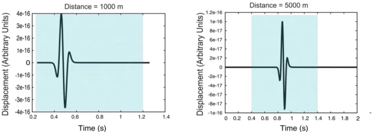
In detail, ten synthetic seismograms have been generated at progressively increasing distances from the 300 m shallow explosive source. In particular the receivers are located at the free-surface at epicentral distances from 1 km to 10 km, with an inter-receiver distance of 1 km (fig. 2.1). The source depth of 300 m has been chosen in order to simulate a surface source: actually, the numerical code does not allow to position both receivers and source on the free surface. Furthermore, an initial test using a 3 km depth source has been performed. Synthetic signals are characterized by a time sampling of 0.004 s. It corresponds to a Nyquist Frequency equal to 125 Hz and a maximum anti-aliasing frequency equal to 62.5 Hz.
The computed Green’s functions in most tests have been convolved with a 0.2 s duration Ricker source; the unique closest station to the source (epicentral distance equal to 1 km) has been used as reference receiver. In other tests, Green’s elastic function have been convolved with a 0.2 triangular source, too. All the following tests have been conducted only on P waves.
26
Figure 2.1. Source-receivers configuration used in synthetic tests. The red point represents the source,
the blue triangles the stations. The receivers are located at the free surface, at epicentral distances from 1 km to 10 km, with an inter-receiver distance of 1 km. The source is located at a depth of 300 m.
In order to test on synthetic signals the reliability of dt* measurements, these have been compared with theoretical dt* values. Except for the trivial example of an homogeneous model both in elastic and in anelastic properties, the theoretical dt* have been computed through the direct part of the tomographic inversion code TOMO_QDT. It is the adapted version to the case of the attenuation of the tomographic inversion code TOMO_TV.
A complete description of the numerical code will be given in the fourth chapter of this thesis, in which also the details about the modification that we brought to the code will be provided. In this paragraph, instead, the way in which the theoretical dt* are computed is briefly described.
The forward problem of dt* computation has been faced through the computation of absolute t*. First, the propagation medium is modelled by means of a tridimensional inversion grid of nodes, at whose correspondence a quality factor (QP) and a velocity
value (VP) is assigned. Actually, only 1D velocity and attenuation models have been
considered, so that at each depth the grid nodes have all the same value of quality factor and velocity.
Since t* values depend on the ray paths, the ray tracing has been previously performed. Ray paths depend only on velocity model and they have been retrieved by solving the Eikonal equation with a finite difference algorithm (Podvin and Lecomte, 1991). For this computation, a grid finer than the inversion grid is required; the velocity values of each node of this finer grid are obtained through a trilinear interpolation of the tomographic inversion grid. Podvin and Lecomte (1991) algorithm allows for each source-station couple to obtain a first estimation of travel time at each node of the fine
27
grid. Therefore, it is possible to obtain the ray path through a back ray tracing by following the gradient of the estimated travel times.
After the computation of ray paths, a refined estimation of t* values is retrieved through the integration of along the traced rays. The quantity represents the reciprocal number of Q.
After theoretical t* for every source-receiver couple have been obtained, the differential values, dt*, are obtained by computing the difference between the corresponding t* values.
2.2.1 Sensitivity of the method to V(z) models
The validity of the spectral ratio method and of dt* measurements has been tested in different models with V(z) depending on depth. All the performed synthetic tests are characterized by 3 p S V V and =2700 kg/m3.
V(z)=cost and deep source
In this test a homogeneous velocity (Vp=6.5 km/s) and attenuation model (Q=100) have been implemented.
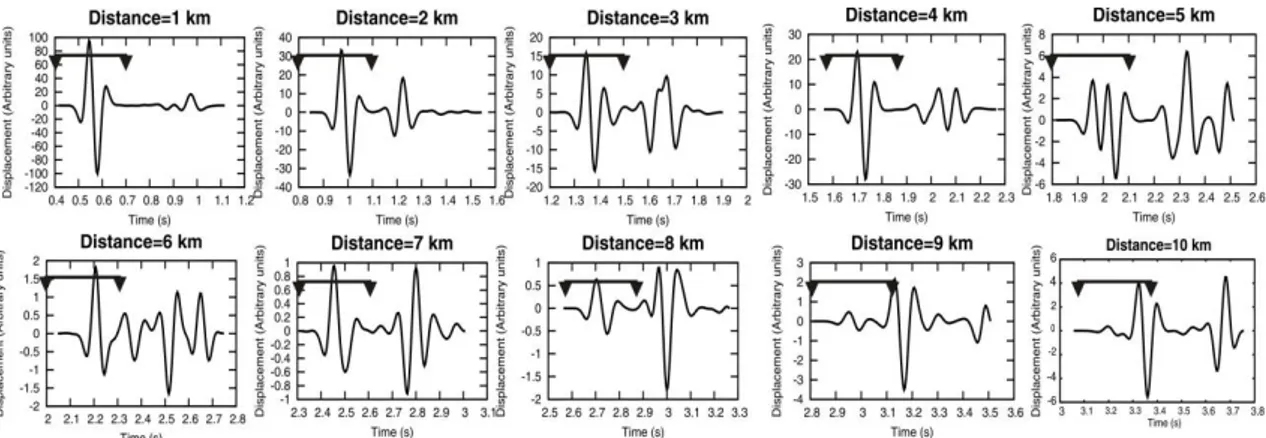
Two different signals for receiver 1 and receiver 5 are shown in the figure 2.2 as an example; their spectra and the relative spectral ratio are also shown in the figure 2.3. In figure 2.3 the dt* measurements as a function of R are shown overlapped to theoretical dt* values, too. The quantity R, here, is the difference of the distances travelled by the two signals recorded at two different receivers; obviously, this quantity depends on the ray paths. It means that, with the same source-receivers configuration but changing the velocity models, R quantities will be different.
A 1 s time window around the first arrival has been chosen; we are allowed to use such a large time window because no secondary arrivals are present in seismograms. Before computing the fast Fourier transform of the synthetic signals, zeros were added to 28 points. In that way a time window of 1.020 s, corresponding to a minimum frequency in the amplitude spectra of 0.98 Hz, has been obtained. Then, also the sampling of lower frequencies is guaranteed.
28
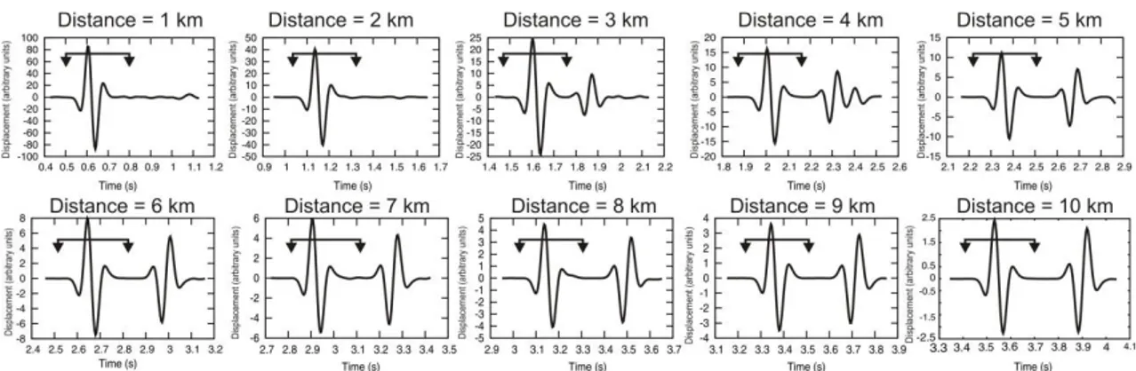
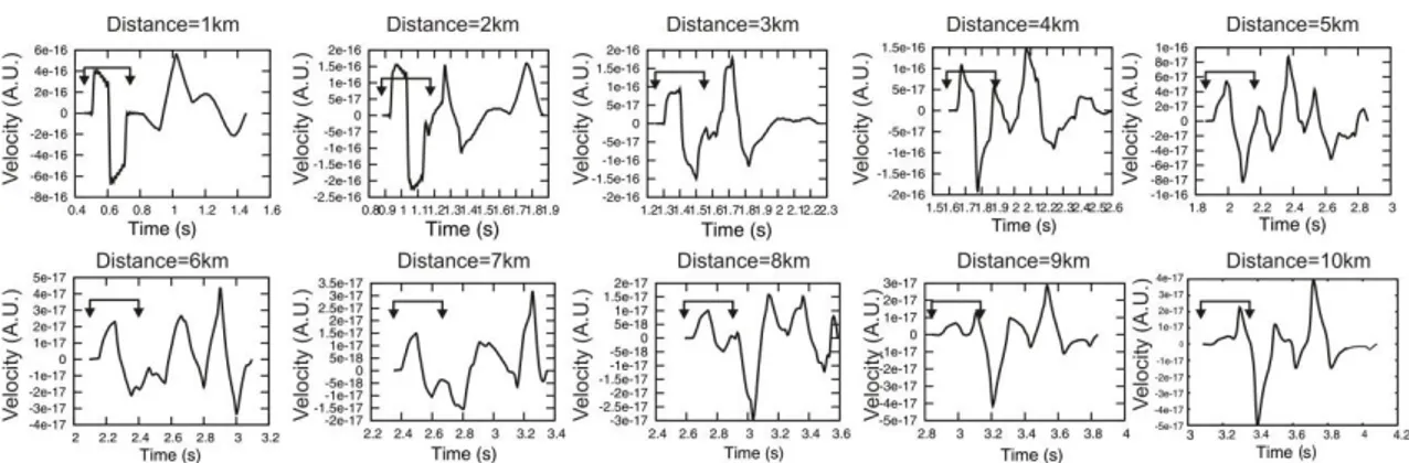
Figure 2.2. Synthetic displacement seismograms at two different receivers. They are located at 1 km and
5 km epicentral distances, respectively. The cyan lightened area represents the portion of the seismogram that has been used to compute the amplitude spectra.
Figure 2.3. a) Amplitude spectra of the signal recorded by the reference station (solid line) and by the
station 5 km far from the source (dashed line). b) Spectral ratio computed between the two amplitude spectra represented in figure a). c) Comparison between theoretical (red points) and measured dt*(black triangles). There is a perfect agreement between measured and theoretical dt*. Furthermore, by fitting the dt* distribution as a function of R in the sense of least-squares, a Q=100.15 is retrieved.
Based on results shown in figure 2.3, we can conclude that in optimal conditions, that are deep source and homogeneous model, spectral ratio method provides reliable dt* estimations.
Shallow source and V(z) velocity models
.
The propagation of a wave field produced by a source (both an earthquake source and an explosive one) is greatly affected by the elastic properties of the medium in which waves travel.
A deep attention has been focused in this section on the velocity model. Actually it not only influences the arrival time of the waves at different receivers, but most of all it contributes to the generation of phases other than direct ones.
29
It is clear that in real conditions it could be very difficult to isolate phases different from the direct one; this depends on the possible overlapping of the phases and on a contamination of the signal to which we are interested.
The following synthetic tests have the aim to show the effects of velocity model on time domain signals and on their spectra, looking at the way they are reflected into dt* measurements.
In particular, at first we have investigated the applicability of spectral ratio method in a gradient velocity model. After that, in order to give an answer about the applicability of the method in a real area, velocity models describing the elastic properties of Campi Flegrei area have been considered.
In detail, a continuous representation of Judenherc and Zollo 1D velocity model (2004) (JZ hereafter), an its smoother representation and the average 1D model obtained from 3D Campi Flegrei model (Battaglia et al., 2008) have been used.
An attenuation halfspace (Q=200) has been considered.
In these tests the source is shallower than the previous one (it is located at a depth of 300 m). The receivers configuration is the same of the previous one (fig. 2.1).
Gradient velocity model-MODEL 1
Also in this case, synthetic seismograms have been obtained convolving Green’s functions computed by AXITRA with a 0.2 s duration Ricker source.
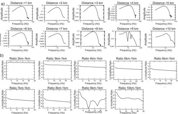
From figure 2.5 it is clear that also with a simple gradient velocity model a shallow source produces arrivals different from the P direct ones. They are due to free surface effects and generation of inhomogeneous waves. From an analytical point of view, it means that by using a very large time window, secondary arrivals will be included.
30
For this reason a 0.3 s time window has been chosen, starting from 0.05 s before the manually picked P first arrival time. Furthermore, zeros were added to total 27 points. A cosine taper window of 10% fraction of tapering has been also applied to the cut signal in order to reduce the contribution of fictitious high frequencies in the amplitude spectra.
By considering the sampling time of the signal of 0.004 s, and the anti-aliasing corrections, the maximum frequency is 62.5 Hz. Since a zero padding has been done in order to compute fast Fourier transform of the signal, df is not equal to 3.33 Hz. Actually it is equal to 1.95 Hz. Finally, amplitude spectra have been smoothed with a moving 3 points averaging window.
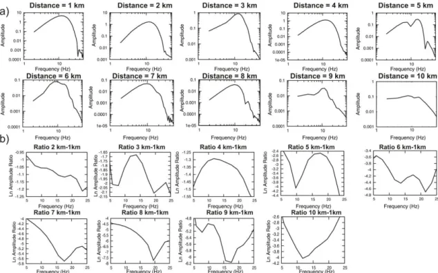
The retrieved spectral ratios and measured dt* are represented respectively by figure 2.6b and figure 2.7. The dt* have been estimated by fitting the spectral ratio in the least-squares sense in the frequency range 5-25 Hz. The upper limit of the frequency range over which to fit the spectral ratio has been chosen looking directly at the individual spectra. It has been observed that for frequencies greater than 25-30 Hz the spectral amplitude is not meaningful.
Taking into account the df and the selected frequency range, then the spectral ratio has been fitted on a number of points equal to 10.
In particular it is possible to observe a very good fit between theoretical and measured dt*, except for the 9/1 and 10/1 spectral ratios which correspond to Q estimations of 186 and 270 respectively (the theoretical QP value is equal to 200).
Figure 2.5 Synthetic displacement seismograms generated by a shallow Ricker source and recorded at
all receivers in a gradient velocity model. The traces have been cut in a 0.7 s time window only for this representation. The signal processing has been done, instead, on a 0.3 s signal time window (represented by the bar in each seismogram panel). It starts 0.05 s before the manually picked P first arrival.
31
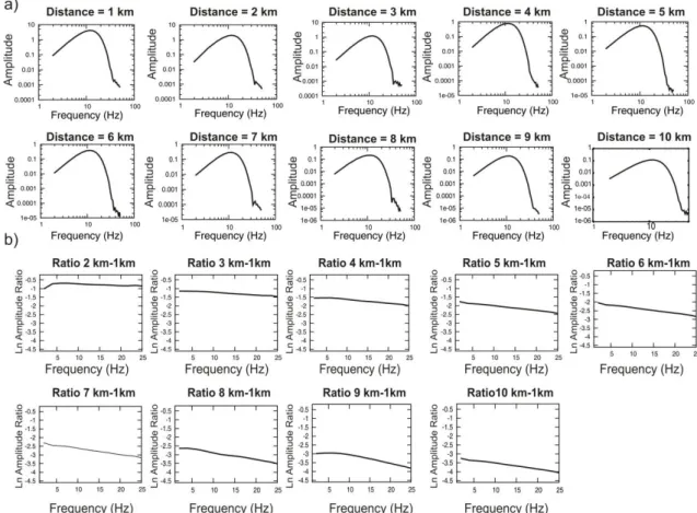
Figure 2.6 a) Amplitude spectra of the synthetic signals recorded at the ten receivers. The amplitude
spectra are very smooth and do not show any peak or spectral holes. b) Retrieved spectral ratios represented in the range 1-25 Hz; the higher frequencies are not represented because of the numerical noise visible directly in the amplitude spectra. A great linearity in the spectral ratios is observable: it is reflected in very small uncertainties in dt* estimations.
Figure 2.7 Comparison between theoretical (red points) and measured dt* (black triangles): the
agreement between them is very good, except for the ratio 9/1 and 10/1, for which the differences between estimated Q and real one correspond respectively to -14 and 76.
32
JZ (2004) 1D velocity model-MODEL 2The JZ 1D velocity model (2004) has been obtained from a tomographic study starting from the analysis of SERAPIS data set and part of Tomo-Ves 97 experiment data. It is a layered model, each layer having a thickness of 250 m.
Because, in the reality, Earth elastic properties gradually change, a continuous representation of JZ 1D velocity model has been used. It has been obtained linearly interpolating JZ 1D model. Then, by stacking homogenous plane layers having a thickness of 25 m, the velocity model has been constructed. After all, the Volterra theorem (see Gilbert and Backus, 1966) states that “wave system propagating in a medium with continuous spatial variations of density and wave speeds can be studied by solving for the waves in a discrete medium composed of many homogeneous parts” (cfr Aki and Richards, 1980).
Furthermore, the original JZ 1D model shows very strong velocity discontinuities among each layer; since Green’s function are computed through reflectivity method, such velocity jumps are reflected in a great complexity of waveforms. On the other hand, the constructed continuous medium above described allows to obtain simpler wave forms, which can be more easily interpreted.
Simply looking at the velocity model, a strong velocity gradient at about 1.5 km is clearly visible. Furthermore, at greater depths (2 km and 2.5 km) two little velocity inversions are present.
Figure 2.8 Continuous representation of JZ 1D velocity model.
Figure 2.9 shows that in addition to the presence of distinct secondary arrivals, P first arrivals are very often contaminated by interferences linked to the complexity of the