3D CNN for classification of brain MRI

(1)

POLITECNICO DI MILANO

School of Industrial and Information Engineering Master of Science in Biomedical Engineering

3D CNN for classification of brain MRI

Supervisor: Pietro Cerveri

Thesis of: Marco Passa Student ID: 899075

(2)

2

Acknowledgements

I would like to thank Prof Cerveri, without his collaboration would not possible make this partnership.

Then I would like to thank Maria Lusia Mandelli and Yann Cobigo for the help with the project.

Finally I would to thanks my family (Carla, Sara, Miria, Luca, Marco, Sesa, Elena, Cynthia e Francesca) for the inspiration and support they have always transmitted to me.

(3)

3

Abstract

Currently there is not established automatic methodology for identifying patients with language deficits with an AD vs. no-AD pathology. Neurologists presently diagnose the patient population under a manual process that is time-consuming and expensive. Convolutional neural network has been widely used for the image processing in the medical field in the last years for tasks that were not possible to realize with the classical software. Research has shown that the CNN can be used in the medical field for various tasks like image denoising, segmentation and classification. In this study we build two CNN model: one for 3-D MRI brain denoising and one for 3-dimensional MRI brain classification to distinguish patients with language deficits with AD pathology versus no-AD pathology.

We want to establish if it’s possible use this method also with a very small data set, made by 45 brain MRI patients for each group and 45 control subjects. In this context, a good classifier is defined as a model that can classify at least with the 70% of accuracy on data on which it is not trained on.

Based on a review of the literature, there are various architecture and methods to implement efficient CNN model also with small dataset. Regarding the architecture we used the 3-dimensional version of the convolutional layer and of the other visual processing layer that is a new

(4)

4

introduction in the field and show very good result on 3-dimensional images. The result with the best model created did not reach the 70% of accuracy instead the 62%. The all project has not to be consider a fail because the goal of the project was very difficult to reach for the small number of data, but still we get closer and during our experiments we understood which are the best CNN architectures for image processing of 3-dimensional images.

(5)

5

List of figures

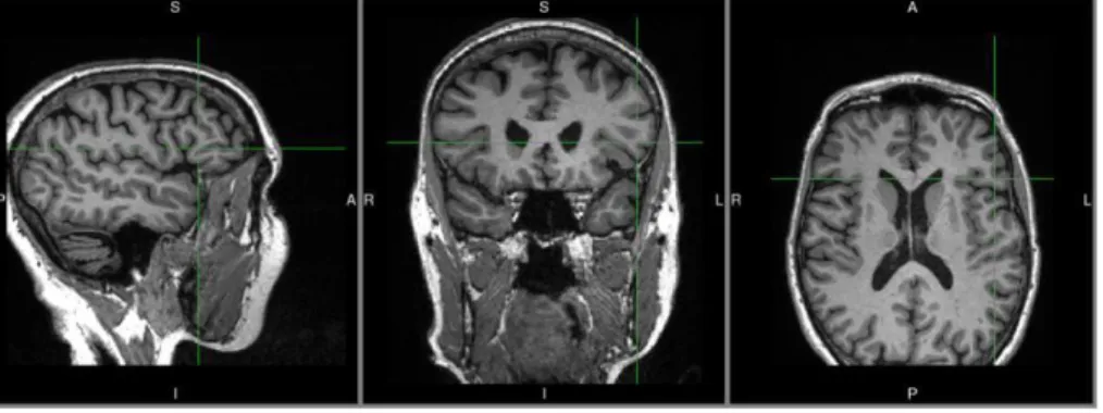
Figure 1: Example of PPA patient diagnosed as nfvPPA MRI ...16

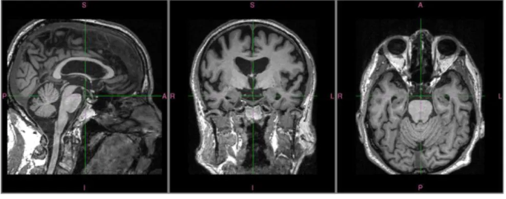
Figure 2: Example of PPA patient diagnosed as lvPPA MRI ...17

Figure 3: Example of healthy subject MRI ...17

Figure 4: Example of MRI without pre-processing ...23

Figure 5: Example of MRI after cropping ...24

Figure 6: Example of MRI after cropping and rotation ...25

Figure 7: Graphic representation of 3D-convolution layer ...28

Figure 8: Graphic representation of the differences between convolution and deconvolution layers ...29

Figure 9: Graphic representation of Max pooling layer1 ...30

Figure 10: Graphic representation of Fully connected layer ...31

Figure 11: Graphic representation of ReLU function ...32

Figure 12: Graphic representation of SoftMax function ...33

Figure 13: Example of MRI used as input ...37

Figure 14: Example of MRI used as target ...37

Figure 15: Scheme of the model 1 of denoising case ...39

Figure 20: Scheme of the model 1 of classification case ...46

(9)

9

Figure 25: Loss function during the training model 1 ...53

Figure 26: Image generated by the network model 1 ...54

Figure 27: Histogram representing the error of the input(blue) and the output(green) respect the target model 1 ...54

Figure 41: Accuracy during the training model 1 ...64

(10)

10

Figure 50: Accuracy on the test set every 2000 iterations model 5 ...72

Figure 51: Table of result of classification accuracy ...73

Figure 52: Main Processing Unit ...79

Figure 53: Example of multilayer feed-forward network implementing two hidden layers ...81

(11)

11

1 Introduction

The majority of brain diseases diagnosis are still based on the evaluation of a doctor and still are not presents solid software that can automatize the process. We want to implement a software that is able to recognize and classify two different cohort of patient with primary progressive aphasia the non-fluent (nfvPPA) and the logopedic variant (lvPPA) from the 3-dimension brain MRI image of the subject. To do this we chose to use a machine learning technique, artificial neural networks. In the present years these methods are been used with success in a lot of areas, also in the medical field area. In specific we are going to implement a convolutional neural network, that is a specific ANN specialized for image processing, that process the data directly in 3-dimension, that result from the state of art more efficient on 3-dimension images. The most common problem of the implementation of ANN in the medical field is the missing of big dataset. To solve this problem, we are going to experiment different network and different pre-processing technique for data augmentation till reach the best model for the task.

1.1 Clinical context

Primary Progressive Aphasia (PPA) is a clinically and pathologically heterogeneous neurological condition characterized by progressive and selective language and speech impairment. International guidelines were able to establish a classification of the main variants [1]. The guidelines use

(12)

12

all the knowledge accumulated since the last 20 years based on language dysfunction, brain atrophy and underlying pathology. In particular, two of these variants are very difficult to distinguish: the non-fluent (nfvPPA) and the logopedic variant (lvPPA). The nfvPPA is characterized by grammatical errors in sentence production, along with motor speech-based effortful and halting speech production and phonetic-motoric errors of phoneme distortions [2], damaged in the left inferior frontal gyrus, premotor cortex, supplementary motor cortex and temporal brain regions, and it is usually caused by fronto-temporal lobar degeneration (FTLD), mainly tau [3] (including Pick disease, corticobasal degeneration, progressive supranuclear palsy). The lvPPA is characterized by short-term memory deficits for sentence repetition, phonological errors of speech sound substitution, damaged in the left parietal and temporal brain regions, and it is usually caused Alzheimer disease pathology (amyloid-Beta plaque deposition) [4] [5] [6].

Up to now, in-vivo amyloid brain imaging is available through the fluorinated amyloid positron emission tomography (PET). Instead, no in-vivo imaging techniques are available to detect tau inclusions alike for FTLD.

Only pathological reports represent the gold standard to define the underlying pathology these disorders. Moreover, PET scanning is an expensive technique and often not available in routine practice. Therefore, in the clinical routine, these patients are required to go through an extensive speech and language battery requiring an huge effort from an equip of specialized professional (neurologist, behavioral neurologist, speech

(13)

13

language pathologist, neuroradiologist). At the Memory and Aging Center of the University California San Francisco (UCSF), it is available the best characterized cohort of Primary Progressive Aphasia with 20 years of specific knowledge of this disease. By taking advantage of this cohort, an automated classifier that learns from this cohort and predicts the underlying pathology (AD or no AD), it would be of extremely impact in the clinical contest. The main reason why it is important to predict the underlying pathology is that therapeutic interventions target specific aggregates characteristic of the pathology underlying the disease.

1.2 Artificial Neural Network in medicine

Artificial Neural Networks (ANN) offer a powerful set of tools to analyze clinical data over a vast range of medical applications.

The most common applications are prediction, differential diagnostic and segmentation task. For example, in a classification problem, we want to predict in which class a patient would fit after the neural network has been trained on specific clinical features.

Medical classification can be problematic as it is often based on human medical judgment. The use of neural network (ANN) in the medical fields have exploded in the past few years. Like in the other fields principally because the increased number of data and the dimension of data and for the introduction of GPU that make possible analyze those big data [7].

The most common problem in the medical field though are the heterogeneity of the data and thelack of copious data in respect to the other

(14)

14

fields [8]. The first problem can be solved by choosing a heterogenous training set and for the second there is some data augmentation techniques like rotating the images to generate new data [9].

1.3 Goals of the thesis

The cases of this project are 2: • Denoising;

• Differential diagnostic classification.

The first case consists in creating a machine learning model that is able to take a brain scan MRI and produce the same 3-dimensional image as output but with a reduced quantity of noise. The second case is the creation of a machine learning based model that can classify the condition of a patient in 3 class:

• Pib positive; • Pib negative; • Control.

(15)

15

1.4 Result

The result obtained shows that with the small data set of images that was present at this point in the UCSF database is not enough to use machine learning technique. The model is able to recognize the difference between the 3 different class, but the number of data is not enough to generalize the model to the hole population and to classify with good accuracy also data non present in the training set.

For having good result in term of classification the number of data has to grow at least of a factor of 10, before this quantity of data will be accessible the machine learning technique are not efficient.

(16)

16

2 State of art

In this chapter I am going to introduce first how is form now diagnosed and make the classification that we want to automatize and then introduce the other project that has good result in biomedical image processing generally using artificial neural network technique.

2.1 Clinical context

From the clinical point of view, the diagnosis of Alzheimer disease and his form is diagnosed manually by the doctor. The doctor bases his diagnosis on principally the MRI images of the brain.

For this study, we identify 2 cohorts of patients that were diagnosed as nfvPPA or lvPPA by the specialized equip, had a 3D T1 structural brain image, and underwent to a PET scans or had a pathological report [10].

• Cohort 1: 45 PPA patients diagnosed as nfvPPA, with a structural

T1, a negative amyloid PET scan or FTLD as pathology;

(17)

17

Cohort 2: 45 PPA patients diagnosed as lvPPA, with a structural T1

positive amyloid PET scan or AD pathology;

Figure 2: Example of PPA patient diagnosed as lvPPA MRI

Cohort 3: 45 Healthy subjects matched to the patients for age and

gender, with a structural T1, and negative for AV-45 amyloid-PET.

(18)

18

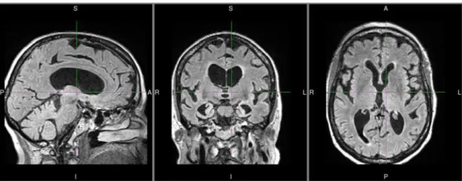
The cohort 1, nfvPPA patients, are identified by a degeneration of grey matter in the right temporal lobe (see fig. 1) instead the cohort 2, lvPPA patients, are identified by degeneration of gray matter in the right parietal lobe (see fig. 2). The control subjects, cohort 3, do not present gray matter degeneration in specific region of the brain (see fig. 3) [11][12].

2.2 Methods

for

images

processing

and

classification

The artificial neural networks are becoming very used in the medical image field. The main tasks for which they ANNs used are: image denoising, image segmentation, image classification.

This machine learning technique is better respect other ones like super vector machine because they do not need long preprocessing technique and has better performance on computational efficiency and accuracy of the result [13].

The bigger disadvantage of the ANNs respect the other machine learning techniques is that they need a bigger number of data to generate a model that can works correctly also with new data non present in the data set [14].

In this project we are going to use 3D visual layers instead of the classical 2D visual layers.

The better performance of the 3D visual layers respect the form in 2D is already proved on task like:

(19)

19

• 3D-MRI denoising

• 3D-MRI classification [16]

Respect this case the difference in our project is that we have a smaller dataset that is limited to 30 images for three class for the classification case and 80 pair of MRI images and his denoised correspondence for the denoising case.

Based on the state of art, for the denoising case the number of images is sufficient to generate the model. For the classification case we did not find in the literature papers that use that number of image but only at least 10 times more.

The most used network for the denoising task is the autoencoder for the state of art, it produces good result also on 3 dimension image [17].

(20)

20

3 Method

In this part I explain our choose in term of software and hardware used, pre-processing and data formatting for the training, the layers used in ours model and the validation protocols.

3.1 Software and hardware

Along deep learning success in two dimensional image classification [18], and several other image processing, a lot of frameworks appeared in the machine learning landscape (TensorFlow (https:// www.tensorflow.org), PyTorch (https://pytorch.org), Caffe (https://caffe.berkeleyvision.org/)).

We selected Caffe (C++) and more specifically 3D-Caffe.

The former is developed the Berkeley Artificial Intelligence Research (BAIR) Laboratory UC Berkeley, the later is an three dimensional extension of Caffe library dedicated to medical images.

The extension consists on adding a dimension the matrix on which are made the calculation from 4 to 5.

In 3D-Caffe, the blob dimensions are the space 3 dimensions representing the image, one dimension for the feature created by the convolution and one dimension for the batch-based learning strategy.

(21)

21

Caffe and 3D-Caffe require for input files:

• Solver.prototxt: the file defines the type of optimizer, all the hyper-parameters of the training, the saved parameters and the file name of the network that will be used for the training;

• List.txt: it contains all the path for the files used for the training; • Train.prototxt: this file contains the name of the file list of the

training dataset and the architecture of the training network; • Deploy.prototxt: this file contains the architecture of the network

used for the testing phase. It changes from the training net only for the elimination of the cost function layer.

Based on the large quantity of parameters to optimize and the size of the input, most of those libraries, including Caffe, offer graphics processing unit (GPU) processing capability support.

GPUs allowed deep learning field to grow faster by increasing the speed of training compared to CPU [19] [20].

The GPU used is a Nvidia Geforce GTX 1080 with 12 Gb of RAM ( https://www.nvidia.com/en-us/geforce/products/10series/geforce-gtx-1080/).

Another feature proposed by deep learning frameworks is the Hierarchical Data Format (HDF5). HDF5 is a versatile data model that can represent complex data objects and a wide variety of metadata.

This archiving system is well suited to support multiple image format. A MATLAB API for medical images was proposed by 3D-Caffe.

(22)

22

A single HDF5 file contains two folder in which there are the input files and the output files saved and compressed.

In the case of the classification the output image is substituted by a number from 0 to 2 representing the class of the image (0 = Control, 1 = Pib Neg, 2 = Pib Pos).

3.2 Dataset

Participants of this study were recruited and assessed at the UCSF Memory and Aging Center (MAC).

Diagnosis for these studies was based on a multidisciplinary evaluation incorporating neurological, neuropsychological, and nursing assessment by following the international guidelines.

CNs data were obtained from a cohort of subjects recruited at the MAC via advertisements and community events. CNs underwent the same evaluation as patients and were required to have no clinically significant cognitive or behavioral complaints, performance within one standard deviation of normal on all cognitive tasks, and to have brought a knowledgeable informant to verify the absence of clinically significant cognitive or behavioral problems.

CNs were excluded if they had a history of significant mood disorders, clinically significant alcohol or drug use, significant vascular disease, visual problems that would impair test performance, other neurological conditions, and self-reported deficits in cognition.

(23)

23

For this study, we identify two cohorts of patients that were diagnosed as nfvPPA or lvPPA by the specialized equip, had a 3D T1 structural brain image, and underwent to a PET scans or had a pathological report.

3.2.1 Image Acquisition

All research was performed in accordance with the Code of Ethics of the World Medical Association.

All subjects provided informed consent, and the clinical and imaging protocols were approved by the UCSF Committee on Human Research.

All participants underwent whole-brain imaging on a Siemens TIM Trio 3 Tesla MRI scanner with a 12-channel head coil.

T1-weighted images were acquired with the Magnetization Prepared Rapid Gradient Echo (MP-RAGE) sequences (240 x 256 matrix; FOV = 256 mm; 160 slices; voxel size = 1.0 x 1.0 x 1.2 mm3_{; TR = 2300 ms; TE =}

2.98 ms; flip angle = 9°).

(24)

24

3.2.2 Data augmentation and formatting

The data augmentation consists in two transformations. The first transformation was a cropping formatting of the images with the dimensions 192 x 192 x 180 voxels along the three dimensions.

This last transformation cut out the background of the images (background being everything except the brain of the subject).

Figure 5: Example of MRI after cropping

Then new images were generated by applying a random rotation, between ∓9° along each Euclidian direction, on the original set of images. A ratio of three new images per original image was applied. Both transformations increase the dimension of the input dataset and reduce the memory foot print per image. For this task, I developed an application programming interface (API), based on Insight Toolkit (https://itk.org) libraries, rotating, cropping the 3D image, and saving the files in HDF5 format.

(25)

25

Figure 6: Example of MRI after cropping and rotation

3.3 Layers

There are different layers with different architectures based on the task that they have to perform.

The simplest layer is the fully connected layer, in which all the inputs are connected to the neurons of the layer and also all the output. The problem of this layer in image processing is that the number of parameters become too big.

To solve this problem are used more specialized layers, which architecture is already modeled for the task. This type of layers is the convolutional layer, the deconvolutional layer and the pooling layer. Usually are used in their 2 dimension version on both 2 dimension and 3 dimension image, in this project we will use their 3 dimension version. The advantage respects the 2D convolution is that the 3D convolution can process 3D data without any loss of information [21].

(26)

26

In the few last years it was used for segmentation task in the biomedical field [22].

One network very used for biomedical segmentation in his 2D version, but usable also in 3D version is the U-Net [23]. It consists in a convolution path to create and analyze more features, plus a deconvolution path to take back the image at the original dimension.

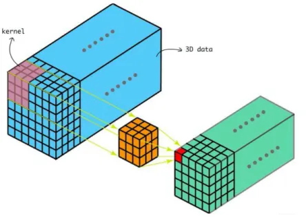
3.3.1 3D-Convolutional layer

Another important introduction made by LeCun was the convolutional layer that, inspired by the human neural network of vision, is the basis for image classification and processing [24].

In an image, nearby voxels can influence each other thus it is important to extract this information.

The convolutional layers allow this with the use of a filter. In this case, the filter is a kernel of a specific size (for example 3x3 or 5x5) that moves across the image. For each point on the image, a value is calculated based on the filter using a convolution operation.

The advantage of this process is that it is possible to reduce the parameters across the network whereas keeping the information of nearby voxels.

After the filters have passed over the image, a feature map is generated for each filter. These are then taken through an activation function, which decides whether a certain feature is present at a given location in the image.

(27)

27

The parameters that can be chosen in Caffe for the 3-dimension convolution layer are the kernel in each size, the stride, the padding, the number of outputs and the activation function of the kernel.

As there is a 3-dimension convolution layer, there are all the others visual layer in their 3-dimension version like the deconvolution and the pooling layers.

All these layers work like their 2-dimension version on the adding dimension.

The deconvolution layer is used in networks like auto encoder network and U-net. It is used to get back the image to the original dimension in tasks like denoising or segmentation, when the output have the same dimension of the input [25] [26].

It works in the opposite way of the convolution layer, generating a bigger image respect the input image of the layer. The deconvolution layer needs 4 parameters:

• Kernel dimension: The dimension of the kernel that will filter the image;

• Stride: How many pixels is moved the kernel during the filtering; • Pad: Number of pixels added to the image for padding purpose;

• Number of outputs: Number of features generated by the

deconvolution layer. (https://towardsdatascience. com/a- comprehensive-introduction-to-different-types-of-convolutions-in-deep-learning-669281e58215)

(28)

28

Figure 7: Graphic representation of 3D-convolution layer

3.3.2 3D-Deconvolution layer

The 3D-deconvolution layer works in the opposite way of the convolutional layer. It takes the same parameters as the convolutional layer:

• Kernel dimension; • Stride;

• Pad;

• Number of outputs.

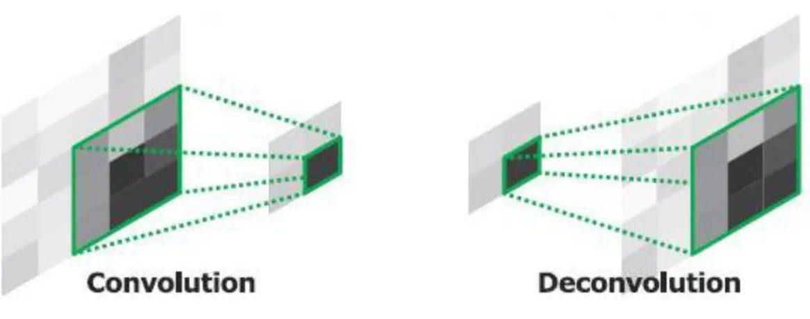
The difference respect to the convolutional layer is that this type of layer augments the dimension of the image. The stride number represent how much the image is going to be augmented during the processing.

(29)

29

The convolutional layer is used in denoising or segmentation task to get back the image to the original dimensions after reducing it in small features by the convolutional layers [27]. (https://towardsdatascience. com/review-deconvnet-unpooling-layer-semantic-segmentation-55cf8a6e380e)

Figure 8: Graphic representation of the differences between convolution and deconvolution layers

3.3.3 3D-Pooling layer

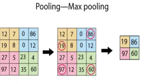
The output features maps can be sensitive to the location of the features in the input. To overcome this problem, pooling layers have been introduced. Pooling layers select specific values on the features maps and pass through the subsequent layers.

This has the effect of making the resulting down-sampled feature maps more robust to changes in the position of the feature in the image, referred to by the technical phrase “local translation in-variance”.

Pooling layers provide an approach to down-sampling feature maps by summarizing the presence of features in patches of the feature map. Two

(30)

30

common pooling methods are average pooling and max pooling that summarize the average presence of a feature and the most activated presence of a feature respectively.

The 3-D pooling layer is the 3 dimensional version of the normal pooling. The pooling is a particular version of the convolution layer where the output of the kernel is the pixel with the higher value. This layer needs 4 parameters:

• Kernel dimension: The dimension of the kernel that will filter the image;

• Stride: How many pixels is moved the kernel during the filtering; • Pad: Number of pixels added to the image for padding purpose;

• Number of outputs: Number of features generated by the

deconvolution layer. (https://principlesofdeeplearning. com/index.php/2018/08/27/is-pooling-dead-in-convolutional-networks/)

(31)

31

3.3.4 Fully connected layer

The fully connected layer connects every neuron of the previous layer with a vector of neurons long has the number of neuron of the layer before. It is use for classification task before the loss layer. (https: //www.xenonstack.com/blog/artificial-neural-network-applications/)

Figure 10: Graphic representation of Fully connected layer

3.3.5 Batch normalization layer

Batch normalization layer normalizes the output of a previous activation layer by subtracting the batch mean and dividing by the batch

(32)

32

standard deviation. This strategy make the back-propagation more stable and more efficient [28].

3.3.6 ReLU layer

The ReLU layer is used in both training and test phase. It is usually used after the convolution or the deconvolution layer to process better no linear features.

Figure 11: Graphic representation of ReLU function

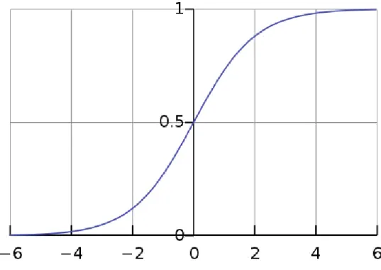
3.3.7 Soft maximum layer

The soft maximum layer is used during the test phase. The soft maximum function is often used in classification task as the last layer because it generates a values of output that always are equal to 1 if are all added.

(33)

33

Figure 12: Graphic representation of SoftMax function

3.3.8 Soft maximum with loss layer

The soft maximum with loss layer is used during the training phase. This layer that calculates for each iteration the loss of the output of the network respect the target and back propagate it to the layer before. It also writes the value in a text file.

The soft maximum with loss layer produce output that are between 0 and 1 and also for this reason is often used when the output of the network is the probability to be of a certain class.

3.3.9 Euclidean loss layer

The Euclidean loss layer takes as input the target of the training and the output generated by the network, compute the loss with the MSE method

(34)

34

and back-propagate it to the previous layer. It also writes the value in a text le.

3.3.10 Accuracy layer

The accuracy layer is used during the training. It compares for every iteration the output of the network with the target, calculates the accuracy and writes it in a text file.

3.4 Test and validation protocols

To validate the result of the project we use the cross-validation test [29]. For the denoising case we used 80 images for the training set and 5 images for the test validation set.

The images were randomly chosen and we repeated the training and the test phase three times with 3 different dataset.

The results are evaluated with a histogram in which is shown the error of the output image of the network respect to the target compared to the error between the input image and the target.

For the denoising case we use a dataset of 135 MRI brain images, 45 for each class.

We perform a cross-validation test also on this dataset: we dived randomly the data set in 90 images for the training and 45 images for the testing, then we train the network and test the accuracy on the test set. We repeated the experiment three times.

(35)

35

The accuracy of the classification is calculated with the classical accuracy index: we take the probability output of the network for right class of the image for every image of the test set, we summed them all together and then we calculated the mean. The accuracy on the test set is calculated for every 2000 iterations and shown in a graph and it is calculated as the mean of the ratio of number of correct predictions to the total number of input samples.

(36)

36

4 Cases

The goal of our study is two folds: • Denoising;

• Differential diagnostic classification.

Even though the ultimate goal would be the later, it was a necessary step to go through the former goal in purpose to really understand the impact of different strategies of layer combination to build a safe classification algorithm.

4.1 Case 1: Denoising

The implementation of the Denoising neural network follows the goal to create a well train image filtering capable to reach the results of an adaptive non-local means denoising process with spatially varying noise levels [30].

An adaptive local mean filter does not make any assumption about the noise distribution across the image, making it a perfect candidate for medical images.

The drawback of this method is the processing takes a long time and are a heavy step in image processing pipelines.

In this section we are going to show that a well designed neural network can reach the level of an adaptive non-local filter using a weak time-stamp.

(37)

37

4.1.1 Dataset

For the denoising case we used 3D structural FLAIR images from 80 subjects, as target the denoised images.

Data augmentation consists of rotation of 9 degrees. The total number of images used as input was 320. Then the images are cropped and saved in HDF5 format as indicate preprocessing paragraph.

Figure 13: Example of MRI used as input

(38)

38

4.1.2 Training hyper-parameters

In this study we used the Adam optimizer (see Appendix for a detailed description).

Adam optimizer requires 4 hyper-parameters: • Learning rate

• Beta1 • Beta2 • X (Epsilon)

For the denoising case we used the values of the hyper-parameters suggested by the original paper of Adam [31].

4.1.3 Neural Network architectures

For the denoising study case we start to build the simplest neural architecture (autoencoder) [32].

As loss function we choose the mean square error, also called Euclidian loss function.

The network architecture consists of: one convolution and one deconvolution with kernel of n x n x n voxels.

Where n is the number of voxels that will define the size of the kernel. For example, If n = 1, the output will have the same dimension as the input image.

(39)

39

The experiment done are the following:

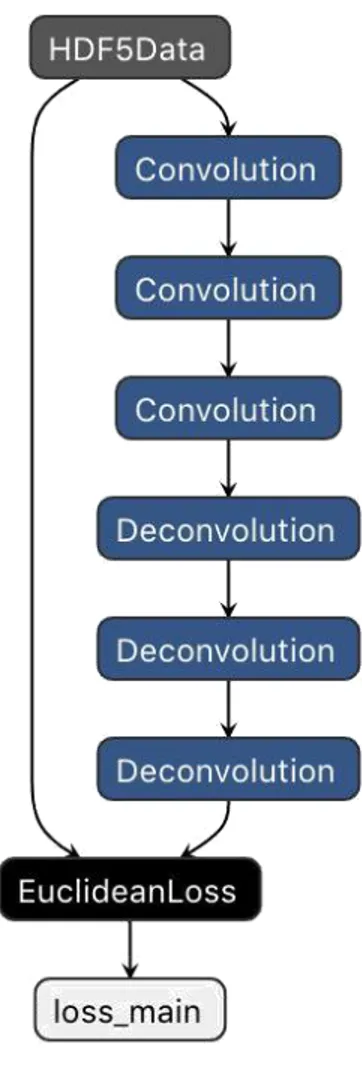
• Model 1 : 1 convolution and 1 deconvolution with kernel’s size of 1, stride of 1, padding of 0 and number of features generated 32. The deconvolution layer has these parameters: kernel of 1, stride of 1, pad of 0 and number of features generated is 1, to get back the image to his original dimension. The input layer is the HDF5 Data layer that take the dataset of HDF5 file and generated input and target of the network. The loss function is the Euclidean loss (or MSE loss) that is the most used when the output are not classes.

(40)

40

• Model 2: 1 convolution and 1 deconvolution with kernel of 3. The second model that we build is identically to the first one with the only exception that the kernel size of the convolutional and deconvolutional layer are of 3 instead of 1. The kernel of 3 is less computational efficient but analyzing the voxels at 3 x 3 x 3 groups has to recognize and reduce better the Gaussian noise.

Figure 16: Scheme of the model 2 of denoising case

• Model 3: 1 convolution and 1 deconvolution with kernel of 5. This model is the same of the first 2, with the only difference that the kernel stride is larger: 5. This larger kernel is less efficient on the computational cost but with a larger kernel maybe is able to reduce the noise better than the model with the kernel of 3.

(41)

41

• Model 4: 1 convolution and 1 deconvolution with ReLU with kernel 3. This model is the same has the second, with the kernel size of 3, with the introduction of ReLU layers before the convolutional and deconvolutional layers. The motivation of the introduction of ReLU layers in the model is that the ReLU function is used to process better no linear features, and in the case of the structure of the brain we are dealing with a lot particular that are not linear at all.

(42)

42

• Model 5: Three convolution and deconvolution. The last model we experiment is a more deep convolution and deconvolution autoencoder. In this new model the parameters of every convolution layers are: stride of 2, padding of 1, kernel size of 3 and the number of features created are 16 for the first, 32 for the second and 64 for the third. The deconvolutional layers have same kernel, padding and stride but the number of features generated is the opposite: 32 for the first, 16 for the second and 1 for the last. The reason why we tried this model is that a deeper convolution processes more features in their details and maybe

(43)

43

going deeper with the convolution and then rebuilding the same image with a deeper deconvolution layer can generate a better denoised image.

(44)

44

4.2 Case 2: Differential diagnostic classification

4.2.1 Dataset

The classification dataset consist in 120 images, 40 for each class that are control, pib negative and pib positive.

The preprocess, if the images consist only in cropping and data augmentation, creating new 3 rotated images from the original.

After data augmentation the hole dataset contains 480 MRI brain images. For the training is used 3/4 of the dataset, the other part is used for the test phase.

4.2.2 Training hyper-parameters

Also for this case we used the Adam optimizer. We start using the hyper-parameters suggested by the paper but then we reduce the learning rate to 0.000001 because 0.001 was to high learning rate for this task.

The batch size for this training is of 4 that is the biggest batch size possible with the memory of the GPU.

4.2.3 Network architecture

The fundamental element to build a image classification neural network are:

• Convolutional layers: they are the first layers that process the image and extract the features that classify the image

(45)

45

• Fully connected layer: after the convolutional layers, a fully connected layer is need to vectorize the image and before the softmax layer

• Softmax layer: it is the last layer and his output are the image’s probability to be of a certain class [33].

We try different architecture to understand which is the best for this task.

From the denoising case we understood that the kernel of three is the best to catch all the features of the brain so we start experiment a convolutional neural network using that kernel size.

The architecture tested are these:

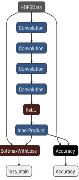
• Model 1: 4 convolution layers. The first model we try to use for the classification task is a 4 convolution layers with one ReLU layer, one fully connected layer and soft max with loss layer. The 4 convolutional layers has stride of 2, kernel size of 3, padding of 1 and the number of features generated is 32, 64, and 128. The ReLU layer is present to process better the non linear characteristic of the brain. The fully connected layer has to vectorize the image features generated by the convolutional layers. This layer then connect with the softmax with loss layer that is the one that calculate the prediction error and back propagate it. The accuracy layer is used during the training only

(46)

46

to write in a text file the values of the accuracy of the image to be classified in the right class by the network.

(47)

47

• Model 2: 4 convolution layers with first layer stride of 1. The second experiment for the classification task is the same network as the first but with the first convolution layer that has a stride of 1 and padding of 0. This change makes the first layer analyze the features of the brain image in the original dimension. This is less computational efficient because increase the number of parameters to train, but analyzing the image in the original dimension it can also extract more features that characterize the brain class respect reducing the dimension of the image form the first convolution. After the 3 convolutional layers there are a ReLU, to analyze better the non linear part of the brain, the fully connected or inner product layer and the soft max with loss layer as the cost function.

(48)

48

Figure 21: Scheme of the model 2 of classification case

• Model 3: 4 convolution layers and ReLU. The third experiment consist in a network similar to the previous one but with the introduction of ReLU layer after every convolutional layer. The ReLU layer is used to process non linear and has the brain is

(49)

49

made only but non linear details, the introduction of the function after every convolutional layer can improve the processing and the result of our model. The parameters of the convolutional layers are the same of the second network and the loss function used is still softmax with loss.

(50)

50

• Model 4: 4 convolution layer, ReLU and pooling. The last experiment we try is the introducing of the pooling layer. In this case the stride of the convolutional layers is left at 1 and the pooling layers make the work to reduce the image of half. The pooling layer is often used in the image processing task in a block with first convolutional layer and ReLU. We reproduce this in our model putting together three blocks composed by convolutional, ReLU and pooling. After the 3 blocks there is a fully connected or inner product layer before the soft max with loss layer to calculate the loss and the accuracy layer to calculate the prediction accuracy during the training.

(51)

51

(52)

52

• Model 5: 4 convolution layer, ReLU and batch normalization. In this experiment we introduce a batch normalization layer after every convolutional and ReLU layer to make the training more stable and effective.

(53)

53

5 Result

5.1 Case 1: Denoising

For the denoising case the image are evaluated as the difference of the output image, generated by an image non contained in the training set, respect the target image. This error is compared with the error of the input image respect the target image. To graphically show this result we build a histogram the show the two errors.

On the next result part is also showed the loss function during the training to analyze how the loss function decrease during the training.

• Model 1: 1 convolution and 1 deconvolution with kernel of 1. Low performance, the kernel is to small and cannot improve the gaussian noise present in the MRI images.

Figure 25: Loss function during the training model 1

The loss function shown in the previous images show that the number of iterations needs to reduce the loss function to his minimum are only

(54)

54

around 500, but the result of the network on a test image show that the network is only able to recreate the image as the input of the network.

Figure 26: Image generated by the network model 1

The histogram representing the error of the output image generate by the network respect the image (green) versus the error of the input image respect the target (blue), shows that the model is not able to reduce the noise of the image and generate a better image.

Figure 27: Histogram representing the error of the input(blue) and the output(green) respect the target model 1

(55)

55

• Model 2: 1 convolution and 1 deconvolution with kernel of 3. Good result and very efficient network. The dimension of the kernel is sufficient to reduce the white noise and the number of parameter is not increase to much respect the one with kernel 1.

The loss function and the output generate by this network shown better result respect the network with kernel of 1. The loss function graph shows that the function reaches a smaller value, the number of iterations to reach the minimum is close to the one of the previous experiment. The output generated by the trained network shows a better image respect the input one in which the Gaussian noise is reduced, the quality of the output image is still not good as the target image.

(56)

56

The histogram shows that the output image has a smaller error compared with the previous experiment.

Also the big part of the error become more close to the center of the histogram that represent a small error.

(57)

57

• Model 3: 1 convolution and 1 deconvolution with kernel of 5. Same result with kernel of 3 but the network is less efficient the number of parameters to train are more.

The performance of the network with the kernel of 5 is the same of the one with kernel of 3 in term of result, instead in term of computational performance is lower. This can be seen in the loss function graph in which the number of iterations need to reach the minimum are bigger respect the previous experiments, but the value reach and the outputs of the network are the same of the experiment with the kernel of 3. The reason why this model is less efficient in term of computational performance is that a kernel of 5 has more parameters to t respect a kernel of 3 and it not shows better result to justify his use.

(58)

58

The histogram that compares the output of the target respect to the target shows that the quality of the image generated is the same of the previous experiment. Also from the previous image, comparing it with the one of the experiment with kernel of three, we can see that the white noise is reduce and the image quality is the same as the previous experiment.

(59)

59

• Model 4: 1 convolution and 1 deconvolution with ReLU with kernel 3. After choosing the best kernel size we introduce a ReLU layer after the convolutional and the deconvolution. The ReLU layer improve the result of the network.

From the next image we can see that this experiment shows the best result in term of quality of the image generated. The introduction of the ReLU layers helps the network to understand and reproduce smaller and less linear features.

The graph of the loss function during the training shows that the number of iterations too reach the minimum value is still small, around 2500 iterations. This means that our model is also computation efficient.

(60)

60

The histogram that compares output image of the model respect to the input shows that the error is smaller respect the other case, this means that our output image is very close to the target one and that the Gaussian noise is drastically reduced.

This can be notice also comparing the visual image generated by the networks in the different experiments.

(61)

61

• Model 5: 3 convolution and 3 deconvolution. The 3 level of convolution and deconvolution shows same result as the network before, but the number of iterations needed is 10 times more.

The last model that we experiment shows that it needs a bigger number of iterations to reach his minimum.

The reason why is that this model has 3 level of convolution and each generated more features respect the previous layer, this make the model has an increased number of parameters to train respect to the other experiment and so it needs at least 100’000 iterations to reach his minimum. The result shows a image that is not good as the one of the previous experiment but still the Gaussian noise is reduced and the image is better respect the input one.

(62)

62

The histogram shows that the error is bigger respect the one of the previous experiments. The reason why is that using a small dataset we cannot deploy a big network with a big number of parameters because is generated an over fitting problem caused by the too high number of parameters to fit.

(63)

63

5.2 Case 2: Differential diagnostic classification

• Model 1: 4 convolution layers. The training of the first network experiment shows that this network is not able to classify and recognize the differences between the 3 groups. This can be seen in both the loss graph, in which the loss function is not stable and decrescent, and in the accuracy one, that not reach the 70%.

(64)

64

In both the graph we can also notice that the training is not stable and continue to oscillate between a minimum and a maximum. The reason why is that the architecture of this network is not compatible with the task that we want to implement.

(65)

65

• Model 2: 4 convolution layers with the first of stride of 1. The second experiment shows better result. Processing the image with the original dimensions in the first layer the network is able to classify and recognize the difference of the training set images. The loss function is still not stable but is decrescent, the same for the accuracy that reach very good value but is not stable during the training.

This network shows to be able to classify the image of the training set but, using too much iterations to reach the minimum for the loss function and the maximum for the accuracy function, there will be the overfitting problem if we want to use the model with a new data not present in the training set. The reason why is that we use too many times the same image during the training to reach that number of iterations and the consequence

(66)

66

is that the model is too much trained on the training set images and is not able to generalize to image not present in the training set.

Figure 43: Accuracy during the training model 2

• Model 3: 4 convolution layers and ReLU. Introducing the ReLU layer after every convolution one make both the loss function and the accuracy more stable during the training.

(67)

67

This model shows a more stable and efficient training. The loss function decreases stable till reach his minimum. The opposite for the accuracy function that increase stable till reach his maximum of one. As the same of the denoising case the introduction of the ReLU layers after every convolutional blocks, makes the network more able to recognize the smaller and non linear details of the MRI brain scan.

(68)

68

• Model 4: 4 convolution layers, ReLU and pooling. The introduction of the pooling layer not improve the performance of the network but it makes it worst.

As the same of the denoising case, the introduction of the pooling layer does not help the network to improve the result but instead makes it worst.

(69)

69

This can be notice by both loss function and accuracy graph, they are less stable and also the values that they reach are smaller for the accuracy and bigger for the loss function.

• Model 5: 4 convolution layers, ReLU and batch normalization. The introduction of the normalization layer produces the more stable and effective training.

(70)

70

The introduction of the batch normalization layer produces the best result of all experiments. The two graphs show that the values and the stable of the two functions are superior with this network respect the other case. The reason why is that using a patch based training, the process of normalization of the images after every convolutional block, makes the network more able to classify the images in the right group.

(71)

71

5.2.1 Test phase

The last model is been test with the cross-validation accuracy test described in the methods section. The reason why we test the accuracy on all the training iterations is to understand which is the best number of iterations for the model and when over fitting problem on the test data start to influence the model.

(72)

72

Figure 50: Accuracy on the test set every 2000 iterations model 5

The graph shows that the number of iterations to reach the maximum accuracy on the test set are 10’000, this mean that our model is computational efficient.

The value of accuracy reach is low 0.63, but also from the literature we see that the number of images that we have is too small to reach better result in term of accuracy on the test set.

After the 20’000 iterations the overfitting problem starts to affect the model and the performance bringing it back till reach the 0.54.

The reason why is that the small number of images are used too much times during the training and so the overfitting problem start very early to affect the CNN during the test phase.

(73)

73

6 Discussion and conclusion

In this part I will introduce the main findings of this project and explain the innovative contributions and relevant aspects of the implemented methods.

Then I will tell about the limits and possible improvements for this work and i will end the chapter with a conclusion.

6.1 Main findings

In the next picture shows the result for the classification case.

In the first column there are the model, in the second the accuracy reached during the training and in last column shows the accuracy on the test set.

For the first and third model the accuracy is not calculated because the accuracy on the training set is too low to work on the test set.

(74)

74

The best CNN model that we created is still not able to perform a good classification on our clinical case.

The reason why is that the number of data is too small to create a convolutional neural network model that is then able to generalize to data that are not present in the training set.

Also if the main goal of the thesis is not was not reached during our experiment we understood which type of network architecture was the best to create the most performant model.

For what concern the network architecture we discover that the best block of layer to perform the classification task is composed by convolutional layer, ReLU layer and batch normalization layer in series.

The architecture that performs the best result is composed by the block previous described repeated for 4 times but with a small number of features created.

The 4 blocks of layers perform a deep processing of the image that is needed to recognize all the features of the brain. The few numbers of features created is for the overfitting problem.

With a small data set the overfitting problem become more relevant. With a low the number of features created there are less parameter to fit and this balance in part the problem of have a small dataset regarding the over fitting problem.

The add of the ReLU layer shows increase the efficiency of the artificial neural network on both the denoising case and the classification case.

The reason why is that this layer produce a better processing of the non linear features.

(75)

75

The details of the brain are all non linear structure and so the ReLU layer improve the performance of the network.

The batch normalization layer improves also the efficiency of the model. The reason is that all the images has different intensity caused by different external factor and so a normalization of the batch make all the image with the same threshold and more detectable by the other layer.

Another discover about the network is that the pooling layer, if insert in the basilar block, do not help the model to classify better the MRI brain scan, but produce worst result both in the classification case and in the denoising case.

6.2 Innovative contributions and relevant aspects of

the implemented methods

The most important contribution that we bring is the best type for the most efficiency convolutional neural network for image classification with a small dataset of brain MRI.

The network consists in 4 blocks repeated in series, the block is composed by:

• 3D-convolution layer; • ReLU layer;

(76)

76

To make the network effective also with a small dataset the number of features generated by the network has to be low because in this way we overcome the overfitting problem.

The pooling layer, if added to the principal block, produces worst result so we suggest to do not use this layer in visual processing task instead use a convolutional layer with the stride of two to reduce the dimension of the image during the creation of deep features.

6.3 Limits and possible improvements

The limits of the project are that with a small dataset of 30 images for each class is very difficult crate a model that can classify the image with an high accuracy.

For now is not present a dataset that contains more images about the 3 class the we try to classify.

The possible improvements that I would like to try to implement is to download the ADNI dataset that contain a more then thousand brain MRI, but divided only in two class (Alzheimer and control), and try to see which is the minimum number of images necessary to produce a model with a accuracy of at least of 90% on the test set.

This experiment can show us which is the minimum number of images that we need to build a good classifier also with the 3 classes.

Another improvements that I would like to try is to use the transfer learning.

(77)

77

Use the information stored by the network in the first case training for the second case.

To do that we create a model that has 2 output, in specific we add together the most efficient model of the denoising case with the most efficient model of the classification case.

Then we train the model on the denoising training set.

Finish the first training we make the second with our reset all the weight and biases of the network. This technique may allow to overcame the over fitting problem and generate a model more efficient also with the dataset present today.

6.4 Conclusion

The model generated was not able to predict the test data with an accuracy superior of the 70%.

The reason why is that the ANN technique need a number of data that is not always present especially in the medical field.

We understood and reported some architecture details that make the network more efficient also with a small number of data.

My work at UCSF is still not finish and we will try other implementation and technique in this field of machine learning like the transfer learning to implement a better model.

(78)

78

7 Appendix

In this part I will introduce the artificial neural network and all his components.

The main components of neural networks are the layers, the cost function and the back-propagation algorithm.

These concepts are before introduced in more general way and then I start to enter in the details also with the mathematical formulas.

7.1 Artificial Neural Networks

Artificial Neural Networks (ANN) are computational models that have emerged as a result of a simulation of the biological nervous system to perform a variety of tasks.

As a resemble of the biological system, ANNs acquire knowledge through a learning process.

ANNs have been around for 50 years and basically they are a type of machine learning used in supervised learning.

Machine learning used algorithms to extract information from data and represent it in some type of model.

We then can use these models to infer things about other data we have not yet modeled.

Compared to the classical machine learning, ANNs attempts to create a network of “nodes” working in parallel as we assume the human brain does.

(79)

79

The first neural network was introduced in 1957 by Frank Rosenblatt as a simplified model of a neuron called the perceptron [34].

The perceptron is a linear-model binary classifier with a simple input-output relationship. The perceptron receives multiple input signals at multiplied by their weights 𝑊_𝑖, sums them up, and feeds an activation function g(x) that defines an output y.

During the learning phase, the perceptron changes the weights to minimize the error until all the record inputs are correctly classified. (https://www.simplilearn.com/what-is-perceptron-tutorial)

Figure 52: Main Processing Unit

The main limitation of the perceptron was its inability to solve nonlinear problems. Only years later, in 1974, the first non-linear processing capabilities of ANNs were reported and since then the interest of the

(80)

80

scientific community increase exponentially boosted with the increase in computational power together with the advances in computer technology [35].

ANNs are inspired by the biological neuron with three principal components:

• Dendrites: input connections with other neurons;

• Cell body: the central part of the neuron when the signal is processed;

• Axons: the output connections to other neurons.

ANNs are indeed represented as a set of nodes called neurons and connections between them. The connections have weights and represent their strengths.

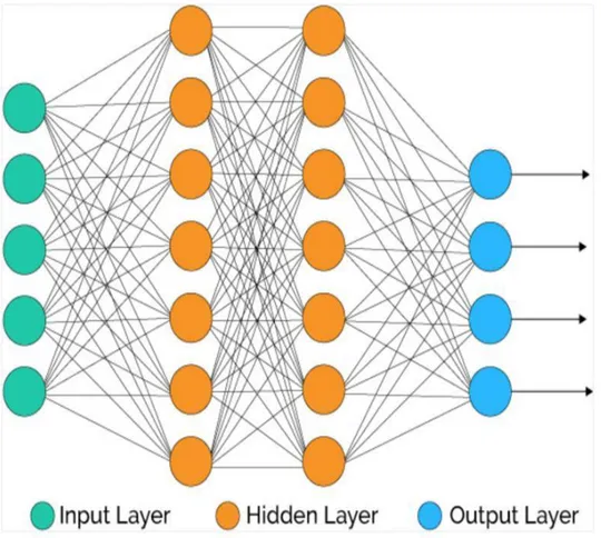
The basic architecture of a neural network has 3 layers:

• Input layer: this layer is the interface with the environment; • Hidden layer: this is the computational layer;

• Output layer: this is the layer where the output is stored. Different neural network architecture can be built using multiple layers. In particular, the use of multiple hidden layers could help in solving complex problems. This type of architecture defined the so-called

multilayer Feed-Forward networks.

( https://www.xenonstack.com/blog/artificial-neural-network-applications/)

(81)

81

Figure 53: Example of multilayer feed-forward network implementing two hidden layers

Each layer has one or more artificial neurons which differs by each other for the activation function that serves to the specific purpose of the layer.

(82)

82

7.2 Activation functions and Forward Propagation

Activation functions control the behavior of the artificial network. Depending of the application, multiple activation functions are available. Most of the time the activation shape follows the sigmoid profile, simulating the ring process of neurons.

The most common functions are:

• Linear: function where the dependent variable has a linear relationship with the independent variable;

• Logistic: function that converts independent variable of near-infinite range into simple probabilities between 0 and 1. Its characteristic is then to reduce values or outliers without removing them;

• TanH: a hyperbolic trigonometric function, it transforms the independent variable to a range between -1 and 1. Its advantage is that can deal easily with negative number;

• SoftMax: generalization of logistic regression, it can be applied to continuous data and can contain multiple decision boundaries. This function is often used in a classification problem;

• Rectified linear unit (ReLu): a function that activates a node only if the input is above a certain positive quantity. Above this threshold, the function has a linear relationship with the dependent variable [36].

3D CNN for classification of brain MRI