POLITECNICO DI MILANO
SCHOOL OF INDUSTRIAL AND INFORMATION ENGINEERING
Master of Science in Mechanical Engineering
An experimental method for the estimation of the
adhesion coefficient and the running resistance of a train
Supervisor:
Prof. Juan de Dios Sanz Bobi
Co-Supervisor:
Prof. Stefano Bruni
Candidate:
Antonino Spinalbese
ID: 842132
3
Abstract
The formulas of the current running resistance are derived historically from the experimental studies of the first part of the XX century. Now, these methodologies are still effective, but it is important to investigate this area due to the enormous transformation of the actual rolling stock, related to the progress of the technology. Each manufacturer of the locomotive calculates the resistance in a different way and sometimes it is nearly impossible to compare the resistance of two different companies. In addition, the ideal test done for the manufacturer does not reproduce accurately the real railway operation. For all these reason, Renfe, the Spanish state-owner railway company would like to verify and control these equations, in order to have the real effective resistance of the own rolling stock and therefore increase, if it possible, the load towed and the operation of the freight sector. So, the objective of the following study is to calculate the running resistance of a particular locomotive depending on the load and guarantee its worth. On the other side, in this study it is estimated the wheel-rail adhesion coefficient at starting condition in three different configurations: dry, wet and with oil. The main principle and characteristic of this work is the on-site measurements done during the experimental tests. In contrast, it is developed a simulation of the configuration at different velocity in order to study the aerodynamic profile of it. With this tool, it is possible to obtain a comparison between the aerodynamic resistance measured in the test and the one that is calculated through the software. As result, the aerodynamic resistance is decoupled from the other parts of the running resistance and it can be calculated through the simulation, saving money and time. This method could be considered as a model and be extrapolated to other rolling stocks.
Keywords: Running resistance, adhesion coefficient, test field, data gathering, CFD simulation.
4
Sommario
Le formule attuali della resistenza all’avanzamento derivano storicamente da alcuni studi sperimentali fatti nella prima parte del XX secolo. Ora, le metodologie usate per calcolarle sono tuttora efficaci, ma risulta di vitale importanza investigare su questo tema dovuto alle grandi trasformazioni che ha subito il materiale rodante grazie allo sviluppo tecnologico degli ultimi anni. Per di più ogni produttore di locomotive calcola la resistenza in maniera differente e comparare i risultati risulta difficile. Inoltre, i test effettuati idealmente da questi produttori non riproducono fedelmente la realtà del mondo ferroviario. Per tutte queste ragioni, Renfe, la impresa ferroviaria pubblica spagnola ha voluto verificare e controllare queste equazioni, per avere un reale valore della resistenza del proprio materiale rodante e in questo modo aumentare, dove possibile, il carico trasportato e di conseguenza migliorare le operazioni del settore mercantile. Di conseguenza l’obiettivo principale di questo studio è quello di calcolare la resistenza all’avanzamento di una particolare locomotiva in funzione del carico e garantire la sua validità. Dall’altro lato, viene anche calcolato il coefficiente di aderenza in partenza in tre diverse configurazioni: secco, bagnato e con olio. La principale caratteristica della tesi è rappresentata dalle misure fatte in situ nei due rispettivi test. In contrasto con questa parte sperimentale, è stato sviluppato una simulazione della composizione a diverse velocità per studiare e caratterizzare il suo profilo aerodinamico. Con questo strumento, è possibile ottenere un confronto tra la resistenza aerodinamica misurata nel test e quella calcolata attraverso il software. Come risultato, la resistenza aerodinamica risulta disaccoppiata dalle altre parti della resistenza all’avanzamento e può essere calcolata con la simulazione, risparmiando denaro e tempo. Questo metodo potrebbe essere considerato come un modello e estrapolato per altre composizioni e configurazioni.
Parole chiave: Resistenza all’avanzamento, coefficiente di aderenza, ambito di test, raccolta di dati, simulazione CFD.
5
Table of Contents
1.
Introduction, objectives and methodology... 13
2.
State of Art ... 17
2.1 Introduction: the longitudinal dynamic ... 17
2.2 Running resistance in straight condition: Davis’s Formula ... 20
2.2.1 Mechanical running resistance: A term ... 22
2.2.1.1 Resistance due to rolling ... 23
2.2.1.2 Resistance due to internal friction ... 24
2.2.1.3 Typical values of the mechanical resistance ... 24
2.2.2 Running resistance due to the entrance of air: B term ... 27
2.2.3 Aerodynamic resistance: C term ... 29
2.2.3.1 The drag coefficient... 31
2.2.3.2 Considerations in order to reduce the aerodynamic resistance ... 32
2.2.3.3 Aerodynamic drag in tunnels... 33
2.2.3.4 Modification and adjustment criteria for the aerodynamic drag ... 34
2.2.3.5 Variation of the aerodynamic coefficient with the train length ... 35
2.2.3.6 Variation of the aerodynamic coefficient with pressure and temperature ... 38
2.3 Typical formulas of the running resistance in straight in open air without wind ... 40
2.3.1 Trains of variable composition. Simple formulas ... 41
2.3.2 Non-deformable composition trains ... 42
2.3.3 Running resistance values for different trains ... 42
2.3.4 Relative influence of each of the factors of the running resistance ... 46
2.4 Running resistance in straight condition: Strahl’s formula ... 47
2.5 Longitudinal force due to gravity: gravitational resistance ... 49
2.6 Traction force and adherence ... 50
2.6.1 The traction force ... 51
2.6.2 The adherence ... 52
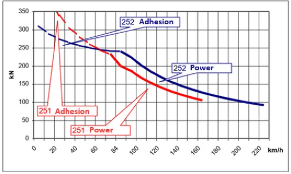
2.6.2.1 Incidence of the adherence on the traction... 54
2.6.2.2 Adhesion values... 56
3.
Description of the tests ... 59
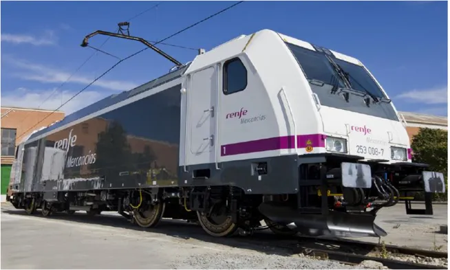
3.1 Locomotive: Bombardier TRAXX DC ... 60
3.1.1 Data Recorder of the locomotive: Teloc ... 62
3.2 Wagons ... 63
3.3 Measuring equipment ... 65
3.3.1 Data recorders ... 65
3.3.2 Current-measuring clamps ... 66
3.3.3 Accelerometers ... 68
3.3.4 Manometers Pitot tubes ... 69
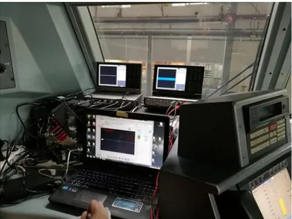
3.4 First test day – February 27 ... 71
3.4.1 Scheme of the measurement equipment ... 73
3.5 Second test day – May 5 ... 73
6
4.
Calculation and analysis results ... 81
4.1 Process of calculation ... 82
4.1.1 Conversion factors ... 82
4.1.2 Movement equation ... 83
4.1.3 Assumption and considerations ... 86
4.1.4 Method 1 ... 87
4.1.5 Method 2 ... 89
4.2 Graphics ... 90
4.3 Running resistance calculation ... 93
4.3.1 Analysis of the data of May and list of test run ... 93
4.3.2 Graphical representation of the essays ... 94
4.3.3 Treatment of the data ... 100
4.3.4 Regression Analysis: Polyfit results ... 101
4.3.5 Regression analysis: Curve fitting results ... 103
5.
Simulations ...107
5.1 The measure of the locomotive ... 107
5.2 The creation of the 3D model ... 109
5.3 The CFD simulations ... 113
5.3.1 SolidWorks Flow Simulation ... 113
5.3.2 ANSYS Fluent ... 117
5.3.3 The final comparison... 129
6.
Conclusions and future research lines...133
6.1 Conclusions... 133
6.2 Future research lines ... 135
7
List of figures
Figure 1 – Variation of the coefficient C with respect to the length of the train [18] ... 37
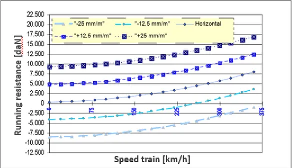
Figure 2 – Running resistance in horizontal and in straight condition for different types of trains ... 45
Figure 3 – Relative weight of the components of the running resistance and of the gravitational (for this case is 11.2 mm/m for a Talgo 350) ... 46
Figure 4 – Resistance due to the gravity ... 49
Figure 5 – Total running resistance of a high-speed train Talgo 350 with different slopes ... 50
Figure 6 – Traction force limited by the power and the adhesion in the locomotive 251 and 252 ... 55
Figure 7 – Locomotive S253 used for the freight sector with which the tests have been realised ... 60
Figure 8 – Lateral view of the locomotive ... 61
Figure 9 – Example of the Teloc data... 63
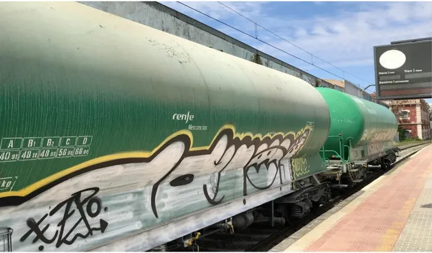
Figure 10 – Photo of the tank wagons taken in Alcázar de San Juan on the test day of May ... 64
Figure 11 – Scheme of the tank wagon ... 64
Figure 12 – Recorders GRAPHTEC Corporation used for the data gathering of the tests ... 65
Figure 13 – Installation of the data recorders in the locomotive cabin... 66
Figure 14 – Configuration of the current clamps ... 67
Figure 15 – Installation of the current clamp in one of the phases of the motor ... 67
Figure 16 – Accelerometer used in the tests ... 68
Figure 17 (a, b) – Installation of the accelerometers in the first wagon (left) and in the locomotive (right) ... 69
Figure 18 – Manometers Pitot tubes used during the full day test of May ... 70
Figure 19 (a, b, c) – Wheel and rail are impregnated with oil to perform the last start test ... 72
Figure 20 – The composition at the Alcázar de San Juan (Ciudad Real) station ... 74
Figure 21 – Arrangement of the Pitot tubes on the front and on the later side of the locomotive ... 76
Figure 22 – A detail of the installation of the Pitot tube on the front of the locomotive ... 76
Figure 23 – The fluid flow around the composition during the motion ... 78
Figure 24 – Flow chart of the phases realized in the work ... 82
Figure 25 – Longitudinal dynamics of a railway vehicle ... 84
8
Figure 27 – Typical values of the adhesion coefficient at start ... 86
Figure 28 – Graphic of the values recorded by the longitudinal accelerometer of the locomotive during a start test ... 91
Figure 29 – Graphic of the values recorded by the longitudinal accelerometer of the first wagon during a start test ... 91
Figure 30 – Record of the speed and of the column Traction_Active of the Teloc during a start test ... 92
Figure 31 – List of files generated during the second test day... 93
Figure 32 – All the 26 essays done during the test (speed-time curve) ... 99
Figure 33 – Regression Curve fitting for the second method ... 103
Figure 34 – Regression curve fitting with the first method ... 104
Figure 35 – Regression Curve fitting for the second method (modified)... 105
Figure 36 – Scheme of the locomotive ... 108
Figure 37 – Half CAD model of the locomotive ... 110
Figure 38 – Section of the CAD model ... 110
Figure 39 – Component of the bottom part of the locomotive ... 111
Figure 40 – The entire 3D model of the locomotive ... 111
Figure 41 – The locomotive model with the track ... 112
Figure 42 – CAD model of the total composition with the track ... 112
Figure 43 – Absolute pressure on the locomotive surface at 100 km/h ... 114
Figure 44 – Behaviour of the air flow impacting the composition in the plane of symmetry 115 Figure 45 – Velocity of the air flow impacting the composition ... 115
Figure 46 – A detail of the air flow for the front section ... 116
Figure 47 – A detail of the rear section of the composition ... 116
Figure 48 – The locomotive and the airbox in the DesignModeler section ... 118
Figure 49 – Details of the mesh configuration ... 119
Figure 50 – Another control volume: Trainbox ... 120
Figure 51 – The effect of the Trainbox and of the body sizing function ... 120
Figure 52 – Details of body sizing ... 121
Figure 53 – Statistics of the mesh ... 121
Figure 54 – Mesh metrics: number of elements with respect to the skewness ... 122
Figure 55 – Setting parameters for the first 100 iterations ... 123
Figure 56 – Scaled residuals graph ... 125
Figure 57 – Drag coefficient convergence history ... 125
9
Figure 59 – Pressure contour on the locomotive surface at 100 km/h ... 126
Figure 60 – Velocity streamline of the air at 100 km/h at front section... 127
Figure 61 – Velocity streamline of the air at 100 km/h at rear section ... 127
Figure 62 – The entire velocity streamline at 100 km/h ... 128
Figure 63 – Flux report ... 128
10
List of tables
Table 1 – Different values of the drag coefficient for various transport vehicle ... 31
Table 2 – Variation of the C coefficient and of the density respect to the pressure and the temperature ... 39
Table 3 – Absolute and specific coefficients of running resistance formulas in several conventional trains ... 42
Table 4 – Absolute and specific coefficients of running resistance formulas in several high-speed trains... 43
Table 5 – Coefficients A, B and C of the Davis formula ... 44
Table 6– Adjusting of the Davis formula multiplier factor ... 44
Table 7 – Coefficients A, B and C of the modified Davis formula ... 45
Table 8 – Running resistance in horizontal and in straight condition for different types of trains ... Errore. Il segnalibro non è definito. Table 9 – Coefficients A and C of the Strahl’s formula ... 47
Table 10 – Scheme of the instrumentation equipment with the respective channel of the recorder ... 73
Table 11 – Scheme of the instrumentation equipment with the respective channel of the recorder ... 73
Table 12 (a, b, c, d) – Characteristics of the line of the test ... 75
Table 13 – Scheme of the instrumentation equipment with the respective channel of the recorder ... 79
Table 14 – Scheme of the instrumentation equipment with the respective channel of the recorder ... 79
Table 15 – The conversion coefficients for the Pitot tubes ... 82
Table 16 – The conversion coefficients for the accelerometers ... 83
Table 17 – The conversion coefficient for the current clamps ... 83
Table 18 – Values of the adhesion coefficient calculated with the method 1 ... 88
Table 19 – Values of the adhesion coefficient calculated with the method 2 ... 89
Table 20 – Comparison of the values of the adhesion coefficient calculated with the two methods ... 90
Table 21 – Example of the variables collected... 101
11 Table 23 – Results of the regression analysis using Curve fitting function for the second method ... 103 Table 24 – Results of the regression analysis using Curve fitting function with the first
method ... 104 Table 25 – Results of the regression analysis using Curve fitting function for the second method (modified) ... 105 Table 26 – The drag and the lift force calculated by SolidWorks Flow Simulation ... 117 Table 27 – Comparison between the pressure simulated and the one measured during the test ... 129 Table 28 – The pressure measured during the test at different range of velocity... 129 Table 29 – Drag resistance comparison ... 131
13
1.
Introduction, objectives and methodology
The formulas of the current running resistance are derived historically from the experimental studies of the first part of the XX century. Now, these methodologies are still effective, but it is important to investigate this area due to the enormous transformation of the actual rolling stock, related to the progress of the technology. Each manufacturer of the locomotive calculates the resistance in a different way and sometimes it is nearly impossible to compare the resistance of two different companies. In addition, the ideal test done for the manufacturer does not reproduce accurately the real railway operation. For all these reason, Renfe, the Spanish state-owner railway company would like to verify and control these equations, in order to have the real effective resistance of the own rolling stocks and therefore increase, if it possible, the load towed and the operation of the freight sector. So, the objective of this study is to calculate the running resistance of a particular locomotive depending on the load and guarantee its worth. The formula is not only crucial for the calculation of the load that can be towed, but this is intrinsically connected also to the energy consumption. A reduction of the running resistance provokes a reduction of the energy consumption for the same load towed. On the other side, in this study it is estimated the wheel-rail adhesion coefficient at starting condition in three different configurations: dry, wet and with oil.
The main principle and characteristic of this work is the on-site measurements done during the tests. In contrast, it is developed a CFD simulation of the configuration at different velocity, in order to study the aerodynamic profile of it. With this tool, it is possible to obtain a comparison between the aerodynamic resistance measured in the test and the one that is calculated through the software. As result, the aerodynamic resistance is decoupled from the other parts of the running resistance and it can be calculated through the simulation, saving money and time, avoiding to calculate it with an experimental test. This method could be considered as a model and be extrapolated to other existing rolling stocks.
14 So, the procedure to follow is: to do a treatment and study of a series of real data obtained from measurements done experimentally with a particular rolling stock. With this experimental data it has been possible to estimate the adhesion coefficient and the running resistance formula.
To get the final results a series of tasks are carried out: firstly, the description of the tests, from the design to the execution of the same, going through the establishment of the requirements of the instrumental material for data collection. Second, the development of a theoretical approach for a rigorous treatment of the data obtained, in order to perform a proper analysis of them. This will allow to establish the most accurate calculation methods for the estimating of the values of said parameters. Third, the creation of a 3D CAD model of the rolling stock in order to study the aerodynamic profile and to get the flow simulation at different velocity. Fourth, the CFD simulations with two different software in order to compare and validate the results of them with the experimental data. The software used in this last part of the project are: SolidWorks, that is used to create the 3D model of the composition; SolidWorks Flow Simulation, an intuitive Computational Fluid Dynamics (CFD) solution embedded within SolidWorks 3D CAD that enables to quickly and easily simulate the flow of air at different velocity around the model; and ANSYS Fluent, another CDF software that can simulate the same simulation and it is used to have other estimation of the aerodynamic resistance.
In conclusion, the entire work is realized in order to understand if, the fundamental variables that intervene in the equation of running resistance can be calculated by the railway company itself, through a series of experimental tests or through a virtual simulation. In this way the companies can estimate properly the load towed and also the energy consumption to move that load. This would be of benefit for all the freight sector.
This document describes the way to proceed in the realization of the entire project: after the introduction, in the second chapter is delineated the state of art of the running resistance formulas and their characteristics; in the third the experimental test and the data gathering are described with all the components and the measurements equipment; in the fourth the assumptions and the calculations done are characterized, while in the fifth chapter the studies done in
15 the simulations are reported with the final comparison. The last part outlines the conclusions of the project and the future research lines.
The whole project has been developed with the support of the “Fundación de los Ferrocarriles Españoles” (FFE) and the “Escuela Técnica Superior de Ingenieros Industriales” of the “Universidad Politecnica de Madrid (UPM)”.
17
2.
State of Art
In this chapter, the equations that currently define the values of the running resistance and the parameters that control them, are studied, with a special emphasis on the mechanical resistance and on the aerodynamic one. All the variables that affect the resistance are described in depth, parameterizing the different contribution of the elements of the rolling stock and its environment. The speed, for example, is the most critical variable in terms of aerodynamic drag. In the same way, the phenomenon of adhesion and contact between wheel and rail is also studied. These fundamental concepts serve as a basis for the subsequent analysis of the data obtained in the records for the estimation of the adhesion coefficient at start.
2.1 Introduction: the longitudinal dynamic
In this section, it is described the longitudinal dynamic of a train. In other words, it is explained the movement of the train in the direction of the track and the forces that affect this movement. It is a fundamental area of study for the railway operation, since on it, are based important aspect as the calculation of travel times, the energy consumption or the determination of the maximum load.
Several and very different forces act on a train, but in this work, just the longitudinal components of the forces (on the longitudinal axis of the track) are described. The other components are not considered since they are studied in the domain of the infrastructure or in the stability domain. For what concerned the longitudinal forces applied on a train, there are two different types:
18 • Passive forces, which are the ones that do not depend on any action of the train
itself. Passive forces are, for example, the running resistance (in straight and in curve) or the gravitational force;
• Active forces, which are the forces produced by the train, in particular, they are the traction and braking forces. These forces cause an acceleration or a deceleration of the mass of the train allowing (or stopping) its movement.
It is called running resistance the resultant of the forces that oppose the movement of the train in the longitudinal direction of the track, without considering the gravitational, traction and braking forces. It is always a negative force (opposing the movement). More specifically, the running resistance is the projection, on the longitudinal axis, of different passive forces that act on the train and that are of different character. Among them it can be possible to distinguish the following:
• Friction force between the wheels and the rails;
• Internal friction forces in the moving and rotating parts of the train;
• Force necessary to accelerate the air that enters in the train (for the refrigeration of the engines and for the air renewal of the interior);
• Aerodynamic drag, which consists of pressure and friction resistance, and it is especially important at high speed;
• Friction force due to the contact between the flange of the wheel on the rail in curves.
The total running resistance can be decomposed according to Brina [1] and Toledo et al. [2] in two parts:
• Running resistance in straight condition 𝑅𝑎𝑟, (that is different in open air and in tunnel, where the aerodynamic effects increase the resistance as it is described later);
• Running resistance in curve 𝑅𝑎𝑐 (it is not a topic of this work) and the resistance due to a gradient.
Naturally, the total running resistance 𝑅𝑎𝑡 is the sum of the previous ones:
19 This total resistance varies almost constantly, because the train passes through straight alignments and curves of different radius successively. Also, it must be taken into account that the running resistance in straight condition is dependent on the speed of the train, so any variation of the real velocity leads to a variation of the resistance in straight and, therefore, of the total resistance. In addition to this resistance, it is necessary to consider the effect of the gravitational force, which acts on the train when there is a gradient (it is a positive effect as it is in support of the movement and negative if it is opposed to the movement). In the end, there are the active forces (traction in support of the movement and braking opposing it), which are carried out by the train itself, and act on it in the longitudinal direction.
In railway dynamics, there are many unit of measurement of the forces but, in this work, it is used the decanewtons [𝑑𝑎𝑁]. The principal reason is that, the force necessary to move a train horizontally at low speed is of the order of magnitude of 1 𝑑𝑎𝑁 for each ton of mass of the train. It is also used because to ascend a ramp must be added an additional force of 1 𝑑𝑎𝑁 per thousandth of inclination of the ramp and ton of mass of the train.
If the projections of all these forces on the longitudinal axis are in equilibrium (so they have zero resultant), the train maintains its speed constant. Conversely, if the resultant is a positive net force, the train will accelerate according to Newton’s second law; and if the resultant is a negative force, the train will reduce its speed, according to the same law. These accelerations, which promote or obstruct the movement of the train, are those that produce the speed variations of the same and therefore they must be known for the study of the train kinematics.
It can be said that the calculation of the running resistance is a complicated task, but it is of vital importance for the railway. In fact, it influences the characteristics of the vehicles (architecture of the trains), but also the planning and the operation of the rolling stock (like the determination of schedules, the maximum speed and the travel times). As already said, it is also very important for the analysis of the energy consumption. For all these reasons, throughout the history of the railway, the calculation of running resistance has been the domain of multiple studies; Schmidt already published in 1910 a set of formulas obtained empirically that allowed the estimation of the running resistance, formulas similar to those
20 published by Strahl in 1913 and by Davis in 1926, according to what is described in Lukaszewicz [3].
There are numerous methods for the experimental determination of this resistance, it is possible to classified them into the following three groups:
• Methods that determine the resistance from the calculation of the traction force; • Method that use some instruments or tools such as the dynamometers.
• Method that use the coasting of the composition estimating the deceleration suffered.
It is important to observe that, in spite of the large number of generic formula proposed, the difference in the results are not too big. After the analysis of the existing and available literature, it can be affirmed that there are two principal models for the determination of the running resistance for a complete train: the formula developed by W.J. Davis Jr and the other done by G. Strahl. A comparison of these two formulas is done by Schaefer [4] with a unexpected dispersion of about 10%. The difference and the basic characteristics of each of them is described in the next paragraphs.
2.2 Running resistance in straight condition: Davis’s Formula
The value of this resistance depends on many factors: on the physical characteristics of the train, as can be the mass, the shape, the area of its cross section, the wet surface and the length. It also depends on the speed at which the train circulates. This last factor is very relevant.
According to Davis Jr. [5] it can be stated that the resistance force acting on a vehicle, measured in a deceleration test, is expressed with a polynomial function of second degree that relates the resistance in straight (and in horizontal) with the instantaneous speed. So, the expression is the following:
21 Where:
- 𝑅𝑎𝑟 is the running resistance in straight condition, which is normally expressed
in [𝑑𝑎𝑁]. As already said, it is a negative force since it is opposed to the movement of the train and it has a contrary sense with respect to the speed 𝑉;
- 𝑉 is the speed of the train, normally it is expressed in [𝑘𝑚
ℎ ];
- 𝐴, 𝐵, 𝐶 are the coefficients that depend on the physical characteristic of the rolling stock and are expressed, respectively, in [𝑑𝑎𝑁], [𝑑𝑎𝑁
𝑘𝑚/ℎ] and [ 𝑑𝑎𝑁 (𝑘𝑚
ℎ)
2]. These
coefficients are obtained after the adjustment of the quadratic function obtained in the real test carried out.
In reality there are different way to express the running resistance, for example in many case the coefficients 𝐴, 𝐵, 𝐶 can be expressed per unit mass of train and so the equation becomes:
𝑅𝑎𝑟[𝑑𝑎𝑁] = −𝑀[𝑡] × (𝑎 [ 𝑑𝑎𝑁 𝑡 ] + 𝑏 [ 𝑑𝑎𝑁 𝑡 ×𝑘𝑚ℎ ] ∙ 𝑉 + 𝑐 [ 𝑑𝑎𝑁 𝑡 × (𝑘𝑚ℎ ) 2] · 𝑉2) (2)
Where 𝑀 is mass of the train and 𝑉 is the velocity like before.
The reason why the second expression with specific coefficients, have traditionally been used, is that, in the past, most of the trains were of variable composition (this means that they were formed by locomotives to which wagons were added in a variable way). So in this case, it could be possible to estimate the running resistance changing its composition, for example when wagons were added or removed from a locomotive. In reality the use of the second equation is discouraged, since these specific coefficients (especially, 𝐵, 𝐶 as it will be showed later on) do not depend on the mass of the train. Therefore, assuming that there is a relationship of proportionality between the mass and these specific coefficients, it could generate an important mistake. Errors like that, are more relevant in the domain of high speed since the last two coefficients depend on the speed and on its squared.
For the previous equations and for the rest of the work, the running resistance is described with the absence of external wind. Actually, it depends on the wind
22 speed and on its relative direction with respect to the train, but this effect is not predictable and therefore it is not taken into account in a general analysis like this one. Therefore, this effect must be considered as a random variable that can produce a variation in the calculated value of the running resistance (and so changing also the energy consumption). This does not mean that the wind is irrelevant in the railway operation: especially in the high speed, the lateral wind can be a critical factor to limit the speed of the train for safety reason. Also, it should be taken into account in the case of vehicles parked without brake, a small push of the wind with a positive gradient can start the movement of it and generate a danger.
Davis’s formula and the other polynomial expressions of the running resistance are models of the reality. It is important to highlight that they represent the reality, because, in many occasions, each different part of the formula is attributed to some physical components of the resistance, like for example the quadratic term is related to the aerodynamic resistance. This is true, in a general way, but it must be taken into consideration that these polynomials are models of very complex phenomena that interact with each other. As a result, although for the general description this approach is used, in reality it is not totally accurate.
Now, it is explained the characteristic of each term of the Davis’s formula and their own causes.
2.2.1 Mechanical running resistance: A term
The part of the resistance that is not related with the effect of the air on a train is called mechanical resistance (𝑅𝑚). In most general case, [6] it is connected to the friction resistance between bearings and stub axle, to the rolling between the wheels and the rails, to the irregularities of the track, as well as to the energy losses in the traction element and to the suspension of the vehicles (due to the oscillatory movements). So also according to Garraeau [7], such resistance is independent from the speed, but it is function of the characteristic of the rolling stock: axle load, number of axle and type of bearings. For this reason, knowing the characteristic, the value of the mechanical resistance is constant.
23 Anyway, in the modern railway with the welded rail, the resistance due to the track irregularities is not relevant. Also the effect of energy losses in the traction and the suspension effect are not considered because too small. Therefore, for practical purposes, the mechanical running resistance in the actual railway system can be considered as the sum of the resistance due to rolling with the resistance due to internal friction:
𝑅𝑚[𝑑𝑎𝑁] = 𝑅𝑚𝑟𝑑[𝑑𝑎𝑁] + 𝑅𝑚𝑟𝑖[𝑑𝑎𝑁] (3)
Or as function of the specific coefficients:
𝑅𝑚 = (𝑎𝑚𝑟𝑑× 𝑀 + 𝑎𝑚𝑟𝑖 × 𝑀) = (𝑎𝑚𝑟𝑑+ 𝑎𝑚𝑟𝑖) [
𝑑𝑎𝑁
𝑡 ] × 𝑀[𝑡] = 𝑎 × 𝑀 (4)
2.2.1.1 Resistance due to rolling
It is produced by the elastic deformation in the contact between wheel and rail. It can be calculated through the Dupuit’s equation, that it is the classic formula that calculates the coefficient of rolling resistance 𝜑 :
𝑎𝑚𝑟𝑑 [ 𝑑𝑎𝑁 𝑡 ] = 𝜑 [ 𝑑𝑎𝑁 𝑘𝑔 ] × 1000 [ 𝑘𝑔 𝑡 ] = √ 2 × 𝛿 [𝑚] 𝑅 [𝑚] × 1000 (5) Where:
• 𝛿 is the penetration of the wheel in the rail, with typical magnitude values of 18 × 10−8𝑚;
• 𝑅 is the radius of the wheel, for example it can be 0,45 𝑚 for high speed trains; With the example reported before this value is 𝑎𝑚𝑟𝑑 ≈ 0.8 [
𝑑𝑎𝑁
𝑡 ] that represents
the specific resistance due to rolling. So, the final one resistance is just the multiplication of this specific value with the mass of the vehicle:
𝑅𝑚𝑟𝑑[𝑑𝑎𝑁] = 𝑎𝑚𝑟𝑑[
𝑑𝑎𝑁
24
2.2.1.2 Resistance due to internal friction
The most important part of this resistance is attributable to the mechanical resistance that takes place in the bearings and in the wheelset bearings. This value depends on many factors, but it can be supposed approximately proportional to the mass of the train and to the number of axle. It can be reduced: i) by decreasing the radius of the shaft (this is influenced by the mechanical strength of it); ii) increasing the radius of the wheels; iii) decreasing the suspended mass; and iv) decreasing the coefficient of friction in the wheelset bearings [8]. In the classic formula of Davis, like is adopted similarly in the “Norma tecnica de Renfe”[9] for locomotive with speed greater than 7 o 10 km/h, the value of this resistance is calculated with the following equation:
𝑅𝑚𝑟𝑖[𝑑𝑎𝑁] = 0,65 × 𝑀[𝑡] + 13 × 𝑁𝑒 (7)
Where:
- 𝑅𝑚𝑟𝑖 is the resistance due to internal friction;
- 𝑀 is the real mass of the train;
- 𝑁𝑒 is the number of axle of the train.
2.2.1.3 Typical values of the mechanical resistance
The value of the specific coefficient, for the rolling resistance 𝑎𝑚𝑟𝑑, provided by the
manufacturers and which is verified by experiment, is of the order of 0,5 to 0,9𝑑𝑎𝑁
𝑡
(with modern trains that have a value closer to 0,5 𝑑𝑎𝑁
𝑡 ). As regards the resistance
of internal frictions, the application of the classic Davis’s formula leads to a value of that specific coefficient 𝑎𝑚𝑟𝑖 of 1,3
𝑑𝑎𝑁
𝑡 for trains with an average mass per axis
of the order of 20 tons. Instead, for trains lighter with an average mass of the order of 17 tons, the specific resistance is of 1,4𝑑𝑎𝑁
𝑡 . Therefore, the total mechanical
running resistance, per unit of mass for the locomotives and for classic trains, is usually in the range of 1,2 to 2𝑑𝑎𝑁
𝑡 . The values obtained with the formulas, used
by most of the railway administrations, for composition, both with passenger and freight, are about of 2𝑑𝑎𝑁𝑡 . This value fits with the classic formulas and allows to
25 deduce that 1/3 of the total mechanical resistance is due to the rolling and the other part is due to internal frictions. In modern high-speed trains, the specific coefficient for the mechanical resistance 𝑎, is in the range of 0,6-0,8 𝑑𝑎𝑁
𝑡 , without
go over 1𝑑𝑎𝑁
𝑡 . The reason of this is that the mechanical resistance is not relevant at
high speed: the terms of the running resistance that depend on the velocity increase a lot and so the weight of coefficient 𝑎 in the total resistance is very low (only 5% of the total energy consumed by the train is related to it).
In Spain, in order to calculate this coefficient, Adif uses the following equations [9]:
• 𝑅𝑚[𝑑𝑎𝑁] = 2 × 𝑀[𝑡] or that is the same 𝑎 = 2 𝑑𝑎𝑁
𝑡 for composition;
• 𝑅𝑚[𝑑𝑎𝑁] = 0,6 × 𝑀[𝑡] + 13 × 𝑁𝑒+ 0,01 × 𝑀[𝑡] × 𝑉 [𝑘𝑚
ℎ ] for locomotives;
Considering 22 tons per axis the last formula changes in:
𝑅𝑚[𝑑𝑎𝑁] = 150 + 1,2 × 𝑉 [ 𝑘𝑚
ℎ ] for locomotive with 6 axes, this gives
𝑎 = 1,25𝑑𝑎𝑁 𝑡 and 𝑏 = 0,01 𝑑𝑎𝑁 𝑡∗𝑘𝑚 ℎ ; 𝑅𝑚[𝑑𝑎𝑁] = 100 + 0,8 × 𝑉 [ 𝑘𝑚
ℎ ] for locomotive with 4 axes, this gives
𝑎 = 1,14𝑑𝑎𝑁
𝑡 and 𝑏 = 0,01 𝑑𝑎𝑁 𝑡 ∗𝑘𝑚ℎ
As can be noticed, these formulas describe the mechanical resistance not only with the coefficient a, but also with a very small contribution on the term 𝑏. It is only a small contribution because this term, as it will be described later on, depends on other factors. This is simply related to the fact that the running resistance is a very complex phenomenon and almost all the factors interact in the same time.
Naturally, every railway company adopts different equation and formula For example the SNCF, "French National Railway Company" uses a formula [10] that includes a part independent to the speed and another part linked to it (similarly to the Spain case). The formula used is the following one:
𝑅𝑚[𝑑𝑎𝑁] = 𝜆 ∗ 𝑀[𝑡] ∗ √
10
𝑚 [𝑎𝑥𝑙𝑒𝑠𝑡 ]+ 0.01 ∗ 𝑀[𝑡] ∗ 𝑉 [ 𝑘𝑚
26 Where:
• 𝜆 is a coefficient whose value oscillates between 0,9 and 1,4 depending on the type of train, (typically is equal to 1);
• 𝑚 is the average mass per axles 𝑚 = 𝑀
𝑁𝑒;
• 𝑉 is the instantaneous speed of the train.
The substitution in the previous formula of the usual values (𝜆 = 1; 𝑚 =
20 𝑡 𝑎𝑥𝑙𝑒𝑠; 𝑉 = 120 𝑘𝑚 ℎ gives a value of 1,9 𝑑𝑎𝑁 𝑡 .
Other values of the mechanical resistance can be obtained from various formulas like the ones quoted by Rochard and Schimd in their paper [11]:
For Armstrong and Swift [12] the value is:
𝐴 [𝑑𝑎𝑁] = 0,64 × 𝑀𝑡𝑜𝑤𝑒𝑑 𝑣𝑒ℎ𝑖𝑐𝑙𝑒[𝑡] + 0,8 × 𝑀𝑚𝑜𝑡𝑜𝑟 𝑣𝑒ℎ𝑖𝑐𝑙𝑒[𝑡] (9)
The last expression can be written also (with a similar result):
𝐴 [𝑑𝑎𝑁] = 0,64 × 𝑀[𝑡] + 0,16 × 𝑀𝑚𝑜𝑡𝑜𝑟 𝑣𝑒ℎ𝑖𝑐𝑙𝑒[𝑡] (10)
In France, in addition to the aforementioned formula, it is used:
• For passenger composition, with bogies and axles the 𝑎 = 1,50𝑑𝑎𝑁
𝑡 ;
• For “UIC type” vehicle 𝑎 = 1,25𝑑𝑎𝑁 𝑡 ;
• For freight wagons of 18 tons per axle 𝑎 = 1,2𝑑𝑎𝑁 𝑡 ;
• In the case of self-propelled trains: 𝑎 = 1,3 × √10 𝑚
𝑑𝑎𝑁
𝑡 with 𝑚 is the mass per axle
with typical value of 20𝑡𝑜𝑛𝑠
𝑎𝑥𝑙𝑒;
In Germany, instead, for passenger trains, the Saunhoff formula is used where
𝑎 = 1,90𝑑𝑎𝑁 𝑡
For what concern Japan, the values used are obtained from experience and test performed on the real rolling stock:
• For the Shinkansen Series 0: 𝑎 =1,023
869 = 1,18 𝑑𝑎𝑁
27 • For the Shinkansen Series 100: 𝑎 =1,106
886 = 1,25 𝑑𝑎𝑁
𝑡 ;
• For the Shinkansen Series 200: 𝑎 =820
712= 1,15 𝑑𝑎𝑁
𝑡 ;
2.2.2 Running resistance due to the entrance of air: B term
The part of the running resistance that depends on the speed is due to the entry of air into the train (mostly). This resistance is included in the B term of the Davis formula. A considerable amount of air enters and leaves the trains: the part needed for the cooling of the engines and the one for the air renewal of the passengers. This part is relevant, in fact the typical flows are usually of 10-20 𝑚3per person
and per hour, depending on the outside temperature. For example, the Talgo 350 high-speed train (320 seats) needs 32,4𝑚3
𝑠 for the cooling of the engines and
44, 9𝑚3
𝑠 for the renewal of air.
The reason of this component is that the air must be accelerated almost instantaneously when it is entering in the train, therefore the train does a forward force on this mass of air and for the Newton's third law (action-reaction low), the train is subjected to a backward force equal to:
𝑅𝑒_𝑎𝑖𝑟[𝑁] = 𝑄 [ 𝑚3 𝑠 ] × 𝜌 [ 𝑘𝑔 𝑚3] × (𝑉 [ 𝑘𝑚 ℎ ] × 1000 𝑚 1 𝑘𝑚 × 1 ℎ 3600 𝑠) (11) Where:
- 𝑅𝑒_𝑎𝑖𝑟 is the instantaneous force that opposes the movement of the train as a consequence of the entering of air. As this is a continuous phenomenon, it becomes the resistance due to air;
- 𝑄 is the volumetric flow rate of air entering into the train; - 𝜌 is the air density, with a typical value of 1,225𝑘𝑔
𝑚3 at 15°C and at standard atmospheric pressure (sea level);
- 𝑉 represents, as usual, the instantaneous velocity of the train in [𝑘𝑚
28 So, in order to obtain the 𝐵 coefficient, the previous formula is divided by the velocity 𝑉 and by 10 in order to obtain decanewtons. It follows that the value 𝐵 dependent on the speed (referring to the part of it due to the entry of air) is:
𝐵 [𝑑𝑎𝑁 𝑘𝑚 ℎ ] = 𝑄 [𝑚 3 𝑠 ] × 𝜌 [ 𝑘𝑔 𝑚3] × 1 3,6× 1 10≅ 𝑄 ∗ 0.034 (12)
The real value of this coefficient is, as already said, strictly related to the actual amount of air entering for unit of time. This factor must be taken into account in order to calculate, in a properly way, the real B and not the nominal one. For example, when the air intake for passengers is closed (in high-speed train going through a tunnel) in order to avoid the pressure waves and disturb the passengers. Or another example could be when the train circulates without travellers, and there is no need of the recirculation of air. In these examples it is important to reduce the running resistance due to air related to the reduction of the volumetric flow of it. On the other hand, it should be noted that this value also depends proportionally, on the density of the air. The nominal value of B corresponds to the typical value of air density, as reported above. However, the density can vary significantly depending on temperature and pressure. For all these factors, the coefficient B should be adjusted as follows:
𝐵𝑟 [ 𝑑𝑎𝑁 𝑘𝑚 ℎ ] = 𝐵𝑛× 𝜌𝑟 𝜌𝑠 ×𝑄𝑟 𝑄𝑛 (13) Where:
- 𝐵𝑟 is the real value of the coefficient B;
- 𝐵𝑛 is the nominal one (calculated with the previous formula);
- 𝜌𝑟 is the air density under real condition and 𝜌𝑠 is the air density in standard
conditions;
- 𝑄𝑟 is the real flow of air instead the 𝑄𝑛 is the nominal one.
During the description, it is assumed that the coefficient B of the Davis formula depends exclusively on the entry of the air into the train and therefore it has an aerodynamic nature and not a dynamic one. However, as already indicated before, this is not absolutely true. The formula used by SNCF and also by Adif includes a
29 part of the mechanical resistance in the term B. The other classic formulas used by the other operators do not contemplate this term. To validate this second theory, Lukaszewicz [13], in several tests conducted in Sweden on various types of freight trains, has found that the coefficient A varies linearly with the mass of the train and that there is no correlation observed between the mass and the term B. So, it can be possible to assume that the contribution on the B term comes from the aerodynamic resistance not considered in term C (related to the speed square).
2.2.3 Aerodynamic resistance: C term
It is called aerodynamic resistance the longitudinal force that opposes the movement of the train as a result of the interaction between the train and the surrounding air with which it collides. Following the same hypothesis of the previous paragraphs (absence of external wind), it is proportional to the square of the train’s speed. Therefore, it has the following general expression:
𝑅𝑎𝑒𝑟𝑜𝑑[𝑑𝑎𝑁] = −𝐶 [ 𝑑𝑎𝑁 (𝑘𝑚ℎ ) 2] × 𝑉2 [( 𝑘𝑚 ℎ ) 2 ] (14)
Or with more detail:
𝑅𝑎𝑒𝑟𝑜𝑑[𝑑𝑎𝑁] = − 1 2∗ 𝐶𝑥∗ 𝑆[𝑚 2] ∗ 𝛿 [𝑘𝑔 𝑚3] ∗ 𝑉2 [( 𝑘𝑚 ℎ ) 2 ] ∗ 1 3,62∗ 10 (15) Where:
- 𝐶𝑥 is the drag coefficient, a dimensionless quantity that is used to quantify the drag or resistance of an object in a fluid environment, such as air or water and it is typical for each different vehicle;
- 𝑆 is the surface of the cross section of the vehicle; - 𝛿 is the air density;
- 𝑉 is the instantaneous speed of the vehicle.
The last part of the previous equation is used just to have the right dimension of the resistance instead the product 1
2∗ 𝛿 ∗ 𝑉
30 This component is composed of two parts: the friction resistance and the pressure resistance:
• The fluid field around the train creates a non-symmetrical pressure field that generates a force in the direction opposite to the movement of the train, this represents the pressure resistance. Consequently, it is the projection, in the direction of the movement, of the resultant pressure forces acting on the surface of the body. It is due to the forces normal to the surface on which they act. It depends mainly on the cross section of the body (head and tail of the train), and on the shape of these two parts. Naturally, it is also relevant for this factor, the existence of the devices located on the roof of the vehicle (for example, pantographs, roof line, HVAC components, etc), or the different kind of bogies. Any change in the shape influences this part.
• The friction resistance is constituted by the tangential forces. The presence of it, is due to the viscosity of the air, and it depends mainly on the wet area of the body. This area is the surface that rubs the air, or that is the same, it corresponds to the perimeter of the train. It also depends on its continuity and on the surface roughness.
Although it is very difficult to determine the influence of each one of the components, it can be pointed out that:
• The aerodynamic drag produced by the bogies could be from 38% to 47%. Guiheu [14] evaluates the resistance of a bogie in 15,9 × 10⁻⁴ 𝑑𝑎𝑁
(𝑘𝑚ℎ)2
in the case
of non-articulated vehicles and in 16,72 × 10⁻⁴ 𝑑𝑎𝑁 (𝑘𝑚ℎ)2
in the case of articulated.
It must be clarified that this particular resistance of each bogie decreases along the train: the resistance of the second one is approximately 40% less than the first.
• The aerodynamic drag of the pantograph and of the equipment on the roof can be estimated in the range of 8% to 20%. The value calculated by Guiheu, is approximately of 19, 8 × 10⁻⁴ 𝑑𝑎𝑁
(𝑘𝑚
ℎ)
2. In order to confirm this value, from the data
31 pantographs, the resistance of each of them is almost the same to the one indicated by Guiheu: 20× 10−4 𝑑𝑎𝑁
(𝑘𝑚
ℎ) 2.
• The pressure resistance of the head and tail of the train could be from 8% to 13%. Guiheu calculates this value, for a TGV, and he obtains 8, 040 × 10−4 𝑑𝑎𝑁
(𝑘𝑚ℎ)2
.
2.2.3.1 The drag coefficient
This coefficient depends on the shape of the object, especially on the head and on the tail of that component. Its range of variation is very large, as can be noted in the next table and according to Suárez Muñoz [15].
Vehicle 𝑪𝒙
Laminar flat plate parallel to the flow 0,001
Turbulent flat plate parallel to the flow 0,005
Smooth sphere 0,1
Touring car (4,5 m) 0,25-0,4
Audi A3 (2003) 0,33
Toyota Prius (3rd Generation) 0,25
Citroen CX (1974), Tesla Semi(2017) 0,36
Road bicycle plus cyclist, touring position 1,0
Racing car fairing 0,17
Bus 0,49
Truck 0,7
Passenger rail coach without fairing 0,4
Passenger rail coach fairing 0,15
Steam locomotive with tender and fairing (length 37 m) 0,35-0,45
Steam locomotive with tender without fairing (length 37 m) 0,8-1,05
Magnetic levitation train Transrapid (15 m) 0,46
TGV Sud-Est train (200 m) 1,415
32 As can be seen, the value of 𝐶𝑥 sometimes exceeds the value of. This is related to
the fact that with vehicles of significant length, the aerodynamic resistance is not only produced by the impact of the air with the front section, but also by the friction with the lateral surface. Therefore, in long vehicles such as buses and especially trains, it is important to consider not only the frontal section but also the lateral surface.
2.2.3.2 Considerations in order to reduce the aerodynamic resistance
The reduction of aerodynamic drag is very important in trains when they are traveling at high speed, typically above 160 km/h. In order to reach this goal, all the components must respect the profile of the composition. For the lower area of the train, for example, it is essential to try that all the equipment and the bogies are covered and so that the air flow can’t reach them frontally. The configuration of articulated train is the most favourable for this term, as the number of bogies is reduced. In the same way, air deflectors in the front area are essential for reducing this drag. Following the description of the previous paragraph, to reduce the friction resistance it is essential to optimize the perimeter and the length of the train. A section increase can be positive if it allows to reduce the length of the train (case of the double-decker train). The improvement of the continuity and of the superficial quality of the train is also important: to take care of the cleaning of the coach, of the surface finishing, to have windows and door flattened, to have integrated armrest, step, high-voltage roof line. Regarding the pressure resistance, with 200 meters distance from the head, the shape of the tail does not have much impact on the running resistance. The reason is that, in this zone, the boundary layer has a great thickness and so the air flow is separated from the train. The design of the head and the tail are also conditioned by aerodynamics. As the trains are usually reversible, a good aerodynamic design of the head must fulfil appropriate conditions to circulate also in the tail when it reverses the direction of the movement. On the other hand, the design of the head of the high-speed trains, in addition to the influence on the pressure resistance, is very conditioned by the need to minimize the aerodynamic phenomena in tunnels (sonic boom, pressure waves, etc.).
33
2.2.3.3 Aerodynamic drag in tunnels
Inside the tunnels, the aerodynamic resistance increases as a consequence of the greater friction of the air against the wall of the train. The practical effect is that the aerodynamic drag resistance must include a dimensionless coefficient, called tunnel factor 𝑇𝑓, which multiplies the term related to the square of the speed. So,
the equation becomes:
𝑅𝑎𝑒𝑟𝑜𝑑_𝑡𝑢𝑛𝑛𝑒𝑙[𝑑𝑎𝑁] = −𝑇𝑓× 𝐶 [ 𝑑𝑎𝑁 (𝑘𝑚ℎ ) 2] × 𝑉2 [( 𝑘𝑚 ℎ ) 2 ] (16)
On the tunnel factor, Melis at al. [16] declares that for the same surface finish of a train, it depends mainly on the ratio between the cross sections of the train and the cross section of the tunnel, parameter which is called “blocking section”. Glöckle [17] has a coherent lines of thought: “the tunnel factor depends on the free section of the tunnel, on the section of the train, on the speed and with less importance on the length of the train. In high length tunnels and especially those with a single track, the aerodynamic resistance of the tunnel is an essential element for the calculation of the time route”.
The 𝑇𝑓 factor for speed of 100 km/h ranges indicatively between 1,2 and 1,6 with
tunnel sections respectively of diameter of 11,5 𝑚 and 8,5 𝑚. For the same section, at 300 km/h the factor is between 1,3 and 2. As it is described in the formula, the tunnel factor only multiplies the term proportional to the train’s speed squared, because the other components of the resistance do not suffer a significant variation respect to the case in open sky. In fact, the reduction of the running resistance described previously, when is closed the entrance of external air for recirculation in tunnels, is very small.
34
2.2.3.4 Modification and adjustment criteria for the aerodynamic drag
As with rest of coefficient, the aerodynamic one is represented with a coefficient with a nominal value in standard conditions. When the conditions (like temperature and pressure) are not the standard one, the coefficient has to change.
It is necessary to know how the coefficient varies with respect some particular condition in which it is determined, in order to be able to adjust it when a change in the characteristics or climatological conditions occurs. As it is already pointed out, the aerodynamic drag does not depend on the mass of the train, so the modification cannot be done as before, assuming that the coefficient is proportional to the mass. In fact, this coefficient depends on the shape, the size and on other characteristics of the train, such as its surface finish. So, to adjust its value it is necessary to study all the factors that it really depends on. The aerodynamic resistance is composed by the pressure and the friction resistance, as already explained. The first one is derived from the pressure caused by the impact of the train with the air and does not change significantly when the train length increases. The fiction-dependent component instead, increases with the length and with the perimeter of the train. The resistance exerted by the air on a part that is not integrated in the fuselage of the train (pantographs etc.) can be considered either as pressure or as friction resistance. In reality it is a pressure resistance, but it is transmitted to the fuselage of the train as friction (through tangential forces). For the purposes of the analysis that follows, it has been considered the aerodynamic drag of the singular elements of the train (pantographs etc.) separately and the rest of the components out of the shape are integrated in the friction resistance. To simply, assuming that: i) the train circulates in the open (then 𝑇𝑓 = 1); ii) the
pressure resistance is proportional to the cross section of the train; iii) the friction resistance is proportional to the area of the wet surface (the “skin” of the train); iv) that this wet surface is, in turn, the product of the perimeter wetted per the length of the train; v) there is also a fixed resistance derived from the pantographs, brake discs, etc. that can be considered independent from the geometrical characteristics of the train, then, with all this hypothesis the aerodynamic coefficient can be rewritten as follows:
35 𝐶 [ 𝑑𝑎𝑁 (𝑘𝑚ℎ ) 2] = 𝑐𝑝∗ 𝑆𝑓 + 𝑐𝑓∗ 𝑝𝑤𝑒𝑡∗ 𝐿 + 𝐶𝑘 (17) Where: - 𝑐𝑝 [ 𝑑𝑎𝑁 (𝑘𝑚 ℎ) 2
×𝑚2] is the specific coefficient of the pressure resistance; - 𝑆𝑓[𝑚2] is the cross section of the train, with typical values of 10 m2;
- 𝑝𝑤𝑒𝑡[𝑚] is the wet perimeter of the train, with values around 11 meters for conventional trains;
- 𝐿 [𝑚] is the train length; - 𝑐𝑓[
𝑑𝑎𝑁 (𝑘𝑚
ℎ) 2
×𝑚2] is the specific coefficient of the friction resistance;
- 𝐶𝑘[ 𝑑𝑎𝑁 (𝑘𝑚
ℎ)
2] is the fixed aerodynamic coefficient of the train due to pantographs,
roof equipment.
From the observation of the data for several trains, the usual values obtained for the 𝑐𝑝 are: 22 × 10−4
𝑑𝑎𝑁 (𝑘𝑚
ℎ) 2
×𝑚2 for conventional train (SNCF) and 9,6×
10−4 𝑑𝑎𝑁
(𝑘𝑚
ℎ) 2
×𝑚2 for high-speed train (TGV). Instead the typical value of the 𝑐𝑓 are: 0,3× 10⁻⁴ 𝑑𝑎𝑁
(𝑘𝑚ℎ)2×𝑚2 for the first one and 0,21× 10
−4 𝑑𝑎𝑁
(𝑘𝑚ℎ)2×𝑚2 for high speed.
2.2.3.5 Variation of the aerodynamic coefficient with the train length
The most important practical consequence of the existence of a fixed part (independent of the length) in the coefficient C is that, when a train with a non-deformable composition circulates in double or triple composition, the train runs more and consumes less (respect to the case with a single composition). This reality does not coincide with the theoretical calculations of the time running and of consumption based on the application of conventional formulas of the running resistance. In fact, the application of the formulas of the running resistance without
36 any adjustment would lead to assume that, with two equal compositions coupled together, the resistance must be the double of a single composition (also the power and the braking capacity will be the double). As consequence, the travel times would be the same in both the composition, and the energy consumption is the double with double composition. However, it is empirically verified that at high-speed, the trains take less time to travel when they circulate in double composition, and also consume less than twice the energy with respect to the simple configuration. The reason is that the second train will have a lower aerodynamic resistance, since a part of the pressure resistance is only done on the head of the composition. In order to have an analytical estimation, it has been done an analysis of the data from two trains of the ICE 3 family, with 4 and 8 wagons. The results show that the 25,6% of the aerodynamic resistance of the train with 8 cars is independent from the train length, while the 74,4% increases in proportion to the length. For this type of train, the formula to convert the 𝐶8 coefficient with the 8
wagons (with a length of 𝐿8) into a coefficient 𝐶𝑛for a train of n cars and length 𝐿𝑛
is the following:
𝐶𝑛= 𝐶8× (0,256 + 0,744 ×
𝐿𝑛
𝐿8
) (18)
For the French high-speed trains, according to the tests developed [14], the formula that allows to obtain the coefficient C (which includes in this case the aerodynamic resistance due to the roof component and due to disc brakes) would be, as described before the following:
𝐶 = 9,6 × 10⁻⁴× 𝑆
𝑓+ 2,09 × 10⁻⁴× 𝐿 + 𝐶𝑟𝑜𝑜𝑓 𝑒𝑞𝑢𝑖𝑝.+ 𝐶𝑏𝑟𝑎𝑘𝑒𝑠 (19)
With the corresponding 𝑆𝑓and 𝐿, the finally result is:
𝐶𝑝 = 71,55 × 10⁻⁴ 𝑑𝑎𝑁 (𝑘𝑚 ℎ) 2 𝐶𝑓 = 412,34 × 10⁻⁴ 𝑑𝑎𝑁 (𝑘𝑚 ℎ) 2 And with 𝐶𝑟𝑜𝑜𝑓 𝑒𝑞𝑢𝑖𝑝.= 126 × 10−4 𝑑𝑎𝑁 (𝑘𝑚 ℎ) 2 𝐶𝑏𝑟𝑎𝑘𝑒𝑠= 12,92 × 10⁻⁴ 𝑑𝑎𝑁 (𝑘𝑚 ℎ) 2
It can be deduced that the part of the resistance independent of the changing of the composition is of the order of 32% of the total.
37 Another approach (more general) of the distribution between the resistance due to pressure (independent to the changes in composition) and due to friction, is indicated by the following formula, where 𝑁𝑐 is the number of cars:
𝐶 = 38,1 × 10⁻⁴× 𝑆𝑓 + 6,28 × 10⁻⁴× 𝑁𝑐× 𝑆𝑓 (20)
Which gives a 56 % of the resistance independent from the train length.
On the other hand, it can be noted that when the length of a train increases greatly, the friction resistance also increases but less than the length. This is related to the fact that when the train is very long, there is a greater air separation that rubs with the train.
Figure 1 – Variation of the coefficient C with respect to the length of the train [18]
For this graph is possible to understand that, for different families of train, the coefficient C grows with the length of the train in a linear way initially but after a while the C coefficient grows less. Also, it can be noticed that there is always a fixed part, independent from the length, for example for the TGV is 0,096 𝑑𝑎𝑁
(𝑘𝑚
ℎ)
2 and for
38 of 0,01 and 0.02 𝑑𝑎𝑁
(𝑘𝑚
ℎ)
2. In the case of TGV Duplex, with a length and shape similar
to the AVE, the greater wet perimeter does the coefficient C bigger.
2.2.3.6 Variation of the aerodynamic coefficient with pressure and temperature
Comparing the equation (14) of the aerodynamic resistance with the general formula of aerodynamics: 𝐹 [𝑁] = −𝐶𝑥× 1 2× 𝜌 [ 𝑘𝑔 𝑚3] × 𝑆 [𝑚2] × 𝑉2[ 𝑚 𝑠] (21)
It can be deduced that:
𝐶 = 𝐶𝑥×
1
2× 𝜌 × 𝑆 (22)
From this last equation, it is relevant to see the proportionality of the C coefficient with the air density. When the formula of running resistance is determined, it is always assumed that it is done under standard conditions, at 15°C and 1013,25 mbar. This will implicitly entail an air density of 𝜌𝑠 = 1,225
𝑘𝑔
𝑚3. However, in reality, the temperature and the pressure can be very different, so it is important to take into account these parameters and do a correction in the formula as follows:
𝐶𝑟 = 𝐶𝑠×
𝜌𝑟
𝜌𝑠
(23)
Where the 𝐶𝑟 is the aerodynamic coefficient in real conditions, 𝐶𝑠 is the one at
standard condition 𝜌𝑟 is the air density in real condition and 𝜌𝑠 is the one at
standard condition. The calculation of the real density of the air (at a pressure P in mbar and at a temperature of °C) is made with the assumption that the density of air with a pressure of 1013,25 mbar and a temperature of 0°C is 𝜌𝑎 = 1,293
𝑘𝑔 𝑚3. With this is possible to calculate[10]:
𝜌 = 𝜌𝑎× 𝑃 [𝑚𝑏𝑎𝑟] 1013,25 × 273,15 273,15 + 𝑇[°𝐶]= 0,3485 × 𝑃 [𝑚𝑏𝑎𝑟] 273,15 + 𝑇[°𝐶] (24)
To get an idea of the order of magnitude that the variations of air density can produce in the C coefficient (and therefore to the running resistance of the train), some examples are provided: from the previous formula at -10°C and at normal
39 atmospheric pressure the density is 1,342 𝑘𝑔
𝑚3 while at 40°C the density is 1,127
𝑘𝑔 𝑚3. So the variation from the standard density is from +9,55% to -8%. This has a relevant impact on the C coefficient, for example a train running at 300 km/h with a C=0,05 𝑑𝑎𝑁
(𝑘𝑚ℎ)2
under standard weather conditions, the energy consumption to win
the aerodynamic resistance is about 12,5 kWh/km. This consumption will reduce to 11,5 kWh/km when the temperature rises to 40°C, instead it will go up to 13,7 kWh/km if the temperature drops to -10°C. Another important factor that must be described is the relation of the atmospheric pressure with the altitude. As it is known, it decreases with the altitude and so also the air density and the aerodynamic coefficient decrease with altitude. To have an order of magnitude, every increase of 300 meters for the altitude corresponds to a decrease of about 2% of the density. Therefore, the decrease of the aerodynamic drag of high-speed train between, for example, Barcelona (sea level) and Medinaceli (1200 meters of altitude) is of the order of 8%. As already described in the corresponding paragraph the changing of the density affects not only the C drag coefficient but also the B. In the Table 2 – Variation of the C coefficient and of the density respect to the pressure and the temperatureTable 2, it is described the variation of air density for different values of pressure and temperature, as well as its influence on the coefficient C.
40 On the left side of the table it is reported the multiplier of the C coefficient to pass from the reference value (at 15°C and 1013 mbar) to the existing temperature and pressure conditions. On the other side, it is described the density for each pair of pressure and temperature values.
2.3 Typical formulas of the running resistance in straight in
open air without wind
When a train is made of variable composition, in order to estimate its resistance to running it is common the use of the specific resistance, that are referred to a specific mass. Nevertheless, for train with a fixed composition (usually it is the case of commuter or high-speed trains) it is usual to use formulas with coefficients predefined experimentally for this concrete train. In order to discuss also the area of validity of these formula is relevant to mention that: it is not so clearly evident what is the domain of the speeds in which the formula is valid for a given train. If it is valid for any range, it would also be valid for 𝑉 = 0𝑘𝑚
ℎ , that is when the train
is stationary and then the starting resistance in horizontal and straight would be:
𝑅𝑎𝑟𝑠 = 𝐴 [𝑑𝑎𝑁] (25)
𝑅𝑎𝑟𝑠= 𝑚[𝑡] × 𝑎 [ 𝑑𝑎𝑁
𝑡 ] (26)
With the application of the general formulas, the resistance to the start will be of the order of 1,5 or 2 𝑑𝑎𝑁 for each ton of mass of the train. But generally, this is not exactly true for the reason explained in the starting resistance paragraph. Therefore, it is sufficient to note here that the general formula can only be considered valid for speed above 7-10 km/h. As regards the maximum speed to which these formulas are applicable, it is accepted that they are correct until a 10 or 20% more than the nominal maximum speed of the train, but at speed higher it cannot be guaranteed.
41
2.3.1 Trains of variable composition. Simple formulas
For these kind of trains, different formulas are used for the locomotive and for the hauled stocks, whose coefficients are related to the mass of the train and, in some cases, also to the number of axle. The formulas normally used for trains composed by locomotives and wagons are:
• For passenger trains (for the towed composition, excluding the locomotive): 𝑎 = 2𝑑𝑎𝑁 𝑡 , 𝑏 = 0, 𝑐 = 2,22 × 10 −4 𝑑𝑎𝑁 𝑡×(𝑘𝑚 ℎ) 2 that becomes: 𝑅𝑎𝑟_𝑝𝑎𝑠𝑠𝑒𝑛𝑔𝑒𝑟 = 𝑀[𝑡] × (2 + 𝑉2 4500) (27)
For the same trains Adif [19] considers the 𝑎 = 1,5𝑑𝑎𝑁
𝑡 whether the wagons are
with axle or with bogies, but if they are with axle the value of c increases up to 5× 10⁻⁴ 𝑑𝑎𝑁
𝑡×(𝑘𝑚
ℎ) 2
• For freight trains (with a towed composition) is used: 𝑎 = 2𝑑𝑎𝑁
𝑡 , 𝑏 = 0, 𝑐 =
6,2 × 10⁻⁴ 𝑑𝑎𝑁 𝑡×(𝑘𝑚ℎ)2
. Thus, the formula normally used in Spain is:
𝑅𝑎𝑟_𝑓𝑟𝑒𝑖𝑔ℎ𝑡= 𝑀 × (2 +
𝑉2
1600) (28)
Within the category of freight trains, it is distinguished three types of trains:
1) Train consists of vehicles of all the category with different loads (average load per axle 10 t): 𝑅𝑎𝑟_𝑓𝑟𝑒𝑖𝑔ℎ𝑡 = 𝑀 × (1 ,5 +
𝑉2
1600) (29)
2) Complete trains with high specialized capacity material (average load per axle 18 t): 𝑅𝑎𝑟_𝑓𝑟𝑒𝑖𝑔ℎ𝑡= 𝑀 × (1 ,2 +
𝑉2
4000) (30)
3)Trains composed of empty wagons (average load per axle 5 t): 𝑅𝑎𝑟_𝑓𝑟𝑒𝑖𝑔ℎ𝑡= 𝑀 × (2,5 +
𝑉2
1000) (31)
• For the locomotive, the classic formula is:
![Figure 1 – Variation of the coefficient C with respect to the length of the train [18]](https://thumb-eu.123doks.com/thumbv2/123dokorg/7505389.104807/37.892.133.749.459.860/figure-variation-coefficient-c-respect-length-train.webp)