Edge Potential Functions (EPF) and Genetic Algorithms (GA) for Edge-Based Matching of Visual Objects

UNIVERSITY

OF TRENTO

DIPARTIMENTO DI INGEGNERIA E SCIENZA DELL’INFORMAZIONE 38123 Povo – Trento (Italy), Via Sommarive 14

http://www.disi.unitn.it

EDGE POTENTIAL FUNCTIONS (EPF) AND GENETIC

ALGORITHMS (GA) FOR EDGE-BASED SHAPE MATCHING OF VISUAL OBJECTS

S. M. Dao, G. B. De Natale, and A. Massa

January 2011

Edge Potential Functions (EPF) and

Genetic Algorithms (GA) for

Edge-Based Matching of Visual Objects

ABSTRACT

Edges are known to be a semantically rich representation of the contents of a digital image. Nevertheless, their use in practical applications is sometimes limited by computation and complexity constraints. In this paper, a new approach is presented that addresses the problem of matching visual objects in digital images by combining the concept of Edge Potential Functions (EPF) with a powerful matching tool based on Genetic Algorithms (GA). EPFs can be easily calculated starting from an edge map and provide a kind of attractive pattern for a matching contour, which is conveniently exploited by GAs. Several tests were performed in the framework of different image matching applications. The results achieved clearly outline the potential of the proposed method as compared to state of the art methodologies.

1. Introduction

The task of automatic matching of visual objects in digital images is a fundamental problem in pattern recognition. Applications span from industrial processes, where problems such as identification of mechanical parts or defective patterns are addressed, to robotics, where an autonomous system equipped with cameras and other sensors has to detect reference points or obstacles in the environment, to surveillance systems, where suspicious persons or objects in a scene have to be identified and tracked in order to alert the user in the presence of potentially dangerous situations. Depending on the application requirements, several possible approaches have been proposed in the literature to solve this problem. For a thorough survey on the matter, please refer to [1].

Another important application that recently gained great interest within the multimedia community is connected to the problem of content-based image retrieval, which means the possibility of browsing pictorial data using the correspondence among their visual contents [2][3][4]. In this context, the problem of designing fast and reliable visual matching tools has

a great importance, due to the possibility of defining advanced interfaces that allow a user searching images containing a given object by providing a sample of it or sketching the relevant shape by a graphical tool. On the other hand, this application is very demanding in terms of implementation constraints: in fact, browsing tools should be characterized by a nearly real-time response, low processing requirements (to be suited to low-capability terminals, such as PDAs), and high robustness, due to the fact that a user sketch is usually a rough representation of the searched object. This is the main reason why, although classical studies on visual perception and cognition showed that users are more interested to shapes rather than colors and textures [5][6], the use of the shape as a main feature is still quite limited.

In [7] Borgefors pointed out that image matching methods can be loosely divided into three classes: (i) approaches making direct use of image pixel values; (ii) approaches based on low-level features such as edges, corners or curves; (iii) techniques using high-low-level features, such as objects or relationship among features. The first class of methods is the less robust, due to changes in illumination, colors, scene composition, etc. Methods in the third class require the extraction of high-level features based on complex models, which often imply application-dependent solutions. Methods belonging to the second class are currently the most popular. In the framework of feature-based approaches, numerous techniques have been proposed so far. According to a common classification 0[8], they can be subdivided into two major categories: techniques “by region” consider the whole object area, while techniques “by boundary”, focus only on object border. In either case, the matching is usually performed by detecting whether there is a geometrical transformation that makes a query and a target object correspond according to a pre-defined similarity criterion. The transformation could be rigid/affine or non-rigid/elastic.

Boundary-based methods have been deeply investigated in the last two decades. They can be roughly subdivided into two classes: methods based on salient points and methods using the whole contour. As far as the first class is concerned, a rich body of theory and practice for the statistical analysis of shapes has been so far developed. In particular, the statistical theory of shapes [9] defines a framework for the representation and matching of shapes based on a finite number of “landmarks” points. Equivalences with respect to rotation, translation and scaling are established on these points, thus achieving the so-called “pre-shape”, which is the geometric information that remains after that location and scaling has been filtered out.

The pioneering studies by Kendall in the field were followed by many researchers, considering different scenarios and applications. Bookestein [10], Dryden and Mardia [11], Cootes et al. [13], Carne [14], and Small [15] developed the basic theory into practical statistical approaches for analyzing objects using probability distributions of shapes. From the viewpoint of applications, shape theory has been used to solve some problems in image analysis such as identifying landmarks of face images [12], or monitoring activities in a certain region from video data [16].

Major limitations of methods based on salient points can be summarized in the following points: (i) the automatic detection of landmarks, which totally influence on shape analysis, is not straightforward; (ii) shapes are usually considered closed curves, thus requiring an accurate pre-processing (filtering, edge detection); (iii) in shape matching, the process of defining the correspondences among salient points within the two shapes to be matched is a problem in itself, and requires a complex initialization (often done manually);. Some of these points are very difficult to solve, and have been subject of specific researches. Grenander [17] tried to avoid the effect of using landmarks by considering the shape as points in an infinite-dimensional differentiable manifold: the variations between shapes are modeled by the action of Lie groups on this manifold. The central idea behind this approach is the deformable template theory. The major limitation of this approach is that the action of diffeomorphism group on R2 and R3 needs to be considered, thus implying a high computational cost. Srivastava et al [18] proposed to overcome those limitations by introducing a new framework in which two restrictions are removed: the need of determining landmarks a-priori and the necessity of a pre-shape. Nevertheless, as stated by the same authors, this framework is too bulky, making it non convenient in many applications as compared to simpler approaches such as principal component analysis or curvature scale-space [19].

In [20], Tsang proposed a method based on salient points in which a pair of binary shapes is matched under affine transformations condition, by relying on dominant points to determine the best alignment between object boundaries. He used a genetic algorithm to match a set of boundary points at the vertices of a polygonal approximation. The idea was further refined to take into account occlusion and deformation due to partial movement of objects. Scott and Longuet-Higgins suggested an algorithm that explicitly accounts for affine transforms between two sets of sample points [21]. The correspondences between the sets are recovered and used to calculate the affine transform which best maps one set onto the other. The affine transform is also the basis of the work of Xu et al. [22]. They are able to extract the object from partially occluded views, using shape matching and hierarchical content description.

Rotation and scaling are determined through a least-square estimation of the affine transform parameters, applied to a set of representative points along a B-spline approximation of the contours on both template and target images. The main limitation of the method lies in the constraint imposed to deal with occlusion, which requires all the representative points to form a continuous curve. This condition may become restrictive in the case of cluttered environment where the segments of continuous curves may be very short.

In [23] a local search procedure is proposed that finds the best matching among line segments extracted from data and model. This concept is further extended by Kawaguchi et al [24], who combined line-based matching and genetic algorithms to locate a model in an image. In their method, a first trial solution is generated by partitioning the line segments into groups according to the relevant orientation and centroid, and successively refined by means of a genetic algorithm. In [25] this model is further improved to deal with occlusion, by introducing the concept of prominent boundary fragments, defined as sequences of visually significant contour points that are present on both reference and target objects. In this case, the fitness function for GA optimization is constructed as a similarity measure between model boundary fragment and data boundary fragment. The algorithm hypothesizes that both reference and target objects are first approximated by polygonal interpolations.

Methods based on the use of the whole unlabeled edge points approach the problem in a different way. Among them, Chamfer Matching is one of the most popular algorithms [26]. It compares two sets of edge points belonging to an object model and to a target image, respectively. The best fit of the two sets is determined by minimizing a generalized distance between them [27]. Although Chamfer performs quite well, a good starting point is usually needed to avoid local minima. To overcome this problem, an improved algorithm is proposed in [7], which uses a multi-resolution strategy to overcome local-optimization problem. Furthermore, in [28] the same author proposes a very efficient method to calculate a distance transform, which gives the distance from any point x of set A to the nearest point in a set of source points B. Most of the current implementations of Chamfer technique make use of some combination of local distances to measure the global matching [7]. Among others, median, arithmetic mean, root mean square and maximum functions were proposed. Huttenlocher et al [29][30] addressed this problem by introducing the use of Hausdorff distance. This solution provides some advantages such as the insensitivity to small perturbations in the image, the simplicity, and the speed of computation. In [29], a variation of Hausdorff called partial distances is introduced, which uses ranking concepts to deal with occlusion problems. In [31][32][33], further improvements of Hausdorff distance-based

algorithm are proposed to take into account the direction of edges to overcome the early saturation caused by dense edge areas. For a thorough survey of Point Pattern Matching and Applications, please refer to [34].

In this paper, a novel approach for detecting visual objects in digital images using edge maps is presented. The method is based on the innovative concept of Edge Potential Function (EPF) which is used to model the attraction generated by edge structures contained in an image over similar curves. Since the attraction field associated to the EPF is a complex and multi-modal function, the matching algorithm should exploit a suitable optimization strategy: in our experiments, the matching process was implemented by an optimized Genetic Algorithm (GA) specifically designed for the task. Experimental comparisons demonstrate that the proposed approach can provide significant advantages over traditional edge matching methods, in particular in cluttered and noisy environments, or in the presence of discontinuities and partial occlusions.

The paper is organized as follows: in Sect. 2, the concept of EPFs is outlined and motivated, and the definition of Edge Potential and Windowed Edge Potential is introduced. In Sect. 3, the procedure for finding a shape inside a digital image using EPFs is described, making use of an optimisation approach based on genetic algorithms (GA). In Sect. 4, a set of selected test results is presented, showing the performance of the proposed approach in several different application conditions, and comparing it to other established approaches. Finally, in Sect. 5 the conclusions and future plans are drawn.

2. The concept of EPF

2.1 Motivation

In the above discussion, several methods for the edge-based detection of visual object have been reviewed. A common characteristic of these methods is the use of point-to-point distances based on nearest-neighbors. It is clear that more complex models, including more sophisticated descriptions of edges, may improve the performance, at the cost of a larger computation. Several researchers attempted to exploit edge maps enriched with various sources of additional information. For instance, in [35] the author demonstrates that the gradient magnitude is the very important additional information to be associated to edge point positions in object recognition tasks. In [31][32] the orientation of edge points is used to overcome the erroneous matches due to dense edge areas caused by textures. Other characteristics such as edge smoothness, straightness and continuity were also used in the

context of image segmentation [36], while in [37] Ma et al demonstrated the effectiveness of a single edge flow field for boundary detection, by combining edge energies and the corresponding probabilities obtained from different image attributes. Furthermore, Olson [38] addressed the problem of grayscale template matching by taking into account the intensity variation of pixel in addition to the position parameter.

The main novelty of the present work lies in the introduction of a model that allows to efficiently exploiting the joint effect of single edge points in complex structures, to achieve a better global matching. Such a model, called Edge Potential, is derived from the physics of electricity, and is particularly suited to build the desired model for it implicitly includes some important features such as edge position, strength and continuity, in a unique powerful representation of the edge map. The edge potential can be easily calculated starting from an edge map extracted from the image, and represents a sort of attraction field in analogy with the field generated by a charged element.

The idea of applying the electrical potential to model different physical domains has been applied with success in other situations. As an example, in [39] an artificial potential field is used to drive a robot in a complex environment using the field generated by objects as attraction (target) and repulsion (obstacles) forces. In our approach, the model is tailored to the context of image matching, where it can be used to attract a template of the searched object or a sketch drawn by a user in the position where a similar shape is present in the image. In fact, the higher the similarity of the two shapes, the higher the total attraction engendered by the edge field. The advantage of such representation with respect to more traditional position-based models (e.g., distance transforms) will be also quantitatively demonstrated through examples and comparisons.

2.2 Definition of EPF

The basic concept of edge potential functions derives from the potential generated by charged particles. It is well known that a set of point charges Qi in a homogeneous background

generates a potential, the intensity of which depends on the distance from the charges and on the electrical permittivity of the medium ε, namely:

∑

where are the observation point and charge locations, respectively. Eq. 1 shows the influence of point charges Qi on an observation charge and entails the presence of an oriented

i

r and

vector representing the relevant electric field. The generated potential field will attract a test object with opposite charge to the field point where the differential potential is maximized. The electrical potential function described by Eq. 1 holds for both discrete and continuous distributions of charges [40].

In complete analogy with the above behavior, in our model, the i-th edge point in the image at coordinates (xi, yi) can be assumed to be equivalent to a point charge Qeq(xi, yi),

contributing to the potential of all image pixels:

(

)

(

) (

)

∑

where εeq is a constant measuring the equivalent permittivity of image background, taking

into account the extent of the attraction of each edge point. In other words, εeq influences the

spread of the potential function making it more steep or smooth depending on its magnitude. This property will be very important to control the convergence of the matching process, as explained later.

To complete the model, the object template to be matched with the edge map can be considered as a test object in the equivalent edge potential field generated by the image. Consequently, the template is expected to be attracted by a set of equivalent charged points that maximizes the potential along the edge.

In the following, two alternative approaches (called binary and continuous EPFs, respectively) for the computation of the EPF are presented. Furthermore, a windowing procedure is proposed to speed up the EPF computation.

2.3 Binary EPF (BEPF)

As far as the binary approach is concerned, a simplifying assumption is made. All edge points are modeled as equal charges of value Qeq(xi, yi)=Q. Consequently, Eq. 2 reduces to:

(

) (

)

∑

The above definition of BEPF presents two problems: first, singularity points occur at edge pixel locations (xi, yi); and second, the maximum of the potential field depends on the

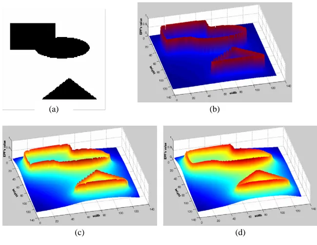
equivalent permittivity. In order to avoid such drawbacks, BEPF is clipped and normalized. Figure 1b-d show the BEPF obtained from a simple binary shape (Figure 1a) for different values of the equivalent background permittivity εeq.

Figure 1. BEPF obtained from a binary image:

(a) original image; (b-d) potential function at εeq = 0.2, 0.05, 0.01, respectively;

2.4 Continuous EPF (CEPF)

Binary EPFs are well suited to binary images, where the edges can be considered simple 2D unit step functions. In the case of gray-level images, the intensity of edges is a source of additional information. In fact, the strength of an edge is usually considered a key parameter to discriminate the significance of a contour point. Then, in order to improve the effectiveness of the matching procedure, the intensity of the edge points is estimated during the edge extraction process by computing the local gradient magnitude, and is retained before binarizing the image. This leads to a variant of the EPF, called continuous EPF (CEPF), computed as follows:

(

)

(

) (

)

∑

where E(xi, yi) is the intensity of the i-th edge point.

It is to be observed that in this case, the intensity of the edge is directly resembled to the charge of the point Qi in the physical model, meaning that a stronger contour attracts to a

(d) (c)

(b) (a)

higher extent a test object. Figure 2c-f show a comparison between BEPF and CEPF calculated from the edge map in Figure 2b extracted from a grey-level image (Figure 2a) for different values of the equivalent background permittivity εeq.

(f) (d)

(a) (b)

(c)

(e)

Figure 2. CEPF obtained from a gray-level image:

(a) original image (256 grey-level); (b) edge map extracted from (a); (c-d) binary potential function at εeq = 0.2, 0.01, respectively; (e-f) continuous potential function at εeq = 0.2, 0.01, respectively.

2.5 Windowed EPF (WEPF)

A major problem common to most edge matching techniques is connected to the presence of clutter and areas with high density of edges, which can lead to a significant rate of false

alarms [31][32]. Multi-resolution approaches have been largely adopted as a strategy to improve both speed and robustness of shape-matching in cluttered environments, as well as to manage partial occlusions and complex transformation parameters. Borgefors [7] proposed to embed a Chamfer matching algorithm into a hierarchical procedure based on a multi-resolution pyramid, to cope with the high number of geometrical transformation parameters requested by the matching procedure. The pyramid is constructed by decreasing at each step the resolution by a factor 4:1 to create the coarser level: the process is iterated until only one pixel is left. Oller et al [41] addressed a similar problem in the edge-based matching of SAR images, where the presence of noise and high-frequency textures makes the problem quite troublesome. In this case the solution consisted in using a variable-size windowing procedure to control the number of pixels in the certain area and reduce the effect of dense edge areas. As far as EPF is concerned, the potential function at each pixel is in principle affected by all the edge points present in the image (see Eq. 3 and 4), although the influence of an edge point rapidly decreases with the distance. Therefore, equivalently to distance transforms EPF may suffer the presence of areas with high edge activity, which locally increase the average potential. CEPF is less sensitive to this problem, for it weights the effect of edges proportionally to their intensity, but may have problems in high contrast areas such as small details or noise.

The solutions to this problem range from the use of sub-sampling and pyramidal approaches, to the use of pre-filtering and/or post-processing tools able to reduce the local edge activity connected to noise and textures, to the introduction of EPF calculation schemes able to limit the impact of dense edge areas on the potential field. In this section, we consider this last approach, achieved through a windowing procedure. Windowed EPF (WEPF) simply consists in defining a window W(εeq) beyond which edge points are ignored. The window is centred

on each image point for which the potential is to be computed, and defines the area within which surrounding edge points have to be considered. A suitable definition of the window size should allow reducing the impact of noise, without altering the concept and effectiveness of EPF. To achieve this result, it is important to consider two aspects: (i) since the windowing procedure results in an approximation of the field, it is desirable that the achieved function is similar to the actual one; (ii) the necessity of reducing the impact of locally dense edge areas on the potential function requires a limitation of the radius of influence relevant to a charged element (a sort of interdiction zone). Remembering that the effect of a charged element on the potential of a given point is in inversely proportional to the distance of the charge itself, we

can conclude that there is a value of the distance (depending also on εeq) after which the

effect of a single charge on the overall potential becomes negligible. The fact of ignoring those charges has a very limited impact on the actual sketch, which is usually a well-defined and linear contour, but can be much more significant in clutter, due to the superposition of effects.

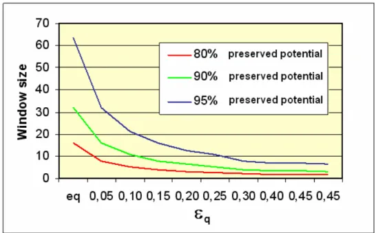
The graph in Figure 3 plots the window size vs. equivalent permittivity, for different percentages of the maximum allowed potential loss for a single charged element (20, 10, 5 percent potential loss, respectively). For instance, if the window size is set according to the lower curve (plotted in red colour), the edge points that contribute to the point potential for less than 20% of their equivalent charge are ignored. In this situation, taking into account that typical values for the equivalent permittivity are in the range [0.02÷0.2], reasonable values for the window size are in the range [6÷15] pixels. Given a constant permittivity, larger losses lead to smaller windows. It has been experimentally proven that a loss of 5% to 10% (i.e., ignoring the edgels that will contribute less than 5-10% of their charge) does not affect at all the precision of the matching, while ensuring a lower computation. This means moving in between the two lower curves in Figure 3.

Figure 3. Window size vs. equivalent permittivity in windowed EPF computation.

It is important to notice that windowing has a positive effect also on the computational complexity. In fact, the computation of the complete potential field will require for each image point a number of floating point operations proportional to the number of edge pixels

present in the image. With WEPF this number becomes proportional to W(εeq), which makes

the method viable also for on-line application.

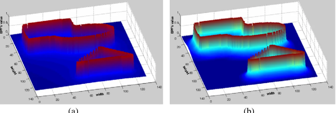
Figure 4 shows the difference between the binary potential function computed using Eq. 3 and one obtained with windowing: it is to be observed that the windowed BEPF is characterized by a larger response near to the contour points and a steeper transition region. Similar results apply to windowed CEPFs.

(a) (b)

Figure 4. Result of approximated computation of BEPF using windows: (a) application to the same image of Fig. 1.a;

(b) difference with exact BEPF (Fig. 1.b)

2.6 EPF-based Similarity Measure

In previous sections, the concept of edge potential function has been defined, as well as some algorithms for its computation. In this section, the application of EPF to shape matching is considered. To this purpose, we define a binary image containing a single shape to be used as a model (sketch image) and a test image in which the model has to be matched (target image).

The first step consists in filtering the target image in order to extract a suitable edge map. Although the optimization of such operation is out the scope of our work, it is important that the extracted edges represent in a robust way the objects present in the scene, irrespectively of the presence of noise and textures. To this purpose, the Canny-Rothwell edge extractor was applied. The EPF of the target image is then calculated. BEPF just requires the edge map, while CEPF uses also the gradient values achieved by the Canny-Rothwell algorithm. The objective of the following process is to determine if the target image contains an object whose shape is similar to the sketch for a given position, rotation and scaling factor. This can be restated as the problem of finding the set of geometrical transformations that maximize the

overlapping between sketch and target, according to a given similarity measure. To this end, the following geometrical operators are taken into account:

™ a rotation, θ;

™ a translation (along the horizontal, t , and vertical, _x t , directions, respectively); _y

™ a scaling (along the horizontal, t , and vertical, _w t , directions, respectively). _h

Horizontal and vertical scaling factors can be constrained to be equal ( ) to keep the aspect ratio constant, thus avoiding deformations. By considering these operators

s h w t t

t = =

(

)

c= , ,θ, , the original sketch is iteratively roto-translated and scaled obtaining different instances of it, which are fitted within the potential field to compute a matching index. The goal is to find the combination of parameters that provides the best fit, and to evaluate if the relevant matching index is high enough to determine with a certain degree of confidence the presence of the model in the target image. As far as the definition of a suitable similarity measure is concerned, the following matching function was defined, namely EPF energy, based on the potential field:

( )

_∑

{

}

n being the n-th pixel of the ck-th instance of the sketch contour, of length pels.

) (c_k

N

f(ck) is therefore the average value of the EPF computed on the target image, calculated along

a curve defined by the current instance of the sketch, and defines the average “attractive energy” generated by the target image upon the roto-translated and scaled version of the sketch. Accordingly, the optimal matching is obtained when the matching function is

maximized, i.e., when the set of transformations is found that provides the maximum average potential along the contour c_opt among all possible transformations.

It is to be pointed out that Eq. 5 does not define a distance function, but rather an average attraction function generated by the edge potential over the model. In other words, in the EP space, point-to-point distances are not measured, but the total (average) attraction energy generated by the target over the model for a given roto-translation and scaling is computed, and the configuration which provides the maximum energy is searched for.

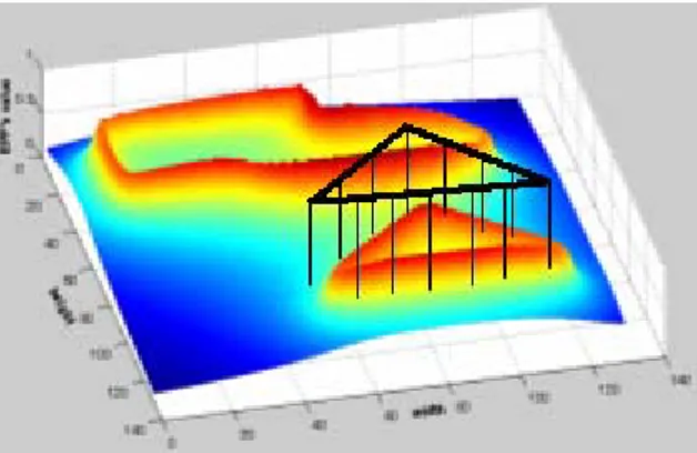
Figure 5 provides a graphical interpretation of the matching process, where the sketch shape is superimposed to the target EPF. The matching function is simply computed by averaging the EPF values at the positions pointed by the sketch pixels.

Figure 5. Computation of the EPF energy

3. EPF and Genetic Algorithms

3.1 Search Strategy and Genetic Algorithms

In section 2, a similarity measure is defined using the concept of Edge Potential. A matching procedure is also outlined consisting in the search of the roto-translation and scaling of the model that maximizes the EPF energy. In this section, the problem of defining a suitable search strategy is addressed. Essentially, the retrieval of the optimal relative position between the sketch and the target is a global optimization problem, where a fitness function should be maximized with respect to a set of parameters that define a geometrical transformation. More specifically, the fitness function proposed in (5) defines a nonlinear multidimensional function, usually characterized by several local maxima. Therefore, the searching strategy should find the global maximum, and avoid remaining trapped in local extremes. Two problems need to be coped with: (i) the large search space and (ii) false matches corresponding to local maxima of the fitness.

Brute-force approaches based on searching all the possible combinations of parameters would lead to unacceptably long processing times, thus being not feasible in practice. On the other side, fast techniques such as gradient descent do not guarantee a good solution, due to the large number of local extremes. Evolutionary approaches are proven to be useful in these situations. Among them, Genetic Algorithms (GAs) are searching processes modelled on the concepts of natural selection and genetics. Their basic principles were first introduced by Holland in 1975 [42] and extended to functional optimization by De Jong [43] and Goldberg [44]. GA is an iterative process in which sets of trial solutions evolve according to pre-defined rules. First, a population of individuals is created randomly, where the population stands for a set of trial solutions, and the individual can be thought of as a candidate solution

and is encoded by a chromosome. The selection is the process by which a new population is

created by making copies of more successful individuals and deleting less successful ones. Throughout this process, crossover and mutation operators are applied with suitable probabilities, to achieve the diversity of individuals. A fitness value is associated to each

individual representing a measure of the solution goodness. The process is stopped whenever an individual is found with the requested fitness, or individuals converge to a stable value. GAs have been recently employed with success in a variety of engineering applications [45][46][47], and in particular in pattern recognition where complex search processes are addressed [48][49][50]. Tsang et al [20] has conducted a thorough research on the use of GAs for object matching under affine invariant transformation condition. Also Kawaguchi et al. exploited the potential of Gas to extract partially occluded objects from a scene, simultaneously detecting rotation, scaling and translation [24][25]. From all of those studies it is clear the one of the most attractive features of GAs is their capability to solve problems involving non-differentiable functions and discrete as well as continuous spaces. Although, these qualities are shared by other multiple-agent procedure techniques, GAs also exhibits an intrinsic parallelism.

In the following section, the use of GAs in combination with EPF is proposed to solve the problem of edge-based visual object detection in digital images.

3.2 Binary GA-based Matching Procedure

The key items in designing a GA-based inversion procedure are: • the representation of the solution, c⇒c~;

• the design of evolutionary operators responsible for the generation of the trial solution succession,

{

}

• the evolutionary procedure.

Different choices result in appropriate procedures able to efficiently deal with different problems. As far as the edge-based detection of visual objects is concerned, a customized binary version of the algorithm has been considered to reduce the computational burden. The objective is to maximize the fitness function (defined in (5)) by finding the optimal set of geometrical transformation parameters, appropriately encoded in the chromosome. To this purpose, a randomly generated population of trial solutions is defined:

{

}

where P is the dimension of the population. Iteratively (being k the iteration number), the

solutions are ranked according to their fitness value

( )

{

}

F_k = _k(p) ; =1,..., =0,..., (7)

and, according to the classical binary-coded version of the GA [47], coded in strings of bits, Li being the number of quantization levels used for the i-th of the 4

unknowns,

{

∑

}

(

)

{

}

Then, new populations of trial solutions are iteratively obtained by applying the genetic operators (selection, crossover and mutation) according to a steady-state strategy [46]. At each iteration, a mating pool is chosen by means of a tournament selection procedure

{ }

k = Γ

Γ _(δ) δ (9)

where δ indicates the selection operator. The new population is generated by applying in a probabilistic way the two-point binary crossover, ξ , and the standard binary mutation, ς

{ }

{ }

The genetic operators are iteratively applied corresponding to their probabilities. Crossover is applied with a probability , mutation is carried out with a probability , and the rest of the individuals are reproduced. The iterative generation process stops when the stationary condition is reached c P P_m conv I i i k k p I f f < −

∑

{

( )

}

= , I is a fixed number of iterations, and is the

convergence threshold.

[

]

As previously specified, the generic solution c=

(

)

(

)

where represent the genes of x-translation, y- translation, rotation, and scaling, respectively. Each gene is coded as a binary string, and must satisfy following conditions: GA s GA GA ty GA tx g g and g g , , _γ , ⎥⎥ ⎤ ⎢⎢ ⎡ ≤ ≤ α w g_txGA 0 , ⎥⎥ ⎤ ⎢⎢ ⎡ ≤ ≤ α h gtyGA 0 , ⎥ ⎥ ⎤ ⎢ ⎢ ⎡ − ≤ ≤ β min max 0 g_sGA R R , ⎥ ⎥ ⎤ ⎢ ⎢ ⎡ − ≤ ≤ γ min max 0 gGA S S s (13)

where α ,β and γ are the relevant steps for discrete translation, rotation, and scaling; w, h, , , , and are the width and height of the target image, the lowest and highest rotation angles and the lowest and highest scaling bounds, respectively.

min

R R_max S_min S_max

Consequently, the total number of bits of the chromosome turns out to be: ⎥ ⎥ ⎤ ⎢ ⎢ ⎡ − + ⎥ ⎥ ⎤ ⎢ ⎢ ⎡ − + ⎥⎥ ⎤ ⎢⎢ ⎡ + ⎥⎥ ⎤ ⎢⎢ ⎡ = γ β α α 2 max min min max 2 2

2 log log log

log w h R R S S

N (14)

4. Experimental Results

The proposed technique has been extensively tested in several experimental configurations and different data sets. In this section we summarize the results of this analysis, focusing on three aspects: (i) to assess the potential of EPF as a similarity measure in itself; (ii) to evaluate the performance of EPF-based matching methods using GAs as a searching strategy; (iii) to assess the performance of EPF-based matching in extremely critical situations, where the analyzed data are affected by serious noise and clutter conditions. These aspects are subsequently treated in the following three sections. For all the presented test cases, a comparison with highly optimized implementations of competing edge-based matching techniques is proposed.

In order to comparatively assess the effectiveness of the proposed approach with respect to competing state-of-art techniques, three representative examples are analyzed. The first refers to a synthetic image without noise, but containing several objects with similar shape. The second is a much more complex and cluttered image with high density of contours. The last one is a natural color image characterized by complex and repetitive shapes with weak edges. As far as the compared techniques are concerned, they are denoted as follows:

• CM: Chamfer Matching • HD: Hausdorff Distance

• WEPF: Windowed EPF (window size = 32 pels, permittivity ε = 0.02)

Since we are interested in comparing the similarity measures unaffected by the matching procedure, in these examples a full-search strategy has been applied, by computing the similarity index of the three methods for every possible parameters configuration. The following TABLE 1 provides the variation range of each parameter.

TABLE 1.RANGE OF PARAMETERS FOR FULL SEARCH PROCEDURE

Transform operator Range Step

Translation X [0, w=image width] α = 2 Translation Y [0, w=image height] α = 2 Rotation Rmin=1, Rmax=360 β = 3 Scaling Smin=0.7, Smax=1.3 γ = 0.1

The number of quantization levels has a direct impact on the accuracy of the matching. For instance, if the translation step is set to 5 pixels, a maximum displacement of 2 pixels is expected. This condition limits a lot the choice of quantization steps. Moreover, the precision on translation has to be correlated to the precision on scaling and rotation. As a matter of fact, it would be useless to have a maximum error of 1 pixel in translation and a maximum error of 5 or more pixels due to the rotation or translation (this also depends on the size of the object). In this sense, the parameters defined in TABLE 1 were carefully selected, also taking into account the resolution of images and size of searched objects.

In Figure 6a-b the first image and the relevant query are shown.

Figure 6. A synthetic test image (a) Target image, (b) Query image

In Figure 7 the histogram of the similarity values calculated with the three techniques are reported. As it can be observed, the EPF-based similarity is the only one that shows a sharp decrease of the number of samples in correspondence with the larger fitness values. In particular, only for windowed EPF the maximum fitness (equal to 1) is associated to the optimal solution only (i.e., the perfect overlapping between the query and the target image).

(a) (b)

(c)

Figure 7. Histogram of the similarity values relevant to the image in Figure 6: (a) HD, (b) CM, and (c) WEPF

In

Figure 8 and Figure 10 the other two examples are depicted. In both cases, the edge map is extracted from the greyscale/colour image by a Canny-Rothwell edge detector with σ = 1.5. The relevant similarity histograms are proposed in Figure 9 and Figure 11, respectively, using the same sets of parameters. The behavior is clearly analogous to the one previously discussed.

(a) (b)

(c) (d)

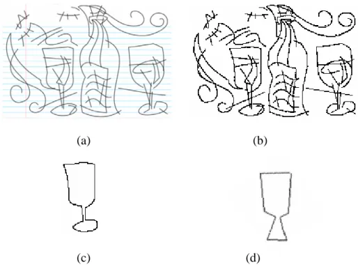
Figure 8. A greyscale test image showing several hand-draw objects

(a) Original image (b) relevant edge map (c) query image extracted from the test image (d) query image drawn by user.

(a) (b)

Figure 9. Histogram of the similarity values relevant to the image in Figure 8:

(a) HD, (b) CM, and (c) WEPF

(a) (b) (c)

Figure 10. Colour test image

(a) Original image (b) relevant edge image (c) query image

(a) (b)

(c)

Figure 11. Histogram of the similarity values relevant to the image in Figure 10: (a) HD, (b) CM, and (c) WEPF

The curves in Fig. 7, 9, 11 demonstrate that the proposed algorithm generates a lower number of “highest-score” points. This is a positive feature, provided that these points correspond to the correct positioning of the object. On the other hand, HD and CM tend to have a large

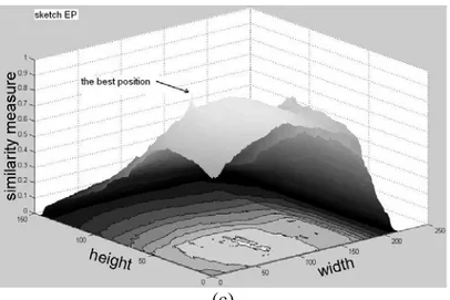
number of positions with very high score. This behavior of HD and CM is not necessarily negative, provided that the relevant positions are concentrated in the correct position. It is then necessary to study the distribution of the peaks of the fitness function in the different cases. The following Figs. 12, 13 show the behavior of the fitness function for the three methods along all the possible x,y translations, keeping constant rotation and scaling. It is possible to observe that with EPF the points with higher scores form a slope around the solution, with a unique peak, while the numerous “high-match” points achieved by the other two methods are in fact spread over the image and not concentrated near the correct solution. This fact demonstrates that EPF eases the optimization process, making it possible to detect the correct matching.

(a)

(c)

Figure 12. 3D surface of the similarity values relevant to the image in Figure 6: (a) HD, (b) CM, and (c) WEPF

(a)

(c)

Figure 13. 3D surface of the similarity values relevant to the image in Figure 10: (a) HD, (b) CM, and (c) WEPF

4.2. Edge matching procedure using EPF and GAs

In this section, EPF is compared with other methods in terms of matching capabilities. In order to avoid the dependence of the result on the searching strategy, the same optimized GA searching procedure has been applied. In Figure 14, the dialog box specifying the GA parameters is shown.

It should be noted that the position of the sketch in the model image has no effect at all on the matching procedure. In fact, the initial population is randomly generated applying casual roto-translation and scaling to that shape. Then, the probability of having the exact instance of the model which corresponds to the target object in the initial population is exactly the same of any other transformation.

The following Figure 15-16 depict, for each of the three selected test cases described in Sect. 4.1, the behavior of the fitness function during the iterative process, and the best matching achieved at convergence.

Figure 14. GA parameters setting

(c) (d)

(e) (f)

Figure 15. Result of matching on the image in Figure 6.

Left column: behaviour of the fitness function; Right column: best matching. First row: HD, Second row: CM, Third row: WEPF

(c) (d)

(e) (f)

Figure 16. Result of matching on the image in Figure 8 with the query is

Figure 8c.

Left column: behaviour of the fitness function; Right column: best matching. First row: HD, Second row: CM, Third row: WEPF

(a) (b)

(c) (d)

(e) (f)

Figure 17. Result of matching on the image in Figure 8 with the query is

Figure 8d.

Left column: behaviour of the fitness function; Right column: best matching. First row: HD, Second row: CM, Third row: WEPF

(a) (b)

(c) (d)

(e) (f)

Figure 18. Result of matching on the image in Figure 10.

Left column: behaviour of the fitness function; Right column: best matching. First row: HD, Second row: CM, Third row: WEPF

Looking at the matching results, it can be observed that WEPF performance is extremely satisfactory, for the correct shape is located in all examples. In the first test, HD and CM converge to a local maximum in correspondence with a similar shape in the bottom-left of the image. Also WEPF does not achieve a perfect matching, although it converges to the right object location. In the other two examples, WEPF achieves almost perfect matching, while other approaches are attracted by high-density edge areas, thus not converging to a reasonable solution.

It should be noted that EPF tends to give lower fitness values as compared to other techniques. This is evident looking at the 3D charts of the potential (Figure 1), which show how the potential decreases quite rapidly. Nevertheless, this is not a negative characteristic of

the method. In fact, what is really important here is the relative value of the fitness and not the absolute one. As seen in above examples, HD or CM can produce a wrong solution with a high fitness, then, the result may be not reliable even if the score is very high. On the other side, EPF provides the correct position, associated to the highest score, even if the relevant absolute value may not be close to 1 due to imperfect overlapping with the model (e.g., due to quantization step or differences between model and target).

Fig. 17 shows the result achieved by applying the human-drawn query of Fig. 8.d. In that case, the model is similar but not identical to the target. The test demonstrates that also in this situation EPF achieves a very good matching.

The last example of this section deals with a possible application to image indexing and retrieval based on visual object matching. In this case, we imagine that a user can browse an image database by sketching a shape on a simple graphical interface. The relevant contours are then matched with the images in the database, in order to detect similar objects. In the proposed example, the database was made up of more than 400 color pictures of monuments, town views, landscapes and other subjects.

In Figure 19a a sketch query is represented, while in Figure 19b, the precision-recall curve achieved by the EPF-based indexing is compared to those of HD and CM. Precision-recall curve is a very common measure to evaluate the performance of a information retrieval process. Assuming that:

- RET = set of all images the system has retrieved for a specific query; - REL = set of relevant images in the database for the query;

- RETREL = set of the relevant images retrieved by the algorithm; then, precision and recall measures are obtained as follows:

- precision = RETREL / RET - recall = RETREL / REL

For the sake of completeness, Fig. 16c reports the set of most relevant samples extracted from the database with the proposed approach. In each image, the best match is superimposed in white. It can be observed that the achieved ranking is very good. As an example, let us consider that the subset of Eiffel tower images is composed of 19 images, which are successfully retrieved among the first 26 ranked samples.

(a) (b)

(c)

Figure 19. Use of WEPF for image indexing and retrieval.

(a) a user sketch used for query; (b) comparative precision-recall diagram; (c) retrieval result.

One of the key advantages of EPF-based matching is the capability of making coherent contours prevail over noise spots. In order to experimentally assess this feature of the proposed method, a further set of tests is presented in this section, in which the matching is performed in extremely critical noise conditions. The first test case refers to the “flowers” image (Figure 10a). It consists in performing the matching in the presence of a high-power additive Gaussian noise. The noisy image and the relevant query are presented in Figure 20a-b, while Figure 20c depicts the edge map extracted by the Canny-Rothwell algorithm, showing a strongly damaged edge map (contours fragmentation, noise spots). In Figure 20d-f the results of the matching are presented, again comparing the proposed methods with the optimized HD and CM techniques. As expected, the accuracy of WEPF in locating the right shape turns out to be slightly reduced (see Figure 20f vs. Figure 18f). Nevertheless, it should be noticed that WEPF definitely outperforms other methods.

(a) (b) (c)

(d) (e) (f)

Figure 20. Matching results in the presence of high-power Gaussian noise:

(a) noisy target image, (b) relevant edge map, (c) query, (d) HD, (e) CM, (f) WEPF

In the second test case, a high-frequency texture is added to the same “flowers” image (Figure 10a). The texture strongly distorts the image, thus producing a cluttered edge map

(Figure 21c). In Figure 21d-f the results of the matching of the query (Figure 21b) are presented, again comparing the proposed methods with the optimized HD and CM techniques. Also in this case, WEPF is the only method to achieve a correct matching.

(a) (b) (c)

(d) (e) (f)

Figure 21. Matching results in the presence of texture noise: (a) noisy target image, (b) relevant edge map, (c) query,

(d) HD, (e) CM, (f) WEPF

Finally, the third example concerns the detection of a simple triangular object. Here, the main difficult is in the fact that the target shape is strongly fragmented (a dashed line) and it is immersed in a high-frequency texture. The test image and the query are shown in Figure 22a-b, while the matching results for the three competing techniques are depicted in Figure 22c-e. Again, it is possible to observe that only the EPF-based approach converges to the correct solution, while HD and CM are mislead by the highly dense edge map generated by the background texture.

(a) (b)

(c) (d) (e)

Figure 22. Matching results in the presence of high-frequency background texture:

(a) target image, (b) query,(c) HD, (d) CM, (e) WEPF

The interpretation of these last results is that in most complex situations, where edges are weak and noise or textures tend to prevail, it is very important the property of EPF of exploiting the superposition of effects between edge points along the target curve, so that coherent structures acquire a greater weight in the fitness function.

4.3. Algorithm convergence and complexity issues

Studies have been carried out in order to ascertain the convergence properties of the proposed algorithm and its computational complexity. As far as the verification of the convergence of the GA is concerned, due to the stochastic nature of the algorithm the figures reported throughout the paper refer to average values achieved by multiple runs of the algorithm (10 executions for each test, with randomly generated initial populations).

In order to show the steadiness of the algorithm, in Table 3 we report the complete test set for the example of Fig. 17. Each row shows the result of the run in terms of best fitness and resulting affine transform parameter set.

TABLE 2.STATISTICAL REPORT OF EXAMPLE IN FIGURE 17

Bold rows denote the best match under human perspective

Times Fitness at

convergence

1 0.895831 (53, 53, 1, 0) 2 0.906262 (52, 54, 1, 0) 3 0.890051 (49, 62, 1, 6) 4 0.884643 (51, 56, 1, 3) 5 0.869046 (61, 53, 0.9, 0) 6 0.895985 (52, 55, 1, 0) 7 0.878611 (49, 49, 1, 6) 8 0.903584 (50, 58, 1, 3) 9 0.894045 (59, 53, 1, 356) WEPF 10 0.87052 (51, 62, 0.9, 3) 1 0.994031 (108, 60, 0.9, 303) 2 0.994437 (133, 73, 0.9, 273) 3 0.995021 (134, 104, 0.9, 263) 4 0.995937 (134, 98, 0.9, 267) 5 0.995496 (114, 127, 0.9, 189) 6 0.994713 (47, 101, 0.9, 65) 7 0.993689 (55, 45, 0.9, 353) 8 0.995937 (134, 98, 0.9, 267) 9 0.994646 (53, 107, 0.9, 75) CM 10 0.994377 (154, 88, 0.9, 189) 7 1 0.995928 (134, 98, 0.9, 267) 2 0.994132 (61, 55, 0.9, 6) 3 0.994389 (195, 72, 0.9, 276) 4 0.993919 (48, 39, 0.9, 6) 5 0.994667 (117, 125, 0.9, 192) 6 0.994192 (60, 68, 0.9, 12) 7 0.995737 (133, 96, 0.9, 270) 8 0.995508 (135, 98, 0.9, 267) 9 0.994121 (125, 82, 0.9, 281) HD 10 0.994132 (155, 92, 0.9, 189)

It is possible to observe that in EPF the best match between the query and the target image under human perspective has the highest fitness at convergence. On the contrary, for CM and HD the best match under human perspective does not correspond to the highest fitness. This demonstrates that EPF works well in complex environments, where CM and HD tend to remain trapped in local maxima.

As far as the computational complexity is concerned, it is to be pointed out that the proposed approach implies a higher cost for the calculation of the potential function, while it is characterized by an almost equivalent cost for the computation of the fitness function, used in the optimization process. This drawback turns out to be acceptable in many applications (e.g., image indexing and retrieval applications), where the computation of the EPF can be performed off-line and stored for each target image, thus not affecting the matching time. In the case of on-line computation of the EPF, the overall matching time slightly increases. The following TABLE 3 indicates the CPU time relevant to the above examples when different methodologies are used. The reported times (in seconds) refer to the execution of the code on PC equipped with a P4 processor at 2.6GHz. It can be noticed that the computation of the EPF matrix is higher as compared to nearest-neighbor-based approaches, while GAs convergence requires similar CPU time. Moreover, the computation of the EPF is strongly dependent on the complexity of the edge image (since the number of “equivalent charges” to be considered increases with the edge density), and of course it benefits of the windowing procedure.

TABLE 3. COMPARISON IN TERMS OF COMPUTATION TIME (IN SECONDS) Bottle (216 x 146) Flower (144 x 160) Synthetic (114 x 96) Time to run GA Time to compute EP/CF Time to run GA Time to compute EP/CF Time to run GA Time to compute EP/CF EPF 5.047 13.609 2.469 2.968 2.984 0.719 WEPF 32 5.031 11.75 2.485 2.968 2.984 0.703 WEPF 16 5.069 10.03 2.481 2.468 2.75 0.578 CM 5.187 0.453 2.468 0.281 2.891 0.156 HD 5.375 0.453 2.5 0.281 2.984 0.156

A further note concerns the dependence of the GA convergence on the number of quantization levels used in the encoding of the parameters. This is a not trivial task, since the best performance of the optimizer occurs when a good trade-off between exploration of the searching space and exploitation of the best features of trial solutions is achieved. As a matter of fact, a coarse quantization does not require large populations, but it does not allow achieving a satisfactory matching, due to the granularity of the geometrical transformations. On the other hand, a finer quantization can achieve a closer matching, while significantly enlarging the solution space, thus requiring a larger population in order to converge in a reduced number of iterations.

5. Conclusions

A new approach to the problem of edge-based visual object matching in digital images was presented, based on the concept of Edge Potential Function (EPF) and the use of a GA-based optimization. The potential function is calculated starting from the edge map of the image, and it is used as an attraction pattern in order to find the best possible match with a template or hand-drawn sketch.

Different possible approaches to the computation of the EPF were suggested, including binary and continuous functions, as well as windowed procedures. The new approach was extensively tested on both synthetic and photographic pictures, showing very good performance in comparison with state-of-the-art methods. It is worth noting that, thanks to the capability of exploiting the joint effect of continuous charges aligned over coherent structures, EPF matching demonstrated a reliable performance also in the presence of high-power noise and clutter. Furthermore, it is effective also when the sketch does not fit exactly the target image, thus allowing the development of effective and robust tools in the framework of content-based image retrieval applications.

Future developments will take into consideration additional features of the potential field not exploited in the present implementation, such as the direction and continuity information.

6. Acknowledgements

This work has been partially funded by the Italian Ministry under the framework of the FIRB programme (project VICOM).

7. References

[1] R.C. Veltkamp and M. Hagedoorn, “State-of-the-Art in Shape Matching,” Principles of visual information retrieval, Springer-Verlag, London, UK, ISBN:1-85233-381-2, pp. 87-119, 2000. [2] V.N. Gudivada, and V.V. Raghavan, “Content-Based Image Retrieval Systems,” Computer,

Vol. 28, No. 9, pp. 18-21, Sept. 1995.

[3] S.F. Chang, “Content-Based Indexing and Retrieval of Visual Information,” IEEE Signal Processing Magazine, pp. 45-48, July 1997.

[4] A.W.M. Smeulders, M. Worring, S. Santini, A. Gupta, R. Jain: “Content-based image Retrieval at the End of the Early Years”. IEEE Transactions on Pattern Analysis and Machine

Intelligence, Vol. 22, No.12, pp. 1349-1380, Dec. 2000.

[5] I. Biederman, “Human image understanding: Recent research and a theory,” Computer Vision, Graphics, and Image Processing, vol. 32, pp. 29-73, 1985.

[6] M.I. Posner, “Foundations of cognitive Science,” Editor MIT Press, ISBN: 0262161125, 1989. [7] G. Borgefors, “Hierarchical Chamfer Matching: A Parametric Edge Matching Algorithm”,

IEEE Trans. on Pattern Analysis and Matching Intelligence, Vol. 10, No. 6, pp. 849-865, Nov. 1988.

[8] S. Loncaric, “A Survey of Shape Analysis Techniques,” Pattern Recognition, vol. 31, no. 8, pp. 983-1001, 1998.

[9] D. G. Kendall, D. Barden, T.K. Carne, and H. Le, Shape and Shape Theory. Wiley, Chichester, England, 1999.

[10] F.L. Bookstein, “Size and shape spaces for landmark data in two dimensions,” Statistical Science, vol. 1, no. 2, pp. 181-242, 1986.

[11] I. Dryden and K. Mardia, Statistical Shape Analysis. New York: Wiley, 1998.

[12] I. Dryden, “Statistical shape analysis in high-level vision”, in Proc. of IMA workshop on Image Analysis and High Level Vision Modelling, 2000.

[13] T. Cootes, C. Taylor, D. Cooper, and J. Graham, “Active shape models – their training and application,” Computer Vision and Image Understanding, vol. 61, no. 1, pp. 38-59, 1995. [14] T.K. Carne, “The geometry of shape spaces,” Proc. of the London Mathematic Society, vol. 3,

no. 61, pp. 407-432, 1990.

[15] C.G. Small, The Statistical Theory of Shape, Springer, 1996.

[16] N. Naswani, A.R. Chowdhury, and E. Chellappa, “Statistical Shape Theory for Activity Modelling”, In Proc. of ICASSP 03.

[17] U. Grenander, General Pattern Theory, Oxford University Press, England, 1993. [18] A. Srivastava, S.H. Joshi, W. Mio, and X. Liu, “Statistical Shape Analysis: Clustering,

Learning, and Testing,” IEEE Trans. on Pattern Analysis and Machine Intelligence, vol. 27, no. 4, April 2005.

[19] F. Mokhtarian, “Silhouette-Based Isolated Object Recognition through Curvature Scale Space,” IEEE Trans. on Pattern Analysis and Machine Intelligence, vol. 17, no. 5, pp. 539-544, May 1995.

[20] P.W.M. Tsang, “Enhancement of a Genetic Algorithm for Affine Invariant planar Object Shape Matching Using the Migrant Principle,” IEEE Image and Signal Processing, vol. 150, no. 2, pp. 107-113, 2003.

[21] G. L. Scott and H. C. Longuet-Higgins, "An Algorithm for Associating the Features of Two Patterns," Proc.of the Royal Society B, B244, pp. 21-26, 1991.

[22] Y. Xu, E. Saber, and A.M. Tekalp, “Image Retrieval through Shape Matching of Partially Occluded Objects Using Hierarchical Content Description,” Proc. International Conference on Image Processing, pp. 73-76, 2000.

[23] J.R. Beveridge, H. Weiss, E.M. Riseman, “Combinatorial Optimization Applied to Variable Scale 2D Model Matching,” Proc. 10th International Conference on IEEE Pattern Recognition, pp. 18-23, 1990.

[24] T. Kawaguchi, R.I. Nagata, and T. Sinozaki, “Detection of Target Models in 2D Images by Line-Based Matching and a Genetic Algorithm,” Proc. International Conf. on IEEE Image Processing, vol. 2, pp. 710-714, 1999.

[25] T. Kawaguchi and M. Nagao, “Recognition of Occluded Objects by a Genetic Algorithm”,

Proc. 14th International Conf. on IEEE Pattern Recognition, vol.1, pp. 233-237, 1998.

[26] H.G. Barrow, J.M. Tenenbaum, R.C. Bolles, and H.C Wolf, “Parametric correspondence and Chamfer matching: Two new techniques for image matching”, Proc. 5th Int. Joint Conf. Artificial Intelligence, Cambridge, MA, pp. 659-663, 1977.

[27] E. Akleman and J. Chen, “Generalized Distance Functions,” Proc. Shape Modeling International Conf. on Shape Modeling and Applications, pp. 72-79, 1999.

[28] G. Borgefors, “Distance transformations in Digital Image,” Computer Vision, Graphics, and Image Processing, vol.34, pp. 344-371, 1986.

[29] D.P. Huttenlocher, G.A. Klanderman, and W.J. Rucklidge, “Comparing Images Using the Hausdorff Distance,” IEEE Trans. on Pattern Analysis and Machine Intelligence, vol.15, no.9, pp. 850-863, Sep. 1993.

[30] D.P. Huttenlocher and W.J. Rucklidge, “A Multi-Resolution Technique for Comparing Images Using the Hausdorff Distance,” Proc. International Symposium on Computer Vision, pp. 705-706, 1993.

[31] C.F. Olson and D.P. Huttenlocher, “Recognition by Matching Dense, Oriented Edge Pixels,” Proc. International Symposium on Computer Vision, pp. 91-96, 1995

[32] C.F. Olson and D.P. Huttenlocher, “Automatic Target Recognition by Matching Oriented Edge Pixels,” IEEE Trans. on Image Processing, vol.6, no.1, pp. 103-113, January 1997.

[33] D.G. Sim and R.H. Park, “Two-Dimensional Object Alignment Based on the Robust Oriented Hausdorff Similarity Measure,” IEEE Trans. on Image Processing, Vol. 10, No. 2, pp. 475-483, 2001.

[34] B. Li, Q. Meng, and H. Holstein, “Point Pattern Matching and Applications – a Review,” IEEE, vol., no., pp. 729-736, 2003.

[35] J. Wang, K.W. Bowyer, T.A. Sanocki, and S. Sarkar, “The Effect of Edge Strength on Object Recognition from Edge Images,” Proc. International Conference on Image (ICIP 98), pp. 45-49, 1998.

[36] M.I. Chowdhury and J.A. Robinson, “Improving image segmentation using edge information,” Proc. Conference on Electrical and Computer Engineering, vol. 1, pp. 312-316, 2000.

[37] W.Y. Ma and B.S. Manjunath, “EdgeFlow: A Technique for Boundary Detection and Image Segmentation,” IEEE Trans. in Image Processing, vol. 9, no. 8, pp. 1375-1388, 2000 [38] C.F. Olson, “Maximum-Likelihood Image Matching,” IEEE Trans. on Pattern Analysis and

Machine Intelligence, vol. 24, no. 6, pp. 853-857, 2002.

[39] O. Khatib, “Real-time Obstacle Avoidance for Manipulators and Mobile Robots,” The International Journal of Robotics Research, vol. 5, no. 1, pp. 90-98, 1986.

[40] J.A. Stratton, Electromagnetic Theory. McGraw-Hill Book, NY 1941.

[41] G. Oller, P. Marthon, and L. Denise, “SAR image matching using the edge strength map,” Proc. IEEE International Conference on Geoscience and Remote Sensing Symposium (IGARSS '02), vol. 4 , pp. 2495-2497, 2002.

[42] J.H. Holland, “Adaptation in Natural and Artificial Systems”, Univ. Michigan Press, Ann Arbor, 1975.

[43] K.A. De Jong, “An analysis of the behavior of a class of genetic adaptive systems”, Ph. D. Dissertation, Univ. Michigan, 1975.

[44] D.E. Goldberg, Genetic Algorithms in Search, Optimization and Machine Learning. Reading, MA: Addison-Weiley., 1989.

[45] J. Inglada and F. Adragna, “Automatic multi-sensor image registration by edge matching using genetic algorithms,” Proceedings of International Conference on Geoscience and Remote Sensing Symposium (IGARSS'01), vol. 5, pp. 2313 – 2315, 2001

[46] J.M. Johnson and Y.R. Samii, “Genetic Algorithms in engineering electromagnetics,” IEEE Trans. on Antennas and Progat. Magazine, vol. 39, no. 4, pp. 7-25, August 1997.

[47] M. Pastorino, A. Massa and S. Caorsi, "A microwave inverse scattering technique for image reconstruction based on a genetic algorithm," IEEE Transactions on Instrumentation and Measurement, vol. 49, no. 3, pp. 573-578, June 2000.

[48] Y.K., Wang and K.C. Fan, “Applying Genetic Algorithm on Pattern Recognition: An Analysis and Survey,” Proceedings of ICPR’96, pp. 740-744. 1996.

[49] L. Zhang, W. Xu, and C. Chang, “Genetic algorithm for affine point pattern matching,” Pattern Recognition Letters, vol. 24, pp. 9-19, 2003.

[50] P.Y. Yin, “A new circle/ellipse detector using genetic algorithms,” Pattern Recognition Letters, vol. 20, pp. 731-740, 1999.