A Dissimilarity based on Relevant Population
Features
M. Cubedo, A. Mi˜narro and J.M. Oller∗ Departament d’Estad´ıstica
Universitat de Barcelona 08028 Barcelona, Spain
May 16, 2012
∗This work is partially sponsored by MTM 2008–00642 (Ministerio de Ciencia e Innovaci´on),
Abstract
In this paper a dissimilarity index between statistical populations is pro-posed without the hypothesis of a specific statistical model. We assume that the studied populations differ on some relevant features which are measured trough convenient parameters of interest. We assume also that we dispose of adequate estimators for these parameters. To measure the differences be-tween populations with respect the parameters of interest, we construct an index inspired on some properties of the information metric which are also presented. Additionally, we consider several examples and compare the ob-tained dissimilarity index with some other distances, like Mahalanobis or Siegel distances.
Keywords and phrases: Information metric, Mahalanobis distance, Siegel distance, Dissimilarity index.
1 Introduction
The distance concept has been proved to be a very useful tool in data analysis and statistics, in order to study the similarity or dissimilarity between physical objects, usually, in a wide sense, populations. See for instance the classical works of Mahalanobis (1936), Bhattacharyya (1942) or Rao (1945), the foundations of the information metric studied in Atkinson and Mitchell, Burbea and Rao (1982), or Burbea (1986), some applications to statistical inference in Amari (1985), Oller and Corcuera (1995) or Cubedo and Oller (2002), applications to data analysis in Gabriel (1971), Huber (1985), Friedman (1987), Gower and Harding (1988), Greenacre(1993), Cook, Buja, Cabrera, and Hurley (1995) or Gower and Hand (1996) and more recent papers on foundations of distances in statistics like Lindsay, Markatou, Ray, Yang and Chen (2008) among many others.
In the present paper we are interested to define a distance between p different statistical populations Ω1, · · · , Ωp. We assume that the studied populations
dif-fer on some relevant features which are measured trough convenient parameters of interest ξ = (ξ1, · · · , ξk)t, although we shall not suppose a particular
paramet-ric statistical model for the distribution of data. After obtaining for every statistical population a data matrix Xiof order ni×m, we define certain convenient vectorial
statistic T = (T1, . . . , Tk)t, and we assume that it is an unbiased and consistent
estimator of ξ in each population. From this relevant statistic T we shall construct a dissimilarity index between statistical populations, which we shall refer hereafter as Relevant Features Dissimilarity (RFD). This index is inspired on some proper-ties of the information metric. Additionally, a Multidimensional Scaling has been
realized to compare the differences between our dissimilarity with Mahalanobis and Siegel distances.
2 Some remarks on the information metric
We first introduce some notation. Let χ be a sample space,
a
a σ–algebra of subsets of χ and µ a positive measure on the measurable space (χ,a
). In the present paper, a parametric statistical model is defined as the triple {(χ,a, µ) , Θ , f }, where
(χ,a
, µ) is a measure space, Θ, also called the parameter space, is a manifold, and f is a measurable map, f : χ×Θ −→ R such that f (x, θ) ≥ 0 and dPθ = f (·, θ)dµ is a probability measure on (χ,a
), ∀θ ∈ Θ. We shall refer µ as the referencemeasure of the model.
Although in general Θ can be any manifold, for many purposes it will be enough to consider the case that Θ is a connected open set of Rn, and, in this case, it is customary to use the same symbol (θ) to denote points and coordinates, notation which we are going to use hereafter. Additionally, we shall assume that function f satisfy certain standard regularity conditions which allow us to define on Θ a Riemannian structure induced by the probability measures, referred as the
information metric, and given by ds2=
n
X
i,j=1
gij(θ)dθidθj
where gij(θ) are the components of the Fisher information matrix. For further
details, see Amari (1985), Atkinson and Mitchell (1981), Burbea and Rao (1982) or Burbea (1986) among many others.
Let us denote the expectation, the covariance and the variance, with respect the probability measure dPθ = f (·, θ)dµ, as Eθ(X), covθ(X, Y ) and varθ(X) respectively.
Let us define now D as the class of maps X : χ × Θ −→ R such that X(·, θ) is measurable map with finite variance with respect the probability measure dPθ, ∀θ ∈ Θ, which additionally satisfy the condition
∂ ∂θi Eθ(X(·, θ)) = Z χX(x, θ) ∂f (x, θ) ∂θi dµ, ∀θ ∈ Θ, i = 1, . . . , n
Observe that this condition is fulfilled in many situations, for instance when X is not dependent on θ or in most of the cases when Eθ(∂X(·, θ)/∂θi) = 0, like X(x, θ) = log f (x, θ).
Additionally, let us consider the n-dimensional vector space: Hθ = < ∂ log f (·, θ) ∂θ1 , . . . , ∂ log f (·, θ) ∂θn > ⊂ L 2(f (·, θ) dµ)
where we have identified, as usual, the functions ∂ log f (·, θ)/∂θi, which form a
basis of Hθ, as elements of L2(f (·, θ) dµ). Then Hθ inherits a scalar product, <, >Hθ= covθ(·, ·), since Eθ(∂ log f (·, θ)/∂θi) = 0. Observe that, with respect
the above-mentioned basis, the corresponding scalar product matrix is the Fisher information matrix G = (gij(θ)).
We can identify this Euclidean vector space with the tangent space at θ, Θθ, which also has an Euclidean structure induced by the information metric, through the correspondence: n X k=1 Zk ∂ log f (·, θ) ∂θk ←→ n X k=1 Zk µ ∂ ∂θk 
which is, clearly, a natural lineal isometry between Hθ and Θθ. Then, fixed θ, the
tangent vectors may be viewed as random maps, and we shall make use of this identification, hereafter, when necessary.
Notice also that the projection map πθ : L2(f (·, θ) dµ) −→ H
θis well defined,
with X(·, θ) − πθ(X(·, θ)) ∈ Hθ⊥. The following proposition make explicit some
properties of the above–mentioned identification.
Proposition 2.1 Let X ∈ D and define U (·, θ) = πθ(X(·, θ)) and V (·, θ) = X(·, θ) − U (·, θ). Then a) U (·, θ) = n X i=1 Xn j=1 gij(θ) covθ µ X(·, θ),∂ log f (·, θ) ∂θj ¶ ∂ log f (·, θ) ∂θi
where gij(θ) are the elements of the inverse of the Fisher information matrix,
G = (gij(θ)).
Moreover, identifying the tangent vectors with the elements of Hθ, we have
b) grad (Eθ(X(·, θ))) = U (·, θ) c) kgrad (Eθ(X(·, θ))) k2
θ = varθ(U (·, θ)) d) varθ(X(·, θ)) = kgrad (Eθ(X(·, θ))) k2
Proof:
Observe that U (·, θ) = πθ(X(·, θ)) ∈ Hθ then
U (·, θ) = U1∂ log f (·, θ)
∂θ1 + . . . + Un
∂ log f (·, θ) ∂θn
where the coefficients Uiare determined in order to minimize kX(·, θ)−U (·, θ)k2 θ.
It is straightforward to prove that
(1) Ui = n X j=1 gij(θ) covθ µ X(·, θ),∂ log f (·, θ) ∂θj 
and a) follows. On the other hand, since X ∈ D and thusEθ
µ ∂ log f (·, θ) ∂θi ¶ = 0, we have ∂ ∂θi Eθ(X(·, θ)) = Z χX(x, θ) ∂f (x, θ) ∂θi µ(dx) = covθ µ X(·, θ),∂ log f (·, θ) ∂θi 
Therefore the i-th component of grad (Eθ(X(·, θ))), with respect the basis vector field ∂/∂θ1, . . . ∂/∂θn, at θ, is given by grad (Eθ(X(·, θ)))i = n X α=1 giα(θ) covθ µ U (·, θ),∂ log f (·, θ) ∂θα 
and taking into account (1) and the natural lineal isometry between Hθand Θθ, we can write
grad (Eθ(X(·, θ))) = U (·, θ)
the square of its norm is given by
kgrad (Eθ(X(·, θ))) k2
θ = varθ(U (·, θ))
and since X(·, θ) = U (·, θ) + V (·, θ) and covθ(U (·, θ), V (·, θ)) = 0 we obtain
varθ(X(·, θ)) = kgrad (Eθ(X(·, θ))) k2
θ+ varθ(V (·, θ))
completing the proof. ¥
Let us define now S ⊂ D as the subclass of maps such that varθ(X(·, θ)) ≤ 1
∀θ ∈ Θ, then from Proposition 2.1, as an immediate consequence, we have the
Corollary 2.2 Let X ∈ S then
kgrad (Eθ(X(·, θ))) kθ≤ 1 ∀θ ∈ Θ
We can prove also the following property
Proposition 2.3 Let X ∈ D, and let α : [a, b] −→ Θ be a piecewise C∞curve parametrized by the arc length, a, b ∈ R, a < b, such that ν = α(a) and ξ = α(b). Let also define ΦX(θ) = Eθ(X(·, θ)) and ∆ΦX = ΦX(ξ) − ΦX(ν).
Then (2) ¯ ¯ ¯ ¯d(ΦXds◦ α) ¯ ¯ s=s∗ ¯ ¯ ¯ ¯ ≤ σX(α(s∗)) and (3) |∆ΦX| ≤ µ max s∈[a,b]σX(α(s)) ¶ l(ν, ξ) where l(ξ, ν) is the curve length between ν and ξ, and σX(θ) =
p
varθ(X(·, θ)). If X ∈ S and α is a minimal geodesic, then we shall have
(4) |∆ΦX| ≤ ρ(ν, ξ)
being ρ(ν, ξ) the Rao distance between ν and ξ. Proof:
With a customary notation, let us denote the curve α parametrized by the arc length s as α(s) = (θ1(s), . . . , θn(s)), then the components of the tangent vector
to α, in each smooth piece, are given by dα/ds = (dθ1/ds, . . . , dθn/ds), and, by
the chain rule, using classical notation, we have
d(ΦX◦ α)
ds =< grad (ΦX) , dθ ds >θ
where <, >θis the scalar product either in Θθ, where the point θ is on the curve α.
From proposition (2.1) and Cauchy-Schwarz inequality, we have ¯ ¯ ¯d(ΦX ◦ α) ds ¯ ¯ ¯ =¯¯ < grad (ΦX) , dθ ds >θ ¯ ¯ ≤°°grad (ΦX)°°θ °° dθ ds ° ° θ
where θ = α(s) and taking into account that since the curve is parametrized by the arc-length the norm of the tangent vector is equal to one and Proposition 2.1 we
have ¯ ¯ ¯d(ΦX ◦ α) ds ¯ ¯ ¯ ≤ σ ◦ α which prove (2), and therefore
|∆ΦX| = ¯ ¯ ¯ ¯ Z b a d(ΦX◦ α) ds ds ¯ ¯ ¯ ¯ ≤ Z b a ¯ ¯ ¯ ¯d(ΦXds◦ α) ¯ ¯ ¯ ¯ ds ≤ Z b a σ(α(s)) ds ≤ µ max s∈[a,b]σX(α(s)) ¶ l(ν, ξ)
which prove (3). Additionally, if α is a minimal geodesic and varθ(X(·, θ)) ≤ 1
we obtain
|∆ΦX| ≤ ρ(ν, ξ)
completing the proof. ¥
The following proposition shall supply an interpretation of the information metric.
Proposition 2.4 Let θ0 ∈ Θ and Z ∈ Θθ0 with Z 6= 0. Let X ∈ S and ΦX(θ) = Eθ(X(·, θ)). Moreover, let us define the map w : S −→ R such that
w(X) = Z(ΦX) then
max
X∈ Sw(X) = kZkθ0
where the norm in Θθ0 is the norm corresponding to the information metric and a random map such that maximizes the above-mentioned expression is given by
X(·, θ0) = Z1 ∂ log f (·, θ)∂θ1 ¯ ¯ ¯ ¯ θ=θ0 + . . . + Zn ∂ log f (·, θ) ∂θn ¯ ¯ ¯ ¯ θ=θ0 + C
where Z1, . . . , Zn are the components of Z with respect the basis vector field ∂/∂θ1, . . . ∂/∂θnat θ0, and C is almost surely a constant (dependent only on θ0).
Taking into account Proposition 2.1 and the natural lineal isometry between Hθ and Θθ, we have that w(X) = Z(ΦX) = < grad (ΦX) , Z >Θθ0= < U, Z >Hθ0
where U = U (·, θ) = πθ(X(·, θ)) and Z is identified with the corresponding vector in Hθ0. For a fixed norm of U , by Cauchy-Schwarz inequality w(X) is maximized if we choose X such that U (·, θ0) = λZ for a convenient λ but, since X ∈ S, we also have that
|λ|2kZk2H
θ0 = kU k
2
Hθ0 = varθ0(U (·, θ0)) ≤ varθ0(X(·, θ0)) ≤ 1
then λ < 1/kZkHθ0. Combining these results, we obtain that w(X) = λkZk2 Hθ0 ≤ kZkHθ0 and therefore
max
X∈ Sw(X) = kZkθ0
maximum which is attained when we choose λ = 1/kZkHθ0. Observe that when
the maximum is attained we have varθ0(U (·, θ0)) = varθ0(X(·, θ0)) = 1 and thus
X(·, θ0) − U (·, θ0) must be almost surely a constant C, and then X(·, θ0) = U (·, θ0) + C = n X i=1 Zi ∂ log f (·, θ) ∂θi ¯ ¯ ¯ ¯ θ=θ0 + C
completing the proof. ¥
This result can be interpreted as follows. Given two close statistical popula-tions, corresponding to parameters θ0and θ1= θ0+ ∆θ, and a random variable X,
a measure, based on X, to quantify the difference between both populations can be the mean value change when we move from one population to the other. It sug-gests to define a mesure, independent of X, of the difference between populations, as the maximum of the previously mentioned dependent on X measures, with the restriction that varθ0(X) = 1. Observe that from Propositions 2.1 and 2.4 we have
∆ΦX = ΦX(θ1) − ΦX(θ0) ≈ n X i=1 covθ0 Ã X, ∂ log f (·, θ) ∂θi ¯ ¯ ¯ ¯ θ=θ0 ! ∆θi
Varying X ∈ S, this quantity is maximized when we chose
X ≈ 1 ∆s n X i=1 ∂ log f (·, θ) ∂θi ¯ ¯ ¯ ¯ θ=θ0 ∆θi where ∆s = v u u tXn i,j=1 gij(θ)∆θi∆θj
and the maximum is precisely equal to ∆S. In other words, the information metric is a local mesure of the maximum mean value change of standardized random variables, in a neighborhood of θ0. This interpretation suggest a simple method to
define a dissimilarity index to discriminate populations even when we do not have parametric statistical model as we shall see in the previous section.
3 Distances between statistical populations
Let us consider now the case that we are interested to define a distance between
p different objects on which we have performed measurements obtaining results
which may be identified as samples of a m-dimensional random vector X over p different statistical populations Ω1, . . . , Ωp, obtaining, for every statistical
popula-tion, a data matrix which rows are the X values over each particular individual of the corresponding sample, i.e. for the population Ωi we obtain the data matrix Xi of order ni× m.
As we have said in the introduction, we shall assume that the statistical pop-ulations differ in some relevant features which are measured trough a vectorial parameter of interest ξ = (ξ1, . . . , ξk)t, although we shall not assume a
particu-lar parametric statistical model for the distribution of X. We may try to define a distance, or at least a dissimilarity index, between the populations Ω1, . . . , Ωp,
inspiring us in the results of the previous section, see proposition (2.4).
First of all we need to define certain convenient statistic T = (T1, . . . , Tk)t,
where T is a vector valued measurable function of the samples Xi, and we assume that it is an unbiased and consistent estimator of the parameter of interest ξ and it has covariance finite for each population. Therefore we shall write
(5) ξi = E(T |Ωi) and Ψi = cov(T |Ωi) i = 1, . . . , p
We shall also require that the covariance of T at each statistical population satisfy
(6) lim
ni→∞
niΨi = Ξi
where Ξiis a k × k symmetric, regular and positive definite matrix, which is,
es-sentially, a standardized version of the T covariance matrix independent of sample size.
The values of the statistic T can be evaluated for each sample matrix Xi,
ob-taining bTi ≡ T (Xi), and, in the absence of model assumptions, we can obtain also an unbiased estimation of Ψi, bΨi, through Bootstrap methods, by re-sampling the
Under this framework, we can define a non necessarily symmetric dissimilar-ity index between the statistical populations Ωi and Ωj, δij. We define this index
as the supremum of the differences of the estimated expected values of any linear combination of T1, . . . , Tk, αtT , where α is a k × 1 vector, between both
popu-lations under the constraint that the estimated standardized variance of this linear combination at Ωiis less equal to one, i.e.
(7) δij = sup αt( bTj − bTi) = sup αt( bTj − bTi)
αtΞbiα ≤ 1 niαtΨbiα ≤ 1
In order to find this supremum, we consider the following proposition
Proposition 3.1 Given a k × 1 vector v, the supremum of any linear combination
of its components v1, · · · , vk, that is, αtv, where α is a k × 1 vector of real values, under the constraint αtAα ≤ 1, where A is a k×k symmetric and positive definite matrix is
sup αtv = √vtA−1v αtAα ≤ 1
Proof:
Taking into account that A is symmetric and positive definite matrix, if we let
β = A1/2α and ω = A−1/2v, where A1/2 is the symmetric square root of A,
our optimization problem is equivalent to find a vector β such that maximices βtω
subject to the constraint βtβ ≤ 1. Clearly, by Cauchy-Schwarz inequality, the
maximum is attained when β = λω and βtβ = 1. Therefore λ must be equal to
1/√ωtω and
sup βtω =√ωtω βtβ ≤ 1
and, in terms of α and v, we have
sup αtv =√vtA−1v αtAα ≤ 1
completing the proof. ¥
Taking into account the previous proposition, we can define a dissimilarity index δij through: (8) δij = q ( bTj− bTi)tΞb−1i ( bTj− bTi) = r 1 ni( bTj− bTi)tΨb −1 i ( bTj− bTi)
Thus, the matrix ∆ = (δij) is a p × p non symmetric dissimilarity matrix between the populations Ω1, . . . , Ωp.
It is possible to approximate ∆ by the symmetric matrix D, using the next proposition:
Proposition 3.2 The closest symmetric matrix to the dissimilarity matrix ∆, using
the trace norm, is D = (∆ + ∆t)/2.
Proof:Observe that with the scalar product defined, in the square matrix vector
space, by < A, B >= tr(AtB) it is straightforward to prove that symmetric and
antisymmetric matrices are orthogonal. On the other hand it is well known that any square matrix can be uniquely expressed as the sum of a symmetric plus an antisymmetric matrices, namely ∆ = (∆ + ∆t)/2 + (∆ − ∆t)/2. Therefore (∆ + ∆t)/2 is the orthogonal projection of ∆ into the subspace of symmetric
matrices, concluding the proof. ¥
4 Simulation results
In order to assess the performance of the dissimilarity we have used simulations where several samples from known distributions have been generated. Our choose has been for multivariate normal populations since in addition to Mahalanobis tance with the assumption of homogeneity of variances, we can compare our dis-similarity with Siegel distance, as introduced by Calvo et al.(2002), without as-sumptions about the covariance matrices. Of course our dissimilarity could also be applied to any data without restrictions about the parametric model.
A total of 9 trivariate normal populations have been simulated with three dif-ferent mean vectors: M1 = (0, 0, 0), M2 = (1, −1, 1) and M3 = (1, 2, 3) and
covariance matrices of the form
Σi= 1 ρ ρρ 1 ρ ρ ρ 1
The parameters for simulations are summarized below
For each population a sample of size n=500 has been simulated. The most plain choice of statistics T in this situation are the mean values and the different
Pop. 1 2 3 4 5 6 7 8 9 mean M1 M2 M3 M1 M2 M3 M1 M2 M3
ρ 0 0 0 1/3 1/3 1/3 -1/3 -1/3 -1/3
Table 1: Parameters for simulations.
coefficients of covariance matrices, so each population is characterized by nine parameters (µ1, µ2, µ3, σ11, σ12, σ13, σ22, σ23, σ33).
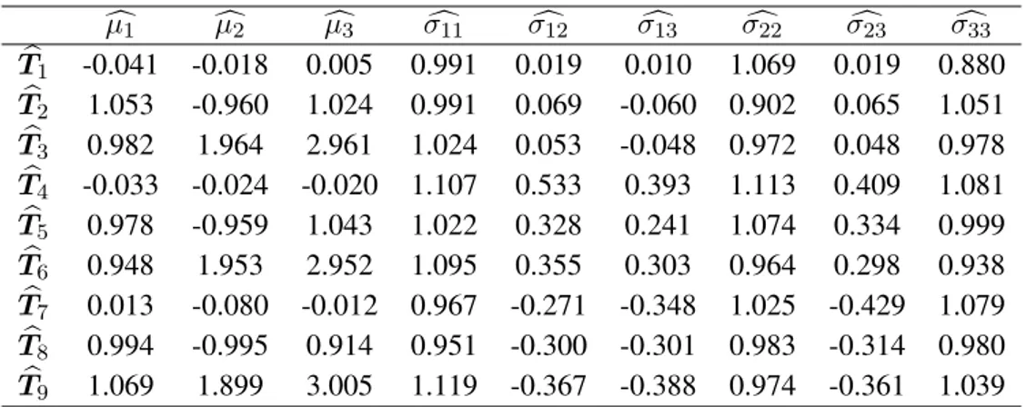
Once obtained the samples and computed the statistics we have obtained the matrix of coordinates for each population shown in Table 2.
c µ1 cµ2 cµ3 σc11 σc12 σc13 σc22 σc23 σc33 b T1 -0.041 -0.018 0.005 0.991 0.019 0.010 1.069 0.019 0.880 b T2 1.053 -0.960 1.024 0.991 0.069 -0.060 0.902 0.065 1.051 b T3 0.982 1.964 2.961 1.024 0.053 -0.048 0.972 0.048 0.978 b T4 -0.033 -0.024 -0.020 1.107 0.533 0.393 1.113 0.409 1.081 b T5 0.978 -0.959 1.043 1.022 0.328 0.241 1.074 0.334 0.999 b T6 0.948 1.953 2.952 1.095 0.355 0.303 0.964 0.298 0.938 b T7 0.013 -0.080 -0.012 0.967 -0.271 -0.348 1.025 -0.429 1.079 b T8 0.994 -0.995 0.914 0.951 -0.300 -0.301 0.983 -0.314 0.980 b T9 1.069 1.899 3.005 1.119 -0.367 -0.388 0.974 -0.361 1.039
Table 2: Final coordinates of populations.
Unbiased estimations of covariance matrices bΨi for these statistics in each
population have been obtained through 10000 bootstrap samples from each popu-lation sample. Finally using (8) we obtain the dissimilarity matrix D between the nine populations. As mentioned before and since we are working with multivariate normal distributions we can compare our dissimilarity not only with Mahalanobis distance under the assumption of a common covariance matrix, but also with Siegel distance between general multivariate normal populations as proposed by Calvo et al.(2002) and which is a lower bound of the Rao distance between multivariate nor-mal distributions that has not been obtained explicitly until now. Siegel distances have been computed following (2.6) in Calvo et al. (2002).
Table 3 shows the dissimilarities computed based on relevant features (RFD) and Siegel distances between the 9 simulated populations. In Table 4 we compare RFD dissimilarity with the usual Mahalanobis distance after estimating a pooled
covariance matrix.
Pop.1 Pop.2 Pop.3 Pop.4 Pop.5 Pop.6 Pop.7 Pop.8 Pop.9 Pop.1 0.000 1.876 3.785 0.729 1.966 3.621 1.003 2.045 5.309 Pop.2 1.672 0.000 3.509 2.158 0.468 3.581 2.101 1.039 4.674 Pop.3 2.765 2.651 0.000 3.459 3.404 0.532 5.099 4.487 1.262 Pop.4 0.644 1.888 2.622 0.000 2.158 3.189 2.260 3.105 5.447 Pop.5 1.742 0.439 2.590 1.836 0.000 3.386 2.597 1.833 4.836 Pop.6 2.682 2.679 0.494 2.477 2.569 0.000 5.145 4.787 2.291 Pop.7 0.892 1.826 3.295 1.486 2.048 3.271 0.000 1.659 6.491 Pop.8 1.715 0.824 3.063 2.130 1.215 3.121 1.510 0.000 5.535 Pop.9 3.367 3.134 0.964 3.311 3.134 1.418 3.767 3.459 0.000 Table 3: RFD dissimilarities for the 9 simulated populations in the upper part and Siegel distances in the lower part.
Pop.1 Pop.2 Pop.3 Pop.4 Pop.5 Pop.6 Pop.7 Pop.8 Pop.9 Pop.1 0.000 1.876 3.785 0.729 1.966 3.621 1.003 2.045 5.309 Pop.2 1.800 0.000 3.509 2.158 0.468 3.581 2.101 1.039 4.674 Pop.3 3.673 3.487 0.000 3.459 3.404 0.532 5.099 4.487 1.262 Pop.4 0.027 1.806 3.693 0.000 2.158 3.189 2.260 3.105 5.447 Pop.5 1.765 0.076 3.473 1.772 0.000 3.386 2.597 1.833 4.836 Pop.6 3.651 3.475 0.035 3.672 3.461 0.000 5.145 4.787 2.291 Pop.7 0.085 1.743 3.705 0.074 1.709 3.684 0.000 1.659 6.491 Pop.8 1.722 0.129 3.575 1.727 0.134 3.562 1.661 0.000 5.535 Pop.9 3.700 3.456 0.119 3.720 3.444 0.144 3.729 3.546 0.000 Table 4: RFD dissimilarities for the 9 simulated populations in the upper part and Mahalanobis distances in the lower part.
We present in Table 5 Spearman’s rank correlation coefficient between the three computed measures.
Dissimilarity (RFD) Siegel
Siegel 0.98147
Mahalanobis 0.87979 0.90862
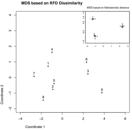
Finally in order to obtain a graphical representation of the similarities between the populations we have done a Multidimensional Scaling (MDS) based on Maha-lanobis distance and on our dissimilarity (RFD). Fig. (1) shows the result obtained for the RFD dissimilarity in the big frame and the corresponding result for Maha-lanobis distance in the upper right frame.
+ + + + + + + + + −4 −2 0 2 4 6 −2 −1 0 1 2 3 4 MDS based on RFD Dissimilarity Coordinate 1 Coordinate 2 1 2 3 4 5 6 7 8 9 + + + + + + + + + 1 2 3 4 5 6 7 8 9 −2 −1 0 1 2 3 −1.5 −0.5 0.5 1.0 1.5
MDS based on Mahalanobis distance
Figure 1: MDS based on RFD dissimilarity (big frame) and Mahalanobis distance (upper right frame) of the 9 simulated populations
5 Some applications to real data
5.1 Archaeological data
As an example, we consider the classical dataset on Egyptian skulls from five dif-ferent epochs reported by Thomson and Randall-Maciver (1905) which has been widely used in so many different works. Data consists of four measurements of 150 male Egyptian skulls from five time periods: Early Predynastic, Late Predy-nastic, 12th− 13thdynasty, Ptolemaic and Roman. The four variables measured
were: MB (Maximal Breadth of Skull), BH (Basibregmatic Height of Skull), BL (Basialveolar Length of Skull) and NH (Nasal Height of Skull).
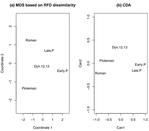
In Table 6 we show the interdissimilarity matrix obtained by the method devel-oped in the present paper with means and different coefficients of covariance ma-trices as coordinates. Figure 2a give us a representation in two dimensions through a Multidimensional Scaling of the dissimilarity matrix. Obviously the first axis can be interpreted as time, from most recent on the right to most distant on the left. The second axis has a not so clear interpretation but we observe that central values are occupied by native Egyptian populations before any foreign invasion, while late populations, where native Egyptian rulers had vanished long ago, diverge from the centerline in an almost perpendicular way. The result is quite different of that ob-tained by the standard Canonical Discriminant Analysis (CDA) as can be seen in Figure 2b.
Early P. Late P. Dyn. 12-13 Ptolemaic Roman Early P. 0.000
Late P. 2.045 0.000
Dyn. 12-13 2.546 1.785 0.000
Ptolemaic 3.595 2.934 2.244 0.000
Roman 3.636 2.155 2.261 2.642 0.000 Table 6: RFD Dissimilarities matrix for the five populations of Egyptian skulls.
5.2 Academic achievement data
The data were collected from N = 382 university students on the number of GCE A-levels taken and the students’ average grades (Mardia et al., 1979, p. 294). The students were grouped according to their final degree classification into seven
−2 −1 0 1 2 −2 −1 0 1 2 Coordinate 1 Coordinate 2 Dyn.12.13 Early.P Late.P Ptolemaic Roman
(a) MDS based on RFD dissimilarity
−1.0 −0.5 0.0 0.5 1.0 −1.0 −0.5 0.0 0.5 1.0 Can1 Can2 Dyn.12.13 Early.P Late.P Ptolemaic Roman (b) CDA
Figure 2: MDS based on RFD dissimilarity (a) and CDA (b) of the five populations of Egyptian skulls
groups: 1-I (students with degree class I), 2-II(i) (students with degree class II(i)), 3-II(ii) (students with degree class II(ii)), 4-III (students with degree class III), 5-Pass (students who obtained a ’5-Pass’), 6-3(4) (students who took four years over a three-year course) and 7-→ (students who left without completing the course). The average A-level grade obtained is a continuous variable (X1) and the number
of A-levels taken is categorized in two variables: X2 (1 if two A-levels take, 0
otherwise) and X3(1 if four A-levels taken, 0 otherwise).
We have considered as statistics the mean and standard deviation of X1 and
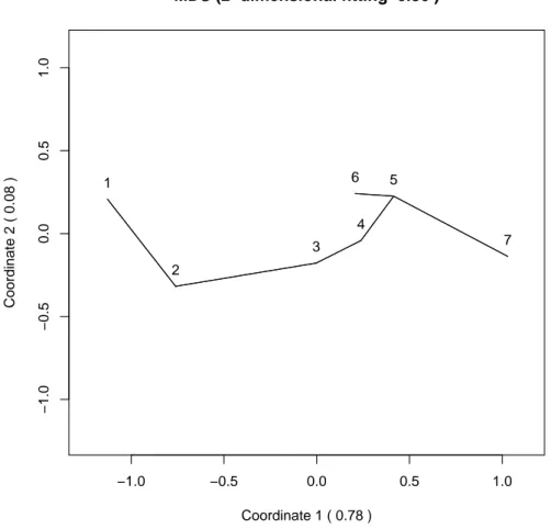
the relative frequencies for X2and X3. After obtaining the dissimilarity matrix the two-dimensional plot obtained through a classical MDS is shown in Figure 3. The minimum spanning tree of the dissimilarity matrix has been computed making use of the function mst from package ape developed in R by Paradis et al. (2009) and
the tree has been plotted on the two-dimensional scaling solution. The plot shows no distorsion in the muldimensional scaling solution, so the MDS solution reflects accurately the dissimilarity.
Mardia’s first canonical correlation solution gives the following scores to each of the degree results:
1 2 3 4 5 6 7
0 0.488 1.877 2.401 2.971 2.527 3.310 with r = 0.4 as first canonical correlation coefficient.
Mardia interpreted the scores as follows: ”The scores for I, II(i), II(ii), III and Pass come out in the natural order, but they are not equally spaced. Moreover the 3(4) group comes between III and Pass, while → scores higher than Pass. Note the large gap between II(i) and II(ii)”.
All conclusions are endorsed by our analysis as shown in Figure 3, so we think we have obtained a good representation of the seven populations based on the four chosen statistics.
−1.0 −0.5 0.0 0.5 1.0 −1.0 −0.5 0.0 0.5 1.0 Coordinate 1 ( 0.78 ) Coordinate 2 ( 0.08 ) 1 2 3 4 5 6 7 MDS (2−dimensional fitting 0.86 )
Figure 3: MDS based on RFD dissimilarity of the seven populations of university students
6 Conclusions
The proposed dissimilarity index has a reasonable behavior in all the studied cases, regardless of whether or not an adequate parametric statistical model is available for the data. The index is flexible enough to allow a wide applicability and, at the same time, maintaining a reasonable simplicity from a computational point of view.
7 References
Amari, S. (1985). Differential-Geometrical Methods in Statistics. Volume 28 of
Lecture notes in statistics, Springer Verlag, New York.
Atkinson, C. and Mitchell, A.F.S. (1981). Rao’s distance measure. Sankhy¯a, 43 A , 345–365.
Bhattacharyya, A. (1942). On a measure of divergence between two multinomial populations. Sankhy¯a, 7, 401–406.
Burbea J. (1986). Informative geometry of probability spaces. Expositiones
Mathematicae, 4, 347–378.
Burbea J. and Rao C.R. (1982). Entropy differential metric, distance and diver-gence measures in probability spaces: a unified approach. J. Multivariate
Analysis, 12, 575–596.
Calvo M., Villarroya A. and Oller J.M. (2002). A biplot method for multivariate normal populations with unequal covariance matrices. Test, 11, 143-165 Cook, D., Buja, A., Cabrera, J. and Hurley, C. (1995). Grand Tour and Projection
Pursuit. Journal of Computational Statistical and Graphical Statistics, 4 (3), 155–172.
Cubedo, M. and Oller, J.M. (2002). Hypothesis testing: a model selection ap-proach. Journal of Statistical Planning and Inference, 108, 3–21.
Friedman, J.H. (1987) Exploratory Projection Pursuit. Journal of the American
Statistical Association, 82, 249–266.
Gabriel, K.R. (1971). The biplot graphic display of matrices with application to principal component analysis. Biometrika, 58, 453–467.
Gower, J.C. and Hand, D.J. (1996). BIPLOTS. Chapman & Hall, London. Greenacre, M.J (1993). Correspondence Analysis in Practice, London: Academic
Press.
Huber, P.J. (1985). Projection Pursuit (with discussion). The Annals of Statistics, 13, 435–525.
Lindsay, B.G., Markatou, M., Ray, S., Yang, K. and Chen, S. (2008). Quadratic distances on probabilities: a unified foundationThe Annals of Statistics 36(2) 2, 983–1006.
Mahalanobis (1936). On the generalized distance in statistics. Proc. Natl. Inst.
Sci. India 2 (1) 49–55.
Mardia, K. V., Kent, J. T., and Bibby, J. M. (1979). em Multivariate Analysis, Probability and Mathematical Statistics. Academic Press, London
Mi˜narro A. and Oller J.M. (1992). Some remarks on the individual-score distance and its applications to statistical inference. Q¨uestii´o, 16, 43–57.
Oller J.M. and Corcuera J.M. (1995), Intrinsic Analysis of the Statistical Estima-tion, The Annals of Statistics 23(2), 1562–1581.
Paradis, E., Strimmer, K., Claude J., Jobb, G., Opgen-Rhein, R., Dutheil, J., Noel, Y. and Bolker, B. (2009), ape: Analyses of Phylogenetics and Evolution, URL http://CRAN.R-project.org/package=ape, R package version 2.3 Rao, C.R. (1945). Information and accuracy attainable in the estimation of
statis-tical parameters. Bull. Calcutta Math. Soc., 37, 81–91.
Thomson, A. and Randall-Maciver, R. (1905) Ancient Races of the Thebaid, Ox-ford University Press, OxOx-ford.