Output field-quadrature measurements and squeezing in ultrastrong cavity-QED

(1)

This content has been downloaded from IOPscience. Please scroll down to see the full text.

Download details:

IP Address: 134.160.214.34

This content was downloaded on 02/12/2016 at 16:33

Please note that terms and conditions apply.

Output field-quadrature measurements and squeezing in ultrastrong cavity-QED

View the table of contents for this issue, or go to the journal homepage for more 2016 New J. Phys. 18 123005

(2)

PAPER

Output

ﬁeld-quadrature measurements and squeezing in ultrastrong

cavity-QED

Roberto Stassi1,2,6

, Salvatore Savasta2,3

, Luigi Garziano2,3

, Bernardo Spagnolo1,4

and Franco Nori2,5

1 _{Dipartimento di Fisica e Chimica, Group of Interdisciplinary Theoretical Physics, Università di Palermo and CNISM, Viale delle Scienze,}

Ediﬁcio 18, I-90128 Palermo, Italy

2 _{CEMS, RIKEN, Saitama 351-0198, Japan}

3 _{Dipartimento di Fisica e di Scienze della Terra, Università di Messina, Viale F. Stagno d}_{’Alcontres 31, I-98166 Messina, Italy} 4 _{Istituto Nazionale di Fisica Nucleare, Sezione di Catania, Italy}

5 _{Physics Department, The University of Michigan, Ann Arbor, MI 48109-1040, USA} 6 _{Author to whom any correspondence should be addressed.}

E-mail:rstassi@unime.it

Keywords: quadrature measurements, squeezing, ultrastrong cavity-QED

Abstract

We study the squeezing of output quadratures of an electro-magnetic

ﬁeld escaping from a resonator

coupled to a general quantum system with arbitrary interaction strengths. The generalized theoretical

analysis of output squeezing proposed here is valid for all the interaction regimes of cavity-quantum

electrodynamics: from the weak to the strong, ultrastrong, and deep coupling regimes. For coupling

rates comparable or larger then the cavity resonance frequency, the standard input–output theory for

optical cavities fails to calculate the variance of output

ﬁeld-quadratures and predicts a non-negligible

amount of output squeezing, even if the system is in its ground state. Here we show that, for arbitrary

interaction strength and for general cavity-embedded quantum systems, no squeezing can be found in

the output-ﬁeld quadratures if the system is in its ground state. We also apply the proposed theoretical

approach to study the output squeezing produced by:

(i) an artiﬁcial two-level atom embedded in a

coherently-excited cavity; and

(ii) a cascade-type three-level system interacting with a cavity ﬁeld

mode. In the latter case the output squeezing arises from the virtual photons of the atom-cavity

dressed states. This work extends the possibility of predicting and analyzing the results of

continuous-variable optical quantum-state tomography when optical resonators interact very strongly with other

quantum systems.

1. Introduction

Recently, a new regime of cavity quantum electrodynamics(QED) has been experimentally reached in different solid state systems and spectral ranges[1–8]. In this so-called ultrastrong coupling (USC) regime, where the

light–matter coupling rate becomes an appreciable fraction of the unperturbed resonance frequency of the system, the routinely invoked rotating wave approximation(RWA) is no longer applicable and the antiresonant terms signiﬁcantly change the standard cavity-QED scenarios [9–18].

It has been shown that, in this USC regime, the correct description of the output photonﬂux, as well as of higher-order Glauber’s normal-order correlation functions, requires a proper generalization of the input– output theory for resonators[13,19,20]. Application of the standard input–output picture to the USC regime

would predict an unphysical continuous stream of output photons for a system in its ground state∣Gñ. This result stems from theﬁnite number of photons which are present in the ground state due to the counter-rotating terms in the interaction Hamiltonian[21]. Speciﬁcally, it has been shown [13,22] that the photon rate emitted

by a resonator and detectable by a photo-absorber is no longer proportional to á_{a t a t}ˆ ( ) ˆ ( )† ñ_{(as predicted by the}

standard input–output theory), where ˆa and_aˆ†_{are the photon destruction and creation operators of the cavity}

mode, but to áx t x t , whereˆ ( ) ˆ ( )- + ñ x t is the positive frequency component of the quadrature operatorˆ ( )+

OPEN ACCESS

RECEIVED

2 October 2016

ACCEPTED FOR PUBLICATION

10 November 2016

PUBLISHED

2 December 2016 Original content from this work may be used under the terms of theCreative Commons Attribution 3.0 licence.

Any further distribution of this work must maintain attribution to the author(s) and the title of the work, journal citation and DOI.

(3)

= + ˆ ( ) ˆ ( ) ˆ ( )†

x t a t a t and_{x t}ˆ ( )- =( ˆ ( ))_{x t}+ †_{, which can be different from the bare photon creation an}

destruction operators. When the coupling rate is not a negligible fraction of the bare resonance frequencies, the correct separation into positive and negative frequency operators can be performed only by including the inﬂuence of the interaction Hamiltonian. This separation can be easily performed after the diagonalization of the total system Hamiltonian.

Direct photon counting experiments provide information about the mean photon number and higher-order normal-higher-order correlations. However a complete quantum tomography of the electro-magneticﬁeld (see, e.g.,[23]) requires phase-sensitive measurements which are based on homodyne or heterodyne detection

[24,25]. These techniques enable the measurements of the mean field quadratures and their variance, e.g.,á ñxˆ andá ñ - á ñxˆ2 xˆ2_{. More generally, for an electro-magnetic}_{field-mode, it is possible to define two complementary}

ﬁeld-quadratures_Qˆ₁_and_Qˆ₂_with_{[ ˆ}_{Q Q}₁_, _{ˆ ]}₂ ₌₁_{, as}_Qˆ ₌_a_ˆ_e-f ₊_a_ˆ†_ef

1 i i andQˆ2= -i e( ˆa -if-aˆ†eif). In a

coherent state of an electro-magneticfield mode, the quantum fluctuations of the two field-quadraturesQˆ1and

ˆ

Q2are equal(DQˆ1= DQˆ2=1, where DQî= áQîñ - á ñQî

2 ₂

) and minimize the uncertainty product given by Heisenberg’s uncertainty relation DQˆ1DQˆ2=1(we use = 1). These zero-point fluctuations represent the standard quantum limit to the reduction of noise in a signal. Other minimum-uncertainty states are possible, and these occur whenfluctuations in one quadrature are squeezed at the expense of increased fluctuations in the other one[26]. Light squeezing can be realized in various nonlinear optical processes, such as parametric

down-conversion, parametric ampliﬁcation, and degenerate four-wave mixing [27–31] or in presence of

time-dependent boundary conditions[32–35]. Squeezed states of light belong to the class of nonclassical states of

light. Having a less noisy quadrature, squeezed light has applications in optical communication[36] and

measurements[36–40] and is a primary resource in continuous variable quantum information processing [38].

Squeezing of the electromagneticﬁeld has been achieved in a variety of systems operating in the optical and microwave regimes. A noise reduction of−10 dB (−13 dB is the estimation of squeezing after correction for detector inefﬁciency) has been achieved in the experiment [41]. More recently, a few experiments with

superconducting circuits[34,42] have demonstrated the possibility of obtaining much stronger squeezing in

microwaveﬁelds [43].

Here we present a theory of quadrature measurements of the outputﬁeld escaping from a resonator coupled to a generic matter system with arbitrary interaction strength, and we apply it to the analysis of squeezing. In cavity-QED systems, the squeezing effect has been usually studied by using the rotating-wave approximation [44–49]. While in the USC regime the positive frequency componentxˆ+is different from ˆa(it may contain

contributions from the creation operator of the cavityﬁeld), the quadrature operator = +_xˆ _aˆ _aˆ†=_xˆ++_{x is}ˆ -independent of the light–matter interaction strength. Hence, at a ﬁrst sight, one may expect that, in contrast to Glauber’s correlation functions, quadrature measurements can be analyzed by applying the standard input– output theory[50,51]. Here we show that this is not the case: application of the standard input–output picture to

the analysis of quadrature measurements in the USC regime leads to incorrect results. We also observe that the calculation of quadrature expectation values by means of the generalized input–output relations (working for arbitrary light–matter coupling) presents some additional complications compared to that of normal-order correlations. In particular, the resulting quadrature expectation values contain products of system and input operators and thus cannot be directly derived within the master equation approach. The present analysis is of particular interest for the description of measurements in circuit-QED systems, where output quadrature measurements are generally employed since efficient microwave photon-counting detectors are not currently available. However, well-developed linear amplifiers allow for the efficient measurement of the field-quadrature amplitudes[25,42,52,53]. Using input–output theory [51], one can show that the full information about the

intracavityﬁeld-mode is contained in the moments and cross-correlations of the time-dependent output quadrature amplitudes. It has been demonstrated experimentally that correlation-function measurements based on quadrature amplitude detection are a powerful tool to characterize quantum properties of propagating microwave-frequency radiationﬁelds [52]. Hence a general method to calculate these time-dependent

moments, when the resonator interacts with one or more artiﬁcial atoms in the USC regime, is highly desirable for the analysis of the output microwaveﬁeld in circuit-QED systems.

We apply the theoretical framework developed here to analyze three different cases:(i) we analyze the output ﬁeld-quadratures for a system in its ground state. It is know that the ground state of a system in the USC regime is a squeezed vacuum state[19], where the amount of squeezing depends on the coupling strength and on the

detuning between the cavity mode and the matter-system resonances. A correlation-function analysis of the quadratures of microwavefields has been exploited for measurements of vacuum fluctuations and weak thermal fields [54]. Hence the question arises if it is possible to detect such vacuum squeezing. Here, under quite general

hypotheses, we demonstrate that for arbitrary cavity-embedded quantum systems, independently on the coupling rate, no squeezing can be found in the outputﬁeld quadratures if the system is in its ground state. (ii) We study a coherently excited cavity interacting with an artiﬁcial two-level atom. Recently, it has been shown

(4)

that superconducting artiﬁcial atoms, subject to parity-symmetry-breaking and ultrastrong coupled to superconducting resonators, can display two-photon vacuum Rabi oscillations[22]. However, two-photon

correlations cannot directly be detected in these systems. We show that quadrature-noise measurements can provide an alternative direct probe. This process can give rise to a high degree of squeezing in presence of a single two-level system, just exciting the qubit with a classical microwave pulse.(iii) As a further example of the developed framework, we analyze the output squeezing from a resonator interacting with a cascade-type three-level system.

We start out, in section2, with the squeezing of the ground state of the Rabi Hamiltonian. In section3we present a theoretical framework of the outputﬁeld quadratures. In section4this theoretical approach is applied to single-atom USC cavity-QED systems. Finally, in section5we present our conclusions.

2. Squeezing of the ground state of the Rabi Hamiltonian

The Hamiltonian of the quantum Rabi model( = 1) [55,56] is given by

w w s s = + + W + ˆ _{ˆ ˆ}† _ˆ _{( ˆ}† _{ˆ) ˆ} _{( )} H a a a a 2 z x, 1 R c q R

where ˆa and_aˆ†_{are, respectively, the annihilation and creation operators for the cavity}_{ﬁeld of frequency}_w c. The

Pauli matrices are deﬁned as s = ñá - ñáˆz ∣e e∣ ∣g g∣and sˆx=sˆ++sˆ-= ñá + ñá∣e g∣ ∣g e∣, in terms of the atomic ground(∣gñ) and excited (∣eñ) states. The parameter wqdescribes the transition energy of the two-level system

and WRis the coupling energy between the atomic transition and the cavityﬁeld.

Owing to the presence of the so-called counter-rotating terms, saˆ ˆ-andaˆ ˆ†s+, in the Rabi Hamiltonian, the

operator describing the total number of excitations,_Nˆ =_{a a}ˆ ˆ† + ñá∣_{e e , does not commute with}∣ _H_ˆ

Rand as a

consequence the eigenstates ofHˆRdo not have a deﬁnite number of excitations [21], however the system

described by the Hamiltonian in equation(1) conserves the parity of the number of excitations. For instance the

resulting ground state, in terms of the bare cavity and qubit states, is a superposition of an even number of excitations[21],

å

ñ º ñ = ñ + + ñ = ¥ ∣G ∣˜0 (c˜ ∣g, 2k c˜ ∣e, 2k 1 ,) ( )2 k g k e k 0 ,2 0 , 0

where the second entry in the kets provides the photon number. The coefﬁcients of this expansion can be calculated diagonalizing numerically the Rabi Hamiltonian in equation(1) (see, e.g., [21,22]). When the

coupling rate WRis much smaller than the bare resonance frequencies of the two subsystemswcand wq, only ˜

c_g,00

is signiﬁcantly different from zero and the ground state reduces to ñ∣˜0 ∣g, 0 , which is that of the Jaynesñ – Cummings model, derived from the Rabi Hamiltonian after dropping the counter-rotating terms. When the coupling rate WRapproaches and exceed 10% of the bare frequencies of the subsystems, that is USC regime,

contributions withk¹0 in equation(2) become not negligible. One consequence is that the mean photon

number in the ground state á₀˜∣ ˆ ˆ∣˜_{a a}† _{0 becomes different from zero. Moreover, the ground state displays a certain}ñ

amount of photon squeezing. Considering the intracavity-ﬁeld quadrature_qˆ =_i( ˆ_a†-_aˆ)

2 , its variance

= á˜∣ ˆ ∣˜ñ - á˜∣ ˆ ∣˜ñ

s2 0q₂20 0q202(notice that á0˜∣ ˆ ∣˜q20ñ =0) turns out to be below the standard quantum limit value 1.

Figure1displays the numerically calculated ( )=

-s2n s2 1as a function of the normalized couplingWR wc

and detuningD wc=(wq -w wc) c. For small values of the normalized coupling, the variance approaches the

standard quantum limit.

We notice that, increasingWR wc, the variance decreases below the standard quantum limit, reaching a

lowest value of about−0.35, atWR wc 1.05and at a positive detuningD wc 0.76. Further increasing the

coupling, especially at zero and negative detuning, results into an increase of the variance s2, caused by quite large

contributions in∣˜0ñof terms with an odd number of photons.

This noise increase can be understood noticing that the noise reduction originates from the terms yá ∣ ˆ ∣a2yñ_,

and the operatoraˆ2_{connects only terms in the quantum states}_∣_yñ_{differing by two photons. Hence squeezing}

can be larger for states with either an even or an odd number of photons. In the next section we will show that such a ground-state squeezing actually does not give rise to an observable output squeezing.

3. Output

ﬁeld quadratures

According to the input–output theory for general localized quantum systems interacting with a propagating quantumfield, the output field operator can be related through a boundary condition to a system operator and the inputfield operators [57]. In order to be specific, we consider the case of a system coupled to a semi-infinite

transmission line[57], although the results obtained can be applied or extended to a large class of systems. While

(5)

quantumﬁeld (e.g., the transmission line) is weak. To derive the input–output relations we couple the system to a quantumﬁeld made of an assembly of harmonic oscillators. The total Hamiltonian of the system can be written as

= + +

ˆ ˆ ˆ ˆ _{( )}

H HS HF H ,SF 3

whereHˆSand ˆHFare the system andﬁeld Hamiltonian and where the interaction between the system and the

ﬁeld can be expressed in the rotating wave approximation as 

ò

w w w w w = ¥ - - + ˆ _{( )} _{[ ˆ ˆ ( )} _{ˆ ˆ ( )]}† _{( )} H i d k v X b X b 2 , 4 SF 0

where v is the speed of the travelingﬁeld, e.g., the speed of light in the transmission line.

In the above equation,bˆ ( )w andk( )w are the annihilation operator and the spectral density for the harmonic oscillators that describe the outputfield,X andˆ+ Xˆ-are the positive and negative frequency components of the generic system operatorXˆcoupled to thefield. These components can be obtained expressingXîn the eigenvectors basis ofHˆSas

å

= ñá + < ˆ _∣ _∣ _{( )} X X i j , 5 i j ij

and_Xˆ-=( ˆ )_X+†_{. Here the eigenstates of}_H_ˆ

Sare labeled according to their eigenvalues such thatwk>wjfor >

k j. We observe that the rotating wave approximation used in equation(A4) is based on the separation into

positive and negative frequency operators of the system operatorXˆafter the system diagonalization. The standard RWA is instead based on the separation into bare positive(destruction) and negative (creation) components of theﬁeld operator coupled to the external modes, without including its interaction with other components of the system.

The positive frequency component of the input and outputﬁelds can be written as 

ò

w pw w w = ¢ - - ¢ + ¥ ˆ ₍ ₎_{( )} _{ˆ (} ₎ _[ ₍ _] _{( )} A t 1 b t t t 2 d , exp i , 6 in out 0

while the negative frequency componentAˆin out-( ) =( ˆAin out+( ))†, so that = +

+

-ˆ ₍ ₎_{( )} ˆ _{( )} ˆ _{( )}

( ) ( )

Ain out t Ain out t Ain out t , in

which ¢ <t t(the input) is a ﬁxed initial time and ¢ >t t(the output) is assumed to be in the remote future [57].

Formally solving the Heisenberg equations of motion forbˆ ( )w , the input–output relations for the positive and

negative components of theﬁelds can be obtained [22]

g

=

-  

ˆ _{( )} ˆ _{( )} _{ˆ ( )} _{( )}

A_out t A_in t X t , 7

where for the sake of simplicity theﬁrst Markov approximation, wk( )= 2g p, has been adopted. However, the present analysis can be easily extended beyond this approximation. Equation(7) shows that the positive

frequency output operator can be expressed in terms of the positive frequency input operator and the positive frequency system operator coupled to the propagatingﬁeld. If the system consists of an empty single-mode resonator, thenXˆ+µa, being ˆˆ a the destruction operator of the cavity mode. If instead the cavity mode is

Figure 1. Normally-ordered variance_s( )n =_s -₁

2 2 of the cavity-ﬁeld quadraturexˆ2=i( ˆa†-aˆ), calculated in the ground state∣˜0ñof the Rabi Hamiltonian, as a function of the normalized coupling rateWR wcand cavity-atom detuningDwc=(wq-w wc) c.

(6)

coupled to another quantum system, e.g., an atom,X will be different from ˆa, and may also containˆ+

contributions from_aˆ†_{. In this case, the positive component of the output}_{ﬁeld may contain contributions from}

the creation operator of the cavityﬁeld, in contrast to ordinary quantum optical input–output relation-ships[27,51].

We deﬁne the output quadrature operators ˆ ( )Q t1 and ˆ ( )Q t2 as

= + = - -+ _{- G} - _G + _{- G} - _G ˆ ( ) ˆ _{( )} ˆ _{( )} ˆ ( ) [ ˆ ( ) ˆ ( ) ] ( ) ( ) ( ) ( ) ( ) Q t A t A t Q t A t A t e e i e e 8 t t t t 1 out i out i 2 out i out i so that =  G  ˆ _{( )} _{[ ˆ ( )} _{ˆ ( )]} _[ _{( )]} _{( )} A t 1 Q t Q t t 2 i exp i , 9 out 1 2

whereG( )t = W +t j. HereΩ and j are, respectively, the frequency and the phase of the local oscillator ﬁeld employed for the squeezing measurements[29]. It is possible to change from one quadrature to the other by

applying a p 2 rotation to one of the two quadratures, e.g., by changing the reference phasej.

Let us now consider theﬁeld-quadrature varianceS ti( ,t)= áQ tˆ ( ) ˆ (i ,Q ti +t)ñ. Using equation(9), it can be expressed in terms of the output operators,

t t t t t = á + ñ + á + ñ + á + ñ + á + ñ + + _{- G} - - _G + - - + ( ) ˆ ( ) ˆ ( ) ˆ ( ) ˆ ( ) ˆ _{( ) ˆ} ₍ ₎ ˆ _{( ) ˆ} ₍ ₎ ₍ ₎ S t A t A t A t A t A t A t A t A t , e e . 10

i out out 2i out out 2i

out out out out

By using the input–output relation (7), each term in the above equation can be written in terms of input and

system operators. For example, theﬁrst expectation value in the r.h.s. of equation (10) becomes,

t t g t g t g t á + ñ = á + ñ + á + ñ - á + ñ - á + ñ + + + + + + + + + + ˆ _{( ) ˆ} ₍ ₎ _{ˆ ( ) ˆ (} ₎ _{ˆ ( ) ˆ (} ₎ ˆ ( ) ˆ ( ) ˆ ( ) ˆ ( ) ( ) A t A t A t A t X t X t A t X t X t A t . 11 out out in in in in

We observe that equation(11) contains expectation values involving products of input and system operators.

Even considering the important case of a vacuum input port, the mixed termáAˆ ( ) ˆ (in+t X+t+t)ñis in general different from zero and cannot be directly calculated by the master equation approach, which does not calculate mixed bath-system correlations. This problem can be solved by deriving the commutation relations between system and input operators. By using equation(6) and the expression of the ﬁeld operator wbˆ ( ), obtained from solving the Heisenberg equation, we arrive at the following commutation relation between any system variable

ˆ ( )

Y t and the inputﬁeldsAˆ ( )_int

g

=

- 

[ ˆ ( ) ˆY t ,A_in( )]s u t( s Y t)[ ˆ ( ) ˆ ( )],X s , (12) whereu t( -s)is equal to 1 if >t s,1

2if t=s, and 0 if <t s. This commutation relation, which holds for

arbitrary light–matter couplings, can be considered to be the generalization of an analogous commutation relation obtained within the standard input–output framework [50]. Its derivation is described in appendixA.

Making use of the input–output relations (7) and of the commutation relations (12), we can proceed to

calculate the outputﬁeld quadrature variancesS ti(,t)= áQ tˆ ( ) ˆ (i ,Q ti +t)ñin terms of correlation functions involving only input operators or system operators. Here we used áA Bˆ, ˆñ = áABˆ ˆñ - á ñá ñA Bˆ ˆ. Considering an input in a vacuum or a coherent state, theﬁeld-quadrature variances can be expressed as

  t g t t t t t = á + ñ + á + ñ + á + ñ + á + ñ + á + ñ + + _{- G} - - _G - + - + + -( ) [ ˆ ( ) ˆ ( ) ˆ ( ) ˆ ( ) ˆ ( ) ˆ ( ) ˆ ( ) ˆ ( ) ] ˆ ( ) ˆ ( ) ( ) ( ) ( ) S t X t X t X t X t X t X t X t X t A t A t , , e , e , , , , 13 t t 1 2i 2i in in

where  is the time-ordering operator that rearranges the creation operators in the forward time, and also the annihilation operators in the backward temporal order. To obtain S2we can apply a p 2 rotation to

equation(13). For equal-time correlation functions (t = 0), we have g = á ñ + á ñ + á ñ + á ñ + + - G - - G - + + -( ) [ ˆ ( ) ˆ ( ) ˆ ( ) ˆ ( ) ˆ ( ) ˆ ( ) ] ˆ ( ) ˆ ( ) ( ) ( ) ( ) S t X t X t X t X t X t X t A t A t , e , e 2 , , . 14 t t 1 2i 2i in in

The last term in equation(14) áAˆin+,Aˆin-ñdescribes the quantum noise of the input in the vacuum state. We

observe that, according to equation(5), the operatorX can induce only downward transitions from higherˆ+

energy to lower energy levels. Hence, when it is applied to the ground state, it automatically gives zero: ñ =

+

ˆ ∣ ( )

(7)

If the system starts in its ground state, in the presence of a vacuum input, it will remain there. Using then equation(15), the term áX tˆ ( ) ˆ ( )- ,X+t ñin equation(14) becomes zero and the output noise in equation (14)

coincides with the input one:S t1( )= áAˆ ( ) ˆ ( )in+t Ain-t ñ. From equations(14) and (15) we can thus formulate the

following general statement: Any open system in its ground state, i.e.,Xˆ+∣0ñ =0, does not display any output squeezing, even if its ground state is a squeezed state. Equation(14) holds for general open quantum systems,

independently on their composition in subsystems and the degree of interaction among the different subsystems. This absence of output ground-state squeezing has been previously shown in different interacting harmonic systems[19,58,59].

In order to compare this result with previous descriptions for optical resonators, we consider the case where ˆ

Xdescribes theﬁeld of a single-mode cavity:_Xˆ =_{X x}ˆ=_{X a}( ˆ +_aˆ )†

0 0 . Here X0denotes the zero-point

ﬂuctuation amplitude of the resonator. Equation (14) can be expressed as g = á ñ + á ñ + á ñ + á ñ + + - G - - G - + + -( ) [ ˆ ( ) ˆ ( ) ˆ ( ) ˆ ( ) ˆ ( ) ˆ ( ) ] ˆ ( ) ˆ ( ) ( ) ( ) ( ) S t X x t x t x t x t x t x t A t A t , e , e 2 , , . 16 t t 1 02 2i 2i in in

If the interaction of the resonator with other quantum systems is not in the USC regime,xˆ+=aˆand_xˆ-=_{a .}ˆ†

The noise reduction with respect to the vacuum input can be expressed in terms of the following normally-ordered variance g = - á ñ + -( ) ( ) ˆ ( ) ˆ ( ) ( ) ( ) S t S t A t A t X , . 17 in i in in 02

For a resonator not in the USC regime, an ideally squeezed quadrature corresponds to ( )=

-S_in 1, while for a resonator in the ground stateS_i( )n =0.

4. Squeezing of output

ﬁeld-quadratures in the USC regime

Here we apply the theoretical framework developed in section3to study the outputfield-quadrature variances in single-atom USC cavity-QED systems. Wefirst consider the case of a flux qubit artificial atom coupled to a

l 2 superconducting transmission-line resonator, when the frequency of the resonator is near one-half of the

atomic transition frequency(see ﬁgure2). Recently it has been shown [60] that this regime can strongly modify

the concept of vacuum Rabi oscillations, enabling two-photon exchanges between the qubit and the resonator. Here we show that such conﬁguration can provide a very large amount of squeezing, although the system has only one artiﬁcial atom and displays a moderate coupling rateWR wc~ 0.1. Then, we will study the output squeezing of a cascade three-level system where only the upper transition is coupled to the optical resonator.

In order to describe a realistic system, the dissipation channels need to be taken into account. For this reason all the dynamical evolutions displayed below have been numerically calculated solving the master equation



rˆ˙ ( )t =i[ ˆ ( )r t ,H]+ å_i irˆ ( )t [22,61,62], whereiis a Liouvillian superoperator describing the cavity and

atomic system losses(see appendixA). All calculations have been carried out by considering zero temperature

reservoirs.

4.1. Two-photon Rabi oscillations

We now consider aﬂux qubit ultrastrongly coupled to a coplanar resonator [2]. This quantum circuit is

analogous to a cavity-QED system, where theflux qubit with its discrete anharmonic energy levels represents the artificial atom and the coplanar resonator the optical cavity (see figure2). Recently it has been shown that this

system paves the way to anomalous vacuum Rabi oscillations, where two or more photons are jointly and reversibly emitted and reabsorbed by the qubit[60,63].

This quantum circuit can be described by the following extended Rabi Hamiltonian[2]

w w s s q s q s

¢ = + + -+ W + +

ˆ _{ˆ ˆ}† _{ˆ ˆ} _{( ˆ}† _ˆ)( _ˆ _{ˆ )} ₍ ₎

HR ca a q R a a cos x sin z . 18

In this system both the number of excitations and parity symmetry are no longer conserved and transitions which are forbidden in natural atoms become available[64]. The angle θ as well as the qubit resonance frequency

depend on theﬂux offset dF º F - Fq ext 0, where Fextis the external magneticﬂux threading the qubit and F0is

theﬂux quantum. A ﬂux offset dF = 0q implies q = 0. In this caseHR¢reduces to the standard Rabi

Hamiltonian(1). We choose the labeling of the eigenstates ñ∣˜i and eigenvalues w˜jofHR¢such that wk˜>wj˜ fork˜>j .˜

The lowest eigenenergy offsets with respect to the ground energy w_j˜-w₀˜as a function of the qubit

transition frequency wqare shown inﬁgure2. Looking at the numerically calculated eigenvectors, theﬁrst

excited state,∣ ˜1ñ, contains a dominant contribution from the bare state∣g, 1ñ,( ñ∣ ˜1 ∣g, 1ñ). The ﬁgure also shows an avoided crossing whenwq» 2wc. The splitting can be attributed to the resonant coupling of the states

(8)

ñ

∣e, 0 and∣g, 2ñ, although the USC regime implies that the resulting dressed states∣˜2ñand∣˜3ñcontain also small contributions from other bare states, as∣g, 1ñand∣e, 1ñ. This splitting cannot be found in the rotating wave approximation, where the coherent coupling between states with a different number of excitations is not allowed, nor does it occur with the standard Rabi Hamiltonian(q = 0).

We consider a system initially in the ground state. Excitation occurs by direct optical driving of the qubit via a microwave antenna. The corresponding driving Hamiltonian is

 w s

=

ˆ _{( )} ₍ _{) ˆ} ₍ ₎

Hd t cos t x, 19

where ( )t =Aexp[ (- -t t0)2 (2t2)] (t 2p)describes a Gaussian pulse. Here A andτ are the amplitude and the standard deviation of the Gaussian pulse, respectively. We consider the zero-detuning case,

corresponding to the minimum energy splitting W2 effbetween the two split levels(∣˜2ñand∣˜3ñ) in ﬁgure2(b). The

central frequency of the pulse has been chosen to be in the middle of the two split transition energies:

w =(w₃˜+w₂˜) 2-w₀˜. Ifτ is much smaller than the effective Rabi period, t T_R =2p W_eff, the driving

pulse is able to generate an initial superposition with equal weights of the states∣˜2ñand∣˜3ñ, which will evolve displaying two-photon quantum vacuum oscillations[60]. Figure3(a) displays the resulting qubit population

(red dashed curve) and mean photon number (blue continuous) after a pulsed excitation with an effective pulse area =p 3. Figure3(b) shows the normally-ordered variance of the two orthogonal output ﬁeld quadratures

( )

S1n (blue continuous curve) andS2( )n (dotted red). Both the two quadratures display a signiﬁcant amount of

squeezing when the mean photon number is maximum. It is interesting to see that the periodicity of the two variances is twice the Rabi period TR. This can be understood noticing that after the excitation, the quantum state

is a superposition of the ground state∣˜0ñand the excited states∣˜2ñand∣˜3ñ. After one Rabi oscillation, the excited states acquire aπ phase shift. A second Rabi oscillation is needed to recover the initial phase. The dynamics of the corresponding variances(not shown here) calculated by using ˆa and_aˆ†_{, instead of}_x_ˆ+_and_x_ˆ-_{, are affected by fast}

oscillations.

Figure 2._{(a) Sketch of a cavity-embedded two-level system. (b) Frequency differences with respect to the ground state:}

wk˜ ˜0=wk˜-w0˜for the lowest-energy dressed states ofHˆR¢as a function of the qubit transition frequency w wq c. We consider a normalized coupling rateWR wc= 0.15between the qubit and the resonator. In correspondence of the avoided level crossing(at

(9)

This periodic and alternating squeezing of the two quadratures can be better understood by a simpliﬁed effective model assuming that

ñ ñ + ñ ñ ñ - ñ   ∣˜ (∣ ∣ ) ∣˜ (∣ ∣ ) ( ) e g e g 2 1 2 , 0 , 2 , 3 1 2 , 0 , 2 . 20

Considering the qubit initially prepared in the superposition state y∣ (t=0)ñ =a∣g, 0ñ +b∣e, 0ñ(with

a + b =

∣ ∣2 ∣ ∣2 1_{), the resulting time evolution of the system state is, to a good approximation,}

y ñ =a ñ +b W ñ + W ñ

∣ ( )t ∣g, 0 [cos( efft e)∣ , 0 sin( efft g)∣ , 2 ,] (21) where W2 effis the minimum energy splitting inﬁgure2(b). Att=p (2Weff), the resulting state is

a b

ñ ñ + ñ

∣g ( ∣0 ∣2 ), which is a squeezed photon state, reaching a maximum squeezing for a  1 3. 4.2. Cascade three-level system

We consider a three-level(∣sñ,∣gñand ñ∣ )e atom-like system with the upper transition(∣gñ « ñ∣ )e ultrastrongly coupled with a mode of the resonator and a lower transition which does not interact with the resonator, as schematically shown inﬁgure4. The peculiar optical properties of this system have been analyzed calculating the dynamics of the populations and of normal-order correlation functions[15,65,66]. The system Hamiltonian is

å

w w s s s = + + W + + a a aa = ˆ _{ˆ ˆ}† _ˆ _{( ˆ} _{ˆ )( ˆ}† _{ˆ )} ₍ ₎ H a a a a , 22 s g e eg ge c , , R

where wa(a = s g e, , ) are the bare frequencies of the atom-like relevant states, and sab=∣a bñá ∣describes the transition operators(projection operators if a=b) involving the levels of the quantum emitter. The

Hamiltonian can be separated asHˆ =HˆR+Hˆs, whereHˆRis the well known Rabi Hamiltonian, equation(1),

andHˆs =w ss ssˆ . As a consequence, the total Hamiltonian is block-diagonal and its eigenstates can be separated

Figure 3.(a) Temporal evolution of the cavity mean photon number áX Xˆ ˆ- +ñ_{(blue continuos curve) after the arrival of a Gaussian}

pulse exciting the qubit. The pulse has an affective areap 3and central frequency(w3˜+w2˜) 2.(b) Time evolution of the

normally-ordered variancesS( )n( )t

1 (blue continuos curve) andS2( )n( )t (red dashed curve). Here, the resonator and qubit damping rates are

g =g =_1.8´₁₀-w

c q 4 c. The yellow background,(shaded region) shows the region with negative ordinates corresponding to squeezed states.

(10)

into a non-interacting sector∣s n, ñ, with energyws + nwc, where n labels the cavity photon number, and into

dressed atom-cavity states ñ∣˜j , resulting from the diagonalization of the Rabi Hamiltonian. We consider the

system initially prepared in the∣˜0ñstate. Preparation can be accomplished by simply exciting the system initially in the ground state∣s, 0 with añ π pulse of central frequencyw₀˜ -w_s. Then the qubit is excited by two additional

pulses with central frequencies w₁=w₀˜ -2w_cand w₂=w˜₀-w_s. The driving Hamiltonian is

 w  w s s

= + +

ˆ _{[ ( )} ₍ ₎ _{( )} ₍ _{)]( ˆ} _{ˆ )} ₍ ₎

Hd 1t cos 1t 2 t cos 2t gs sg , 23

where 1,2( )t =A1,2exp[ (- -t t0)2 (2t2)] (t 2p)describes Gaussian pulses. While the transition

ñ  ñ

∣˜0 ∣s, 0 is allowed in the weak-coupling regime or even in the absence of a resonator, the matrix element for the transition ñ ∣˜0 ∣s, 2 vanishes for a zero coupling rate and is negligible until Wñ Rreaches at least 10% ofwc.

Speciﬁcally: s s s s á + ñ = á + ñ = ∣( ˆ ˆ )∣˜ ∣( ˆ ˆ )∣˜ ( ) ˜ ˜ s c s c , 0 0 , , 2 0 . 24 gs sg g gs sg g ,0 0 ,2 0

In order to obtain a quantum superpositioncosf ∣s, 0ñ + sinf ∣s, 2 via the dressed vacuum state ññ ∣˜0 , the pulse amplitudes have to satisfy the following relationship:A c1 _g0˜,0 A c2 _g˜0,2=tanf. In order to obtain large squeezing, we choose the driving amplitude such thattanf » 2 2, corresponding to the angle where squeezing for this superposition state is maximal.

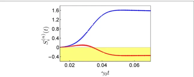
Figure5shows the time evolution of the normally-ordered variancesS₁( )n (blue upper curve) andS₂( )n (red

lower curve) calculated using the correct positive and negative operatorsX+andX-, with reference frequency

w

W = c. The squeezing displayed inﬁgure5starts with the exact value for t=0,S1( )n = S2( )n = 0, and it

does not present anyfictitious fast oscillation. On the contrary, with the use of the standard operators, see appendixC, the squeezing starts with afictitious value less than zero and shows large fictitious oscillations.

Figure 4.(a) Sketch of a cavity-embedded three-level system. Only the upper transition ñ « ñ∣g ∣e interacts with the cavity mode. The

lowest energy state of the three-level system is ñ∣s .(b) Energy spectrum ofHˆas a function of the coupling strengthWR wc, with

wgs= 3.5wcandweg=wc. The red horizontal lines represent the non-interacting states∣s n, ñ, the blue curve is the lowest-energy atom-cavity dressed state∣˜0ñ. The black arrows indicate the transitions stimulated by the driving pulses.

(11)

5. Conclusions

We have derived a generalized theory of the outputfield-quadrature measurements and squeezing in cavity-QED systems, valid for arbitrary cavity-atom coupling rates. In the USC regime, where the counter-rotating terms cannot be ignored, the standard theory predicts a large amount of squeezing in the outputfield, even when the system is in its ground state. Here we have shown that, in this case, no squeezing can be detected in the output field-quadratures, independently of the system details. We have applied our theoretical approach to study the output squeezing produced by an artificial two-level atom embedded in a coherently excited cavity. We showed that, a large degree of squeezing can be obtained with this elementary quantum system. We also studied the outputfield-quadratures from a cavity interacting in the USC regime with the upper transition of a cascade-type three-level system. The numerical results have been compared with the standard calculations of output

squeezing(see ﬁgure5). The approach proposed here can be directly applied also to resonators displaying

ultrastrong optical nonlinearities[67]. This work extends the possibilty of predicting and analyzing output-ﬁeld

correlations when optical resonators interact very strongly with other quantum systems.

Acknowledgments

We thank Professor Adam Miranowicz for very useful discussions. This work is partially supported by the RIKEN iTHES Project, the MURI Center for Dynamic Magneto-Optics via the AFOSR award number FA9550-14-1-0040, the IMPACT program of JST, a Grant-in-Aid for Scientiﬁc Research (A), CREST, the John

Templeton Foundation, and from the MPNS COST Action MP1403 Nanoscale Quantum Optics.

Appendix A. Commutation relations

Here we derive the commutation relation(12) among the positive component of the input ﬁeldAˆ ( )in+ t and any

system operator ˆ ( )Y t . The calculation for the negative component can then be obtained simply by Hermitian

conjugation. The total Hamiltonian that describes the coupling between the system and a bath of harmonic oscillators is

= + +

ˆ ˆ ˆ ˆ ₍ ₎

H HS HF H ,SF A1

whereHˆSis an arbitrary system Hamiltonian, ˆHFis the Hamiltonian that describes the bath:



å

w = ⎜⎛ + ⎟ ⎝ ⎞⎠ ˆ ˆ ˆ† ₍ ₎ H b b 1 2 , A2 n n n n F

Figure 5. Time evolution of the normally-ordered variances_S( )n

1 (blue upper curve) andS2( )n (red lower curve) calculated using the correct positive and negative operators for reference frequencyW =wc. The system is initially prepared in the lowest-energy dressed state∣˜0ñ. The qubit is excited by two pulses with central frequencies w1=w0˜-2wcand w2=w0˜-ws, at the time

g_t =_2.6´₁₀

-0 1 2and g0 2t =3.8´10-2, respectively, and with amplitude such thattanf » 2 2. The damping rates are

g =g =g = ´₂ ₁₀-w

eg gs

(12)

and the interaction HamiltonianHˆSFis 

å

w = -ˆ _{( ˆ} _{ˆ ) ˆ} ₍ ₎ H i k b b X 2 , A3 n n n n n SF

whereXˆis the system variable that interacts with the bath. In the basis that diagonalizes the system Hamiltonian ˆ HS, we have = + + -ˆ ˆ ˆ X X X , withXˆ+= åi j< X iij∣ñáj∣and = - + ˆ _{( ˆ )}†

X X . In the continuum limit for n and in the RWA, the interaction Hamiltonian in equation(A3), can be expressed as



ò

w w w w w = ¥ - - + ˆ _{( )} _{[ ˆ ˆ ( )} _{ˆ ˆ ( )]}† ₍ ₎ H i d k X b X b 2 . A4 SF 0

We observe that the RWA has been applied only after expressing the system operators in equation(A3) in the

dressed basis, so that the resulting operatorsX have a deˆ ﬁnite positive/negative frequency. Observing that the

inputﬁeldAˆ ( )_in+t is a continuous superposition of the initial-time destruction operatorsbˆ (w,t0)(see equation(6)), we can obtain an expression for it by solving the following Heisenberg equation of motion:

 w = w ˆ˙ ( ) [ ˆ ˆ ( )] ( ) b i H b, . A5 We obtain: 

ò

w = w w - + w w ¢ -w - ¢ + ¢ ˆ ( ) ˆ ( ) ( ) ( ) ( )ˆ ( ) ( ) b ,t b ,t e k t X t 2 d e . A6 t t t t t t 0 i 0 i 0 0

Now we can calculate[ ˆ ( ) ˆ ( )]Y t ,Ain+ t . From the deﬁnition of the positive-frequency component of the input

ﬁeldAˆ ( )_in+t , we obtain: 

ò

w pw w  = w + ¥ _- -[ ˆ ( ) ˆ_{Y t} _A ( )]_t ( )[ ˆ ( ) ˆ ( )] ( ) v Y t b t , 1 2 d e , , . A7 t t in 0 i 0 0

Replacingbˆ (w,t0)from equation(A6):

ò

p w w  = ¢ w ¢ + ¥ - - ¢ + [ ˆ ( ) ˆY t A ( )]t ( ) ( )[ ˆ ( ) ˆ ( )] ( ) v k t Y t X t , 1 2 2 d t d e , . A8 t t t in 0 i 0

Applying theﬁrst Markov approximation wk( )= 2g p, the above expression becomes

ò

p g _w  = ¢ ¢ w + + ¥ - - ¢ [ ˆ ( ) ˆY t A ( )]t [ ˆ ( ) ˆ ( )] ( ) ( ) v t Y t X t , 1 2 t d , d e . A9 t t t in 0 i 0

We notice that the positive-frequency operatorX t on the r.h.s. of equation+( )¢ (A9) is a superposition of

oscillating phasese- ¢ ¢iwt (beingw¢a generic positive frequency). Hence the time integral on the r.h.s. of equation(A9) contains terms oscillating asei(w w- ¢ ¢)t. Those slowly-oscillating terms with w» ¢ provide thew larger contributions to the integral. If we extend the frequency integral to the-¥limit, we are adding rapidly-oscillating termse-i(w+ ¢ ¢w)t, which provide negligible contributions. After the integral is extended to the-¥ limit, we observe that theω-integral is now equal to pd - ¢2 (t t), and weﬁnally obtain:

g = -+ + [ ˆ ( ) ˆY t A ( )]s ( )[ ˆ ( ) ˆ ( )] ( ) v u t s Y t X t , in , , A10 whereu t( -s)is equal to 1 if >t s,1 2if t=s, and 0 if <t s.

Appendix B. Master equation

In the USC regime, owing to the high ratioWR wc, the standard approach fails to correctly describe the

dissipation processes and leads to unphysical results as well. In particular, it predicts that even at T=0, relaxation would drive the system out of its ground state∣Gñgenerating photons in excess to those already present.

The right procedure that solves such issues consists in taking into account the atom-cavity coupling when deriving the master equation after expressing the Hamiltonian of the system in a basis formed by the eigenstates

ñ

∣j of the Rabi HamiltonianHˆR. The dissipation baths are still treated in the Born-Markov approximation.

Following this procedure it is possible to obtain the master equation in the dressed picture[62]. For a T=0

reservoir, one obtains:

 

(13)

Here aandxare the Liouvillian superoperators correctly describing the losses of the system where

srˆ ( )t = åj k j, _> Gsjk[∣j kñá ∣] ˆ ( )r t fors=a,s-and [ ˆ ] ˆr= ( ˆ ˆ ˆr -rˆ ˆ ˆ - ˆ ˆ ˆ)r

† † †

O 1 2O O O O O O

2 . In the limit

W  0R , standard dissipators are recovered.

The relaxation ratesG =_sjk 2pd (D )a (D )∣C ∣

s kj s2 kj jks 2depend on the density of states of the bathsds(Dkj)and the system-bath coupling strengtha Ds( kj)at the respective transition frequencyD ºkj wk-wjas well as on the transition coefﬁcients_C = á_{j s}∣ˆ+_{s k}ˆ ∣† ñ(ˆ_s=_a,ˆ ˆ )s

-jk . These relaxation coefﬁcients can be interpreted as the full width at half maximum of each ñ ∣k ∣jñtransition. In the Born-Markov approximation the density of states of the baths can be considered a slowly varying function of the transition frequencies, so that we can safely assume it to be constant as well as the coupling strength.

Appendix C. Standard numerically-calculated squeezing

In section4.2we have numerically calculated the squeezing for the outputﬁeld generated by the dynamics of a three-level system when the two upper levels are ultrastrongly coupled with a cavity mode. We obtain a quantum superposition between the∣s, 0 andñ ∣s, 2 states via the dressed vacuum stateñ ∣˜0ñsending two pulses with central frequencies w1=w0˜-2wcand w2=w0˜ -ws.

FiguresC1(a) and (b) display the time evolution of the variances_S( )n

2 calculated by using the standard

quadrature-field operators in terms of the destruction and creation operators â and_aˆ†_{for the cavity}_field.

This result can be compared withﬁgure5displaying the time evolution of the variancesS1( )n (blue curve) and ( )

S2n (red curve) obtained using the correct positive and negative ﬁeld operators. The behavior ofS2( )n( )t in

figureC1(a) starts with a fictitious value less than zero, while in figure5correctly starts from 0. The varianceS2( )n

inﬁgureC1(a) has been calculated by using the reference frequency W = 0. FigureC1(b) has been obtained by

usingW =wc. FiguresC1(a) and (b) show that it is not possible to eliminate fast and large-amplitude ﬁctitious

oscillations, as well as theﬁctious initial squeezing within the standard approach.

Figure C1. Time evolution of the normally-ordered variances_S( )n

2 in the case discussed in section4.2, calculated with the standard operators(xˆ+=aˆ). The parameters are the same used in ﬁgure5in section4.2. The variances_S( )n

2 are calculated with reference frequency(a)W = 0and(b)W =wc.

(14)

References

[1] Forn-Díaz P, Lisenfeld J, Marcos D, García-Ripoll J J, Solano E, Harmans C J P M and Mooij J E 2010 Observation of the Bloch-Siegert shift in a qubit-oscillator system in the ultrastrong coupling regime Phys. Rev. Lett.105 237001

[2] Niemczyk T et al 2010 Circuit quantum electrodynamics in the ultrastrong-coupling regime Nat. Phys.6 772–6

[3] Todorov Y, Andrews A M, Colombelli R, De Liberato S, Ciuti C, Klang P, Strasser G and Sirtori C 2010 Ultrastrong light-matter coupling regime with polariton dots Phys. Rev. Lett.105 196402

[4] Schwartz T, Hutchison J A, Genet C and Ebbesen T W 2011 Reversible switching of ultrastrong light-molecule coupling Phys. Rev. Lett.

106 196405

[5] Scalari G et al 2012 Ultrastrong coupling of the cyclotron transition of a 2D electron gas to a THz metamaterial Science335 1323_–6

[6] Geiser M, Castellano F, Scalari G, Beck M, Nevou L and Faist J 2012 Ultrastrong coupling regime and plasmon polaritons in parabolic semiconductor quantum wells Phys. Rev. Lett.108 106402

[7] Kéna-Cohen S, Maier S A and Bradley D D C 2013 Ultrastrongly coupled exciton-polaritons in metal-clad organic semiconductor microcavities Adv. Opt. Mater.1 827–33

[8] Gambino S et al 2014 Exploring light–matter interaction phenomena under ultrastrong coupling regime ACS Photon.1 1042–8

[9] Dimer F, Estienne B, Parkins A S and Carmichael H J 2007 Proposed realization of the dicke-model quantum phase transition in an optical cavity qed system Phys. Rev. A75 013804

[10] De Liberato S, Ciuti C and Carusotto I 2007 Quantum vacuum radiation spectra from a semiconductor microcavity with a time-modulated vacuum Rabi frequency Phys. Rev. Lett.98 103602

[11] Cao X, You J Q, Zheng H, Kofman A G and Nori F 2010 Dynamics and quantum Zeno effect for a qubit in either a low-or high-frequency bath beyond the rotating-wave approximation Phys. Rev. A82 022119

[12] Cao X, You J Q, Zheng H and Nori F 2011 A qubit strongly coupled to a resonant cavity: asymmetry of the spontaneous emission spectrum beyond the rotating wave approximation New J. Phys.13 073002

[13] Ridolfo A, Leib M, Savasta S and Hartmann M J 2012 Photon blockade in the ultrastrong coupling regime Phys. Rev. Lett.109 193602

[14] Ridolfo A, Savasta S and Hartmann M J 2013 Nonclassical radiation from thermal cavities in the ultrastrong coupling regime Phys. Rev. Lett.110 163601

[15] Stassi R, Ridolfo A, Di Stefano O, Hartmann M J and Savasta S 2013 Spontaneous conversion from virtual to real photons in the ultrastrong-coupling regime Phys. Rev. Lett.110 243601

[16] Sánchez-Burillo E, Zueco D, Garcia-Ripoll J J and Martín-Moreno L 2014 Scattering in the ultrastrong regime: nonlinear optics with one photon Phys. Rev. Lett.113 263604

[17] Garziano L, Stassi R, Ridolfo A, Di Stefano O and Savasta S 2014 Vacuum-induced symmetry breaking in a superconducting quantum circuit Phys. Rev. A90 043817

[18] Cacciola A, Di Stefano O, Stassi R, Saija R and Savasta S 2014 Ultrastrong coupling of plasmons and excitons in a nanoshell ACS Nano8 11483–92

[19] Ciuti C and Carusotto I 2006 Input-output theory of cavities in the ultrastrong coupling regime: the case of time-independent cavity parameters Phys. Rev. A74 033811

[20] Bamba M and Ogawa T 2014 Recipe for the hamiltonian of system-environment coupling applicable to the ultrastrong-light-matter-interaction regime Phys. Rev. A89 023817

[21] Ashhab S and Nori F 2010 Qubit-oscillator systems in the ultrastrong-coupling regime and their potential for preparing nonclassical states Phys. Rev. A81 042311

[22] Garziano L, Ridolfo A, Stassi R, Di Stefano O and Savasta S 2013 Switching on and off of ultrastrong light–matter interaction: photon statistics of quantum vacuum radiation Phys. Rev. A88 063829

[23] Lvovsky A I and Raymer M G 2009 Continuous-variable optical quantum-state tomography Rev. Mod. Phys.81 299

[24] Wiseman H M and Milburn G J 1993 Quantum theory of ﬁeld-quadrature measurements Phys. Rev. A47 642

[25] Mallet F, Castellanos-Beltran M A, Ku H S, Glancy S, Knill E, Irwin K D, Hilton G C, Vale L R and Lehnert K W 2011 Quantum state tomography of an itinerant squeezed microwave_{ﬁeld Phys. Rev. Lett.}106 220502

[26] Drummond P D and Ficek Z 2004 Quantum Squeezing vol 27 (Berlin: Springer) [27] Walls D F and Milburn G J 1994 Quantum Optics (Berlin: Springer)

[28] Mandel L and Wolf E 1995 Optical Coherence and Quantum Optics (Cambridge: Cambridge University Press) [29] Scully M O and Zubairy M S 1997 Quantum Optics (Cambridge: Cambridge University Press)

[30] Bartkowiak M, Wu L-A and Miranowicz A 2014 Quantum circuits for ampliﬁcation of Kerr nonlinearity via quadrature squeezing J. Phys. B: At. Mol. Opt. Phys.47 145501

[31] Ma J, Wang X, Sun C P and Nori F 2011 Quantum spin squeezing Phys. Rep.509 89–165

[32] Zagoskin A M, Ilichev E, McCutcheon M W, Young J F and Nori F 2008 Controlled generation of squeezed states of microwave radiation in a superconducting resonant circuit Phys. Rev. Lett.101 253602

[33] Johansson J R, Johansson G, Wilson C M and Nori F 2010 Dynamical Casimir effect in superconducting microwave circuits Phys. Rev. A82 052509

[34] Wilson C M, Johansson G, Pourkabirian A, Simoen M, Johansson J R, Duty T, Nori F and Delsing P 2011 Observation of the dynamical Casimir effect in a superconducting circuit Nature479 376–9

[35] Nation P D, Johansson J R, Blencowe M P and Nori F 2012 Stimulating uncertainty: amplifying the quantum vacuum with superconducting circuits Rev. Mod. Phys.84 1–24

[36] Slavík R et al 2010 All-optical phase and amplitude regenerator for next-generation telecommunications systems Nat. Photon.4 690–5

[37] Caves C M 1981 Quantum-mechanical noise in an interferometer Phys. Rev. D23 1693

[38] Braunstein S L and Loock P Van 2005 Quantum information with continuous variables Rev. Mod. Phys.77 513

[39] Castellanos-Beltran M A, Irwin K D, Hilton G C, Vale L R and Lehnert K W 2008 Ampliﬁcation and squeezing of quantum noise with a tunable Josephson metamaterial Nat. Phys.4 929–31

[40] Giovannetti V, Lloyd S and Maccone L 2011 Advances in quantum metrology Nat. Photon.5 222–9

[41] Vahlbruch H, Mehmet M, Chelkowski S, Hage B, Franzen A, Lastzka N, Gossler S, Danzmann K and Schnabel R 2008 Observation of squeezed light with 10 dB quantum-noise reduction Phys. Rev. Lett.100 033602

[42] Eichler C, Bozyigit D, Lang C, Baur M, Steffen L, Fink J M, Filipp S and Wallraff A 2011 Observation of two-mode squeezing in the microwave frequency domain Phys. Rev. Lett.107 113601

[43] Flurin E, Roch N, Mallet F, Devoret M H and Huard B 2012 Generating entangled microwave radiation over two transmission lines Phys. Rev. Lett.109 183901

(15)

[44] Walls D F and Zoller P 1981 Reduced quantum ﬂuctuations in resonance ﬂuorescence Phys. Rev. Lett.47 709

[45] Meystre P and Zubairy M S 1982 Squeezed states in the Jaynes–Cummings model Phys. Lett. A89 390_–2

[46] Carmichael H J 1985 Photon antibunching and squeezing for a single atom in a resonant cavity Phys. Rev. Lett.55 2790–3

[47] Raizen M G, Orozco L A, Xiao M, Boyd T L and Kimble H J 1987 Squeezed-state generation by the normal modes of a coupled system Phys. Rev. Lett.59 198–201

[48] Nha H 2003 Squeezing effect in a driven coupled-oscillator system: a dual role of damping Phys. Rev. A67 023801

[49] Schulte C H H, Hansom J, Jones A E, Matthiesen C, Le Gall C and Atatüre M 2015 Quadrature squeezed photons from a two-level system Nature525 222–5

[50] Collett M J and Gardiner C W 1984 Squeezing of intracavity and traveling-wave light ﬁelds produced in parametric ampliﬁcation Phys. Rev. A30 1386

[51] Gardiner C W and Collett M J 1985 Input and output in damped quantum systems: quantum stochastic differential equations and the master equation Phys. Rev. A31 3761

[52] Bozyigit D et al 2011 Antibunching of microwave-frequency photons observed in correlation measurements using linear detectors Nat. Phys.7 154–8

[53] Eichler C, Bozyigit D, Lang C, Steffen L, Fink J and Wallraff A 2011 Experimental state tomography of itinerant single microwave photons Phys. Rev. Lett.106 220503

[54] Mariantoni M, Menzel E P, Deppe F, Araque Caballero M Á, Baust A, Niemczyk T, Hoffmann E, Solano E, Marx A and Gross R 2010 Planck spectroscopy and quantum noise of microwave beam splitters Phys. Rev. Lett.105 133601

[55] Rabi I I 1936 On the process of space quantization Phys. Rev.49 324

[56] Rabi I I 1937 Space quantization in a gyrating magnetic ﬁeld Phys. Rev.51 652

[57] Gardiner C and Zoller P 2004 Quantum Noise vol 56 (Berlin: Springer)

[58] Glauber R J and Lewenstein M 1991 Quantum optics of dielectric media Phys. Rev. A43 467

[59] Savasta S and Girlanda R 1996 Quantum description of the input and output electromagnetic ﬁelds in a polarizable conﬁned system Phys. Rev. A53 2716

[60] Garziano L, Stassi R, Macrì V, Frisk Kockum A, Savasta S and Nori F 2015 Multiphoton quantum Rabi oscillations in ultrastrong cavity QED Phys. Rev. A92 063830

[61] Breuer H-P and Petruccione F 2002 The Theory of Open Quantum Systems (Oxford: Oxford University Press) [62] Beaudoin F, Gambetta J M and Blais A 2011 Dissipation and ultrastrong coupling in circuit QED Phys. Rev. A84 043832

[63] Ma K K W and Law C K 2015 Three-photon resonance and adiabatic passage in the large-detuning Rabi model Phys. Rev. A92 023842

[64] Liu Y X, You J Q, Wei L F, Sun C P and Nori F 2005 Optical selection rules and phase-dependent adiabatic state control in a superconducting quantum circuit Phys. Rev. Lett.95 087001

[65] Ridolfo A, Vilardi R, Di Stefano O, Portolan S and Savasta S 2011 All optical switch of vacuum rabi oscillations: the ultrafast quantum eraser Phys. Rev. Lett.106 013601

[66] Huang J-F and Law C K 2014 Photon emission via vacuum-dressed intermediate states under ultrastrong coupling Phys. Rev. A89 033827