Investigation on Mt. Etna dynamics by seismic and acoustic signals (August 2007 December 2010)

UNIVERSITÀ DEGLI STUDI DI CATANIA

DIPARTIMENTO DI SCIENZE BIOLOGICHE, GEOLOGICHE ED AMBIENTALI

SEZIONE SCIENZE DELLA TERRA

Dottorato di ricerca in Scienze della Terra

XXVI ciclo

Investigation on Mt. Etna dynamics by seismic and acoustic signals

(August 2007 – December 2010)

Dott.ssa Laura Spina

Coordinatore: Prof. Carmelo Monaco

Tutor: Co-tutors:

Prof. Stefano Gresta Dott. Andrea Cannata

Dott. Eugenio Privitera

i Volcanoes are the most intriguing challenge among Earth Sciences.

Indeed, volcanic activity is the most dreadful and fascinating fingerprint of Earth inner activity. Nevertheless, the occurrence of eruptions is not exclusively a matter of interest of the scientific community, but it rather has huge consequences on the common life of people. Populations leaving nearby, indeed, are exposed to several kinds of hazards. However, the influence of volcanic activity may be not exclusively restricted at local scale, as shown in recent years by the effects on the aviation and air traffic played by entrained ash in the stratosphere. Therefore, it is fundamental to investigate the mechanisms and achieve more knowledge on the moody behaviors of volcanoes. With this aim, the analysis of infrasound signals, produced by volcanoes, has acquired growing importance in last decades.

In this thesis infrasound signals from Mt. Etna, continuously recorded from August 2007 to December 2010, are analyzed. Our goal is to investigate the shallow plumbing system and the relations among eruptive vents by acoustic and seismic data. Furthermore, we aim also to define the source mechanism of infrasound signals of Mt. Etna. In addition, acoustic signals from a temporary experiment carried out at Mt. Yasur volcano are analyzed in order to compare the dynamics of Mt. Etna with other basaltic volcanoes.

The thesis is structured in four chapters. In Chapter 1 a brief introduction, regarding volcano monitoring and the main seismo-acoustic signals produced by volcanoes, is given first (sections 1.1 and 1.2). Successively, the analytical methods applied in this study are described (section 1.3).

Chapter 2, which comprises the main body of the thesis, regards signals recorded at Mt. Etna.

Initially a wide background on the regional setting, volcanic activity and acoustic studies, previously performed on the volcano, is given (section 2.1). Successively, data from August 2007 to December 2009 are analyzed (section 2.2). A dedicated section focuses on signals recorded from the eruptive fissure of the 2008-2009 eruption (section 2.3). Finally, the analyses carried out on signals recorded during 2010 are depicted (section 2.4). Chapter 3 contains a description of acoustic signals recorded at Mt. Yasur during a temporary experiment. First, the volcano is contextualized in its geographical and tectonic setting (section 3.1), then the characteristics of the experiment and the performed analyses are described (sections 3.2, 3.3. 3.4, 3.5). Finally, Chapter

4 summarizes the conclusions, which are more widely discussed in the previous chapters, in order

ii papers, of which the undersigned is respectively co-author or author.

iii

Chapter 1: Introduction ... 1

1.1 Seismic and acoustic signals: source models and relevance for research and monitoring purpose ... 2

1.1.1 Volcanic hazard and monitoring systems ... 2

1.2 Characterization of the signals ... 5

1.2.1 Volcano Tectonic Earthquakes ... 5

1.2.2 Long Period Events ... 6

1.2.3 Very long period events ... 7

1.2.4 Volcanic tremor ... 8 1.2.5 Infrasound signals ... 9 1.3 Analytical methods... 14 1.3.1 Transient detection ... 14 1.3.2 Location analyses ... 16 1.3.3 Spectral analyses ... 21 1.3.4 Cross-correlation ... 25

1.3.5 Seismo-acoustic energy partitioning ... 26

Chapter 2: Insights into Mt. Etna shallow conduit dynamics ... 29

2.1 Mt. Etna: an introduction ... 30

2.1.1 Geographical and tectonic setting ... 30

2.1.2 Recent volcanic activity ... 34

2.1.3 Previous acoustic studies at Mt. Etna ... 36

2.1.4 The Mt. Etna infrasound and seismic network ... 39

2.2 : Insights into the Mt. Etna shallow plumbing system from the analysis of infrasound signals, August 2007-December 2009 ... 42

2.2.1 Long term analyses on Mt. Etna acoustic signals (2007-2009): ... 42

2.2.2 Development of a model for North East Crater shallow feeding system from acoustic and seismic data (12-13 May 2008) ... 59

iv

Example of Mt. Etna 2008 eruption ... 69

2.3.1 Further details on the eruptive activity at 2008-2009 eruptive fissure ... 70

2.3.2 Dataset ... 74

2.3.3 Analyses and results ... 76

2.3.4 Discussion ... 85

2.4 Characterization of the superficial feeding systems from 2010 ash emissions: a joined seismo-acoustic and volcanological analysis. ... 89

2.4.1 Timing and eruption columns of major ash emission episodes ... 93

2.4.2 Volcanological analyses ... 100

2.4.3 Seismo-acoustic analysis ... 106

2.4.4 Discussion ... 113

2.4.5 Volcanic hazards from minor explosive activity at Mt Etna ... 122

Chapter 3: Explosive activity at Mt. Yasur ... 124

3.1 Geographical and tectonic setting ... 125

3.2 Description of the experimental field study and setup ... 127

3.3 Analyses of the dataset ... 130

3.3.1 Root Mean Square and events detections... 130

3.3.2 Spectral analyses ... 133

3.4 Analysis of major events ... 135

3.5 Diffraction at the crater rim ... 136

3.6 Discussion ... 140

Chapter 4: Conclusions ... 145

4.1 Conclusions ... 146

ACKNOWLEDGMENTS ... 149

1

2

1.1 Seismic and acoustic signals: source models and relevance for

research and monitoring purpose

1.1.1 Volcanic hazard and monitoring systems

Volcanoes are undoubtedly one of the major hazards on the Earth, representing a multifaceted challenge for risk management and life safeguard during volcanic crisis.

Indeed, most of the volcanic areas are characterized by favourable weather condition for agricultural activities, and provided of fertile lands, thanks to the nutrients deriving from the rapid weathering of volcanic ejecta [Dahlgren et al., 1989]. It was estimated that 10 % of the global population lives near active or potentially active volcanoes [Peterson and Tilling, 2000]. The hazards, they might be exposed to, are several. Amongst others, the most striking reports come from sites covered by falling pyroclastic flows or surges or lahars. Well known examples are the eruption at Mt. Pelée, Martinique, in 1902, with 29000 victims, or the 1902 eruption of St. Maria, Guatemala, killing 6000 people [Nakada, 2000]. Luckily, in well monitored volcanic areas, the knowledge of volcanoes mechanisms and behaviour, together with a dense monitoring network, has strongly limited the loss of life. A famous example is given by Mt. Monserrat eruption, 1999-2004, where most of the people have been preventively evacuated from dangerous areas before the major paroxysms, in 1995 [Kokelaar, 2002; see Fig.1.1]. Nevertheless the cost of this exodus in terms of social and economic aspect of the island was terrible, as in early 1998 roughly 70 % of the population has left the island [Kokelaar, 2002].

Moreover, volcanic eruptions may also trigger other catastrophic phenomena, such as earthquakes and tsunami, and release abundant quantity of ash in atmosphere. Recently -in response to the growing amount of flight traffic- the hazard posed to aviation from the presence of ash in atmosphere has been object of several studies. Volcanic ash could travel along considerable distances and are totally see-through to the radar of the aircraft. The injection of ash particles into the engine is known to have caused several times the loose of thrust of the hit engine [Miller and Casadeval, 2000].

Quantitative forecasting of volcanic eruptions is far from being a real solution for such issues. Nevertheless, researches on the behaviour of each specific volcano, joined with the development

3 of a surveillance system nearby, are proved to be -so far- an effective way to mitigate risk. During its ascent toward the surface, the out-coming magma may produce different kinds of perturbations of the surrounding medium. The detection of such perturbations reveals the renewal of volcanic activity. Among these, the most important are seismicity, ground deformation and release of magmatic gases [Sparks, 2003].

Figure 1.1: Image from the destroyed city of Plymouth, once capital of Montserrat. Buildings that are holding up where located at the margin of the impacted area. The main part of the city was destroyed and completely buried by a pyroclastic flow.

Seismic signals are temporal series, recording the shaking of the ground at the surface due to seismic waves travelling from the source. There is a variety of eruptive processes, related to magma movement at depth, or alternatively occurring during the emission at the surface of the solid, liquid, or gaseous products, able to generate different seismic signals [Zobin, 2012]. Volcano-tectonic seismicity often occurs before the majority of eruptions. Once the background activity for a given volcano is well known, the rate of occurrence, location and characteristic of volcano seismic signals give indications about the dynamics of the ongoing eruption. For instance, it is possible to gain information about the physic condition of magmatic fluid in the system, or regarding their position into the volcano edifice [e.g., Kumagai and Chouet, 1999; Morrissey and Chouet, 2001; Almendros et al., 2002; Battaglia and Aki, 2003], or identify active faulting processes as well as the spatial position of the fault plane [Azzaro, 1999]. Recently, an increasing number of broadband seismic network have been deployed, allowing for an improvement of data quality.

4 Furthermore, in the last decades, a new branch of seismology has developed, thanks to the many observations of the acoustic field in volcanic environment [e.g., Firstov and Kravchenko, 1996; Ripepe et al., 1996; Johnson and Lees, 2000]. Indeed, the recordings of volcanic acoustic emission, which are mainly in the infrasound range, are proved to be really efficient in terms of source location, and they can also provide several information on the explosive and degassing source dynamics [e.g., Ripepe et al., 2007].

Geodetic monitoring is undoubtedly another milestone of the surveillance system of active volcanoes. Surface displacements occur in response to the movement or increase of volume of magmatic bodies at depth. Consequently, the pattern and rate of the displacement reveal fundamental information such as depth and rate of magma accumulation. Furthermore, while rapid changes are likely to be linked to an individual eruption, long term variations of the displacement are linked to processes taking place on longer scale such as subsidence [Dvorak and Dzurisin, 1997]. The geodetic network may comprise traditional EDM (electronic distance measurement) theodolites, GPS (Global position system) stations, as well as extensimeters and tiltmeters. Recently, interferometer analyses have been done on images periodically taken by satellites, the SAR (Synthetic Aperture Radar) techniques.

The geochemistry approach is based on the evidence that any change of the volume or position of the magma, is reflected by variation in the properties of the volatiles discharged during magma degassing. Thus, monitoring should focus on fumaroles, diffused soil degassing, degassing associated with geothermal waters and plumes [Inguaggiato et al., 2011]. However, direct sampling of the gas at the source is commonly not safe for hot volcanic plumes, especially during the ongoing activity. In order to solve this problem, remote sensing techniques have been developed, as the COSPEX (Correlation Spectrometer) and TOMS (Total Ozone Mapping Spectrometer) for Sulfure Dioxide emissions, and FTIR (Fourier Trasform Infrared) to obtain the ratio between the many other gas species [Stix and Gaonach’h, 2000].

Finally, surveillance systems can avail themselves of gravimetric and magnetic observations, which has been found to be capable of detecting precursory changes of the incoming eruption, especially if they are provided on a wide area and combined together [McNutt et al., 2000].

In the following pages, we provide a brief focus on seismo-acoustic volcanic signals, on their source mechanisms and the analytic methods commonly used to analyze them.

5

1.2 Characterization of the signals

Volcano seismology deals with different kinds of seismic and acoustic signals produced by volcanoes. Despite the proliferation of terms to define them, there is a general consensus on a frequency based classification. In the following paragraphs, the characteristics, as well as the main source models proposed for the different seismic events and for infrasound, are described.

1.2.1 Volcano Tectonic Earthquakes

Volcano Tectonic (VT) Earthquakes are characterized by a frequency content above 5 Hz and up to 15-20 Hz, and clear arrivals of both P and S waves [Zobin, 2012, see Fig. 1.2a]. Higher frequencies may be generated at the source, but they are not recorded because of instrumental limitation or local attenuation [McNutt, 2005]. They derive by shear failure or slip on faults, thus they can be used to determine stress orientations using focal mechanisms and stress tensor inversion [e.g., Moran, 2003; Sanchez and McNutt, 2004; Waite and Smith, 2004]. The main difference between VT and tectonic earthquake consists in their rate of occurrence. Indeed, VTs occur in swarms, with less than 0.5 of difference in magnitude between the largest earthquake and the second one [McNutt, 2005]. The stress that triggers the seismic release is likely to be linked to different phenomena, such as regional tectonic forces, gravitational loading, pore pressure effects or hydro fracturing, thermal and finally volumetric forces associated with magma intrusion, withdrawal, cooling [McNutt, 2005].

According to some authors [Wassermann, 2009], a second type of VT-earthquakes occur at very shallow depth (above 1-2 km). The relatively superficial position of the hypocenter determines a large amount of scattering, especially at higher frequencies, thus lowering the dominant frequency content to 1-5 Hz.

Finally, although the source mechanism of VTs is generally double-couple source, several papers, dealing with the inversion of the seismic moment tensor, showed a significant contribution of non double-couple parts [Dahm and Brandsdottir, 1997].

6

Figure 1.2: Seismic traces and spectrograms of a) VT earthquake, b) LP event from Mt. Merapi, and c) volcanic tremor from Mt. Semeru. Modified from Wasserman [2009].

1.2.2 Long Period Events

Long period (LP) events, also called low frequency (LF) events, are characterized by frequency content comprised between 0.5 and 5 Hz, absence of a clear and distinct S arrival, and often emergent P wave arrival (Fig. 1.2b). Commonly, they occur in families, with a high level of steadiness of the waveforms [Zobin, 2012]. Furthermore, they display longer codas than common

7 seismic signals [McNutt, 2005]. According to Chouet [2003], the simple decaying harmonic oscillations nature of these signals is due to movement of a fluid-filled oscillator in response to time-localized excitation, i.e. a crack resonating because of pressure disturbances active during magma ascent toward the surface. Other authors [Seidl et al., 1981] propose as source model the resonance of the magma body, triggered by transient in the fluid-gas mixture. In felsic volcanoes, LP events were interpreted as seismic energy released from brittle failure of magma at the conduit wall, with the long tail representing energy trapped in the conduit [Neuberg et al., 2006]. More generally, they are likely to be linked to processes involving the movement of fluids at depth, transfer of magma, gas and heat or finally magma-water interaction at depth. Therefore, their occurrence rate suggests an evaluation of magma and gas flux in the conduit [Neuberg, 2000]. However, despite their pervasiveness, their source mechanism is still matter of debate.

Recently, the installation of an increasing number of broadband seismic network, has allowed for the identification of another type of LP events, the so called Deep LP events, occurring beneath 20 km of depth. Even though their frequency content could be due to filtering effect of the travel path through the fluid rich deep crust, some studies linked their occurrence with anomalous content of CO2 in volcanic area [Hill, 1996; Wassermann, 2009], suggesting possible connections

with fluid release and pressure at the depths. They have been recorded at different volcanoes [e.g., Aki and Koyanagi, 1981; Hasegawa and Yamamoto, 1994; Pitt and Hill, 1994; White, 1996; Nakamichi et al., 2003]. For instance, it has been found that 9 volcanoes out of 27 in Alaska produce this kind of signals [Power et al., 2004]. Such widespread diffusion of Deep LP observation suggests that this kind of signals must be focused in the future studies.

1.2.3 Very long period events

Seismic signals with periods in the range 2 - 100 s (frequencies between 0.5 and 0.01 Hz) are defined very long period (VLP) events [Chouet, 2009]. They are characterized by impulsive onset (see Fig. 1.3c), and they are usually recognized by low filtering the signal. Like LP signals, families of VLP are commonly observed at several volcanoes as Stromboli [Chouet et al., 2003], Popocatepetl [Arciniega-Ceballos et al., 1999], Erebus [Aster et al., 2008], among others. Some studies [i.e., Kawakatsu et al., 1994] demonstrate that the source area of VLP is particularly small, and consequently they exhibit a departure from the linear behavior. Several different source mechanisms have been proposed. According to Chouet [1999], they are resulting from inertial

8 forces associated with perturbations in the flow of magma and gases through conduits. At Aso Volcano, they have been interpreted as draining of super-saturated crack at shallow depth [Kawakatsu et al., 1994; McNutt, 2005], whereas at Stromboli they are believed to be caused by upward movement of gas slugs [Neuberg et al., 1994]. Further, an almost continuous signal, where the single pulses were merging into a tremor like signal, was found at Stromboli, and called long

period tremor. This long lasting signal was interpreted as linked to the interaction of hot magma

fluid with an overlying aquifer [Aso Volcano; Kawakatsu et al., 2000]. Finally at Kilauea, VLP have been interpreted as connected to the movement of pulses of magma through sill-crack [Ohminato et al.,1998].

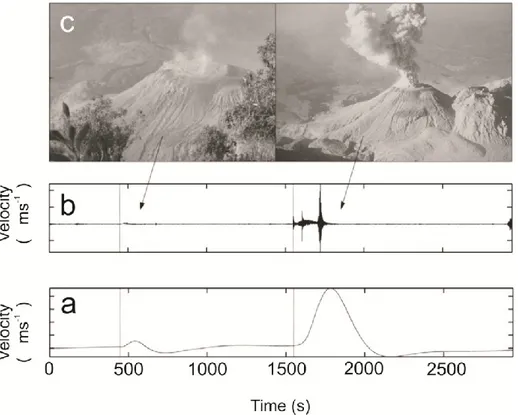
Figure 1.3: a) Band pass filtered (600-30 s) and b) raw signals for VLP events recorded at Santiaguito volcano. Images in c) show the corresponding volcanic activity. Modified from Zobin [2012].

1.2.4 Volcanic tremor

Volcanic tremor is a persistent seismic signal, lasting from several minutes to several days or even months, often preceding or accompanying volcanic eruptions [e.g., Kostantinou and Schlindwein, 2002]. Even if the frequency content may be characteristic of the individual volcano, volcanic tremors are generally characterized by similar frequency content to LP signals, that is roughly 0.5-5 Hz. Furthermore, in some cases, it is possible to identify a fundamental frequency and the relative

9 harmonics; the corresponding signal is called volcanic harmonic tremor. In most cases the wavefield is composed of Rayleigh and Love waves, and it is strongly affected by path effects [e.g., Kostantinou and Schlindwein, 2002], but some studies proved that a mixed composition of both body and surface waves may be dominant at other volcanoes [i.e., Deception Island, Almendros et al., 1997]. According to Kostantinou and Schlindwein (2002), several interpretations of the volcanic tremor source mechanism are possible: for instance, fluid oscillation induced by external causes to the fluid, i.e. like fracturing of the surrounding bedrock and formation of a new feeding branch, or a sudden variation in the fluid supply [St Lawrence and Qamar, 1979; Ferrick et al., 1982]. Aki et al. (1977) proposed that tremor is due to the vibration of a crack chain as the magma ascent to the surface through the network. Chouet [1986, 1988] proposed as a source of tremor the wall vibration of a magma filled crack, due to a pressure disturbance. In hydrothermal area, tremor-like signals are likely to be due to water boiling processes at depth [Kieffer, 1984; Kedar et al., 1996]. Crosson and Bame [1985] found, by realizing a model of a spherical cavity in the hosting rock containing a smaller gas filled cavity, that tremor at Stromboli could be explained as magma resonance in consequence of the expansion of the slug.

It is noteworthy that onset, evolution and conclusion of the summit paroxysmal activity are typically well-correlated with the pattern of the volcanic tremor. However, the relationship between amplitude variations of volcanic tremor and magmatic activity is not univocal. Indeed, in some cases there is a good correlation between the occurrence of the former and the renewal of shallow volcanic activity, as reported for a few volcanoes [e.g. Kilauea, Dvorak and Okamura, 1985; Pavlof, McNutt, 1986; Etna, Cannata et al., 2008]. Alternatively, the variation in amplitude of volcanic tremor may be related to the movement of fluid at great depth and not accompanied by any variation in observable volcanic activity [Aki and Koyanagi, 1981].

1.2.5 Infrasound signals

Acoustic waves are longitudinal waves due to the compression-expansion of the medium in which they propagate, in response to the vibration of the source of sound. For frequencies below 20 Hz, the threshold of hearing of human being, they are called infrasound. Volcanoes radiate acoustic energy mainly in this range of frequencies. Infrasound was first recorded by microbarometers after the violent 1883 eruption of Krakatau [Strachey, 1888], which induced low frequency oscillations that propagated around the Earth several times, as also audible sounds of “heavy

10 gunfire” as far as 5000 km away [Simkin and Fiske, 1983]. Since then, and especially in the last decades, infrasound has become a widespread method of investigation and monitoring of volcanoes. Infrasonic transients (hereafter: infrasonic events) have been frequently recorded. During paroxysmal activity or during intense degassing, the can merge giving rise to an almost continuous signals named infrasonic tremor [Montalto et al., 2010].

Several processes have been recognized as sources of infrasound.

A group of source models for infrasound events deals with phenomena linked to explosions of strombolian bubbles. For instance, Vergniolle et al. [2004] suggest that infrasound is produced from the oscillation of gas slugs prior to the bursting, when they reach the free magma surface. This model will be used to fit some data in the following pages, thus it is worthy to add some more information about it. According to the authors, bubbles reach the surface with some excess pressures. As a consequence, strong volumetric vibration of the bubble wall, (corresponding to a thin layer of magma), pushed by variation of pressure inside the bubble prior to bursting, occur, producing sound. The bubble shape is approximated by a hemispherical head and a cylindrical tail, as expected in slug-flow [Vergniolle et al., 2004]. The propagation of pressure waves is radial and the waveform of the resulting infrasound signal consists of a first energetic part roughly composed of one cycle (or one cycle and a half), corresponding to the bubble vibration, followed by a second part with weaker oscillations [Vergniolle et al., 2004]. The experimental data may be fitted by synthetic waveforms obtained by the equation [Vergniolle and Brandeis, 1996]:

(1)

where the first term is excess pressure in air, t is time, r is the distance source-sensor, c is the sound speed in air, R is the bubble radius and ρair is the air density.

It is worth noting that several parameters are needed to solve this equation: density of magma, thickness of magma above the vibrating bubble, magma viscosity, length of the bubble and initial overpressure [an exhaustive discussion can be found in Vergniolle and Brandeis, 1996]. However, some of them (i.e. viscosity and density of the magma) can be derived from complementary studies. Concerning the thickness of the magma wall, for instance, it is likely to be on the same order of magnitude of the diameter of the ejecta, thus it can be easily inferred [Vergniolle et al., 2004]. Once all the parameters are fixed, we can easily calculate the characteristic features of the bubble (overpressure, length and radius) by equation (1).

11 Another model based on volcanic slugs suggests that very large bubbles are forming at the shallow part of the conduit for coalescence processes. The escape of gas through a tiny hole, that breaks the bubble walls, produces a low monochromatic sound [Vergniolle and Caplan Auerbach, 2004]. Differently, there is a class of models that links infrasound sources with resonance phenomena. Acoustic resonance can be defined as the acoustic response of a contained region to pressure disturbances, a feature of a perturbed sound field interacting with two or more boundaries or fluid discontinuities [Fee et al., 2010a]. Indeed, resonance is due to multiple reflection of pressure disturbances at the boundary of the resonator, and can be defined as a propagation path effect [Garces and McNutt, 1997], which gives us useful information about the geometry and/or the characteristics of the resonator.

Resonance of the shallow portion of the conduit, for instance, have been hypothesized at several volcanoes [i.e., Buckingham and Garces, 1996; Hagerty et al., 2000]. For example, at Kilauea and Villarica were found evidences of a resonant monotonic and long lasting tremor, whose source coincides with skylights above lava tubes [Garces et al., 2003; Matoza et al., 2010a] and central vents [Ripepe et al., 2010].

Such kind of resonance is likely to occur when the ratio between the wavelength and the cavity dimension is comprised between 1/3 to 3 [Fee et al., 2010a; Morse and Ingard, 1968]. For a fluid filled fracture of length L and width W, longitudinal and lateral sets of resonance modes are expected (respectively 2L/n and 2W/n, with n=1,2,3) [De Angelis and McNutt, 2007]. Nevertheless, it is common to observe only longitudinal modes, coherently with the cylindrical shape of the very shallow conduit inferred at many volcanoes. Indeed, for wavelength much longer than the radius of the conduit, lateral modes are negligible, and only the longitudinal modes must be taken into account [Garces and McNutt, 1997].

According to fundamental law for pipe resonance [equation (2); Hagerty et al., 2000]:

(2)

with c equal to the acoustic velocity and f0 fundamental frequency of resonance, while Lr is the

length of the resonator.

However, the type of triggered resonance depends on the boundary conditions. For a resonant pipe with matched boundary condition, thus having both the termination closed or both open, the resulting spectra show integer harmonics of the fundamental. In the opposite case (open-closed termination), odd harmonics of the fundamental will be observed. It is noteworthy that the

12 condition of closure is due to change of the impedance contrast, i.e. cross sectional variations or drastic discontinuity in the magma properties [Garces and McNutt, 1997; De Angelis and McNutt, 2007]. Furthermore, it must be remarked that the observation of an open vent does not imply acoustically open termination, and vice versa [Garces and McNutt, 1997].

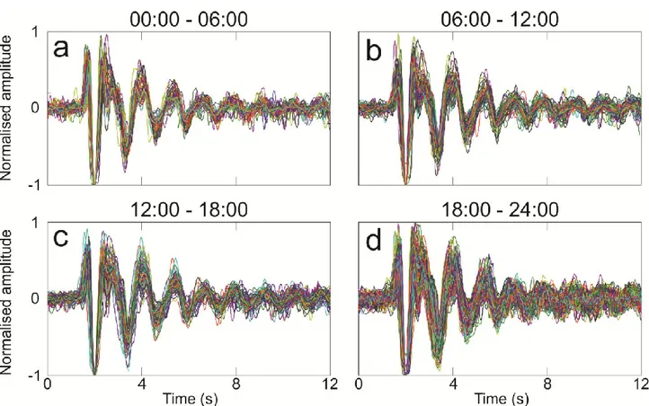
Finally, an end correction must be taken into account when dealing with open vent [Morse and Indegard, 1968]. Indeed, in the near field, the movement backwards and forwards of the air due to the vibration of the surface of the source, adds inertial mass to the vibrating mode, thus affecting the frequency of resonance. For this reason, a term, namely end correction, is introduced to extend the length of an open-ended vibrating column [Rossing, 2007]. For a closed pipe the end correction is zero, while for an open pipe is 0.6*a, with a radius of the pipe [Miklos et al., 2001]. Other possible kinds of resonance have been recognized at active volcanoes [i.e., Goto and Johnson, 2011; Fee et al., 2010a]. When the wavelength is much larger than any dimension of the resonator, harmonic oscillation with only one degree of freedom, i.e. the volume, may occur [Fee et al., 2010]. This kind of resonator is called lumped acoustic element [Kinsler, 1982], and the most common example of it is the Helmholtz resonator. A simple Helmholtz resonator is made up of a cavity connected with the outside space through a narrow neck or through an opening [see Fig.

1.4; Alster, 1972]. The resonator reverberates with a single frequency, computed on the basis of

the following equation [Kinsler et al., 1982]:

(3)

Where S is the area of the neck, V is the volume of the cavity and k’ is the effective length of the neck, provided of end correction by the equation:

(4)

with A and l equal to the radius and length of the neck, respectively.

Indeed, the compressible fluid in the resonator acts like a spring with constant:

(5)

where ρair is the density of the air. The behavior of the fluid in the neck is correspondent to a

lumped acoustic element [Rossing, 2007]. The magnitude of the lumped mass resonator is given by:

13

(6)

Figure 1.4: Simplified scheme showing an Helmholtz resonator. Modified from Rossing [2007].

At Halema’uma’u Crater (Kilauea Volcano), Fee et al. [2010a] inferred the presence of a double resonance mechanism to justify the presence of two spectral bands in both infrasonic tremor and events, namely: “f1” at 0.3-0.6 Hz, and “f2” at 1-3 Hz. Authors claim that the former spectral band is due to Helmholtz resonance of the gas filled cavity beneath the vent, whereas the latter and higher frequency band is due to standing waves of the same cavity (see Fig. 1.5).

Figure 1.5: Cartoon of Halema’uma’u double resonant cavity [Fee et al., 2010].

Obviously, different dynamics may be active at other volcanoes. For example, infrasound may be related to the sudden uncorking of the volcano, when the pressure exceeds the critical threshold releasing acoustic energy. This mechanism is believed to be more common in presence of intermediate viscosity magma, where Vulcanian eruption -disrupting the plug obstructing the conduit- may occur [Johnson and Lees, 2000; Uhira and Takeo, 1994]. Another example of source

14 model in which more violent level of activity is implied is given by the 8 March 2005 Vulcanian eruption of Mt. Helens, for which during the initial emission of gas, quite fast ejection of gas and ash is likely to have occurred [Matoza et al., 2007]. The acoustic signals corresponding to this phase of the eruption were compared to low frequency jet noise, on the basis of a similarity with the physical mechanism of noise radiation from the aircrafts [Matoza et al., 2009a].

Sometimes the occurrence of infrasound may be due to hydrothermal phenomena. For instance, at Mt. St. Helens, from November 2004 to March 2005 the eruption was characterized by repetitive infrasound signals associated to LP events that were probably linked to hydrothermal processes. It was suggested [Matoza et al., 2009b] that the repeated and rapid pressure loss from a hydrothermal crack system caused both acoustic and seismic radiation. Indeed, heated fluid may cause the pressure buildup required to open the crack system. The sudden release of pressure produces a broadband infrasound signal, and, in the meanwhile, induces the crack collapse, thus generating infrasound signals.

Finally, it must be taken into account that also landslides and pyroclastic flows, both common phenomena in volcanoes environment, are able to produce infrasound [Oshima and Maekawa, 2001; Moran et al., 2008a].

1.3 Analytical methods

1.3.1 Transient detection

Detection algorithms are the fundamental first step of every research study or monitoring activity based on continuously recorded signals. Indeed, dealing with big amount of temporal traces requires the use of an automatic algorithm to detect the occurrence of transients. On the base of the characteristics of the investigated signals, and thus on the base of the type of alterations we expect to detect in correspondence of an arrival of a seismic/infrasonic wave, different trigger algorithms can be used. For instance, they can be based either on the time or frequency domain, they can search for a specific expected pattern, or make use of the particle motion or the polarization characteristics of the signal, such as rectilinearity or planarity [Withers et al., 1998]. One of the most extensively used algorithm, named STA/LTA (Short time average/long time

15 [Whiters et al., 1998]. This method requires the definition of two time windows, one relatively shorter than the other. It has been estimated that ideal conditions for the algorithm are given when the two windows are respectively 3 and 27 times the central period of the frequency band of interest [Whiters et al., 1998]. The energy density in each window is computed by using root mean square (hereafter RMS) and then the ratio between the values estimated for the two windows is calculated. Thus, the two windows are simultaneously shifted along the traces, and a transient is detected when the value of such energy density ratio overcomes a fixed threshold. It must be noted that this algorithm tends to produce false arrivals in condition of irregular noise [Havskov and Alguacil, 2004].

Alternatively, an effective trigger algorithm used in this work is the percentile method [for an example see Fig. 1.6; Cannata et al., 2011b].

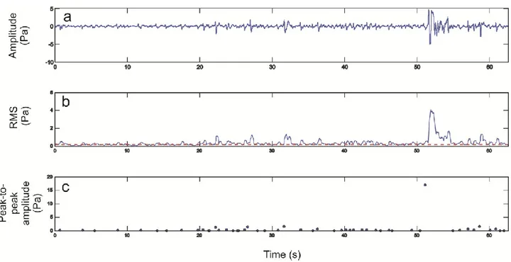
Figure 1.6: Example of percentile trigger analysis applied to moderate puffing activity at Mt. Yasur. a) Raw signal (begin time: July, 7th 2011, 06:01:54). b) RMS envelope of signal shown in a); the red dotted line represents the percentile threshold value. Blue dots in c) represent triggered events.

The RMS envelope is computed by using a sliding window with a fixed duration. Successively, the percentile of RMS envelope is computed by using another moving window. A percentile threshold

ptr is established, as the value for which at most (100 × ptr) per cent of the measurements are less

than this value and 100(1 – ptr) per cent are greater. A transient arrival is detected every time the

RMS percentile overcomes the fixed threshold. This method was found to be more effective than STA/LTA when dealing with closely spaced events [Cannata et al., 2011b].

16

1.3.2 Location analyses

1.3.2.1 Infrasound location

Unlike seismic signals, whose epicentral location errors are generally larger than 100 m, infrasound location can be much more precise [up to 3 m; Johnson, 2005]. This difference depends on several factors. Firstly, considering the lower velocity of acoustic waves in respect of seismic ones, small changes in the source position affect more the infrasound travel and arrival times than in the case of seismic signals [Johnson, 2005]. Secondly, the propagation velocity of the seismic waves [Johnson, 2005; Arrowsmith et al., 2010] is often poor-known and identifying correlated phases for emergent or sustained seismic signals is still difficult [Arrowsmith et al., 2010]. Infrasound location techniques, using semblance or cross correlation functions to compare signals recorded at several sensors, have allowed recognizing active vents in multivent systems such as Stromboli [Ripepe and Marchetti, 2002], Mt. Etna [Cannata et al., 2009a] and Kilauea [Garces et al., 2003]. Different techniques have been developed to locate the infrasound sources [e.g. Ripepe and Marchetti, 2002; Garces et al., 2003; Johnson, 2005; Matoza et al., 2007; Jones et al., 2008; Jones and Johnson, 2010; Montalto et al., 2010]. Among them grid search methods are particularly suited for dense network recordings.

These methods are based on the designation of a grid, spread all over the region of interest for the determination of the source position. For infrasound, it is convenient to define a bi-dimensional grid of assumed source positions coincident with the topography, since the vent radiating infrasound can be considered a source point located on the topography. Successively, the procedure requires to find a source position on the grid that allows for a set of theoretical arrival times (τi, i =1,…, N), that yields maximum value of a similarity function calculated on the N-channel data.

The procedure includes several steps common to other location methods [e.g., Almendros and Chouet, 2003; Ripepe et al., 2007]. In particular, a start time ts is fixed as the time of first arrival at

a reference station (generally chosen on the basis of the highest signal to noise ratio). The source is iteratively assumed to be in each node of the grid, and for each node the origin time is calculated, assuming a certain value of propagation velocity of the infrasonic waves c, as follows:

17 where r is the distance between the reference station and the node of the grid assumed as source location. The theoretical travel times are calculated at all the sensors ti (i =1,…, N, number of

stations):

(8)

where ri is the distance between the station i-th and the node of the grid assumed as source

location. Then, using these theoretical travel times and the origin time, signals at the different stations are delayed and a function is applied in order to compare the windows of signals obtained and define the level of similarity among them. The source coincides with the point of the grid where the maximum of such function is observed.

Two functions have been used in this work, the semblance function [Neidel and Tarner, 1971] and the brightness function [Kao and Shan, 2004]. In some cases, in order to obtain high precision location, the two functions were also combined together [Cannata et al., 2011a].

Let us consider traces U, acquired by a certain number of sensors N; the semblance is defined as [Neidel and Tarner, 1971; Almendros and Chouet, 2003]:

(9)

where Δt is the sampling interval, τi is the origin time of the window sampling the i-th trace,

Ui(τi+jΔt) is the j-th time sample of the i-th U trace, and M represents the number of samples in

the window. S is a number between 0 and 1. The value 1 is only reached when the signals are identical, not only in waveform but also in amplitude. Eventually, in order to make S values unrelated to the different amplitudes of the signals recorded at distinct stations, it is useful to normalize the waveforms dividing each trace by its maximum absolute value. Indeed, as also argued by Almendros and Chouet [2003], the semblance location technique is mainly based on the quantification of the similarity among waveforms recorded at different stations, and then we are not interested in the relative differences in amplitudes. However, when many stations, located at very different distances from the source, are used, it can be useful not to normalize the amplitudes before calculating the semblance values. Thus, greater “weight” is given to the stations nearest to the source and characterized by the highest signal to noise ratio [Cannata et al., 2009c]

The definition of brightness was given by Kao and Shan [2004], and was used to map the space distribution of seismic sources by the so-called Source-Scanning Algorithm. Here we use the following slightly modified brightness definition:

18

(10)

where Wi is a time window of the signal Ui multiplied by a hanning window:

(11)

with j =1,…,M. Even in this case the signals Ui have to be normalized such that, if all the largest

amplitudes are aligned at the centre of the considered time windows, B is equal to 1.

In Fig. 1.7 is shown the space distributions of both semblance and brightness values for the same event. Both the advantages and disadvantages of each method are evident in the picture. For instance, the drawback of the semblance distribution is the presence of pronounced lobes extending over almost the whole grid, giving rise to many relative maxima. On the other hand, the drawback of the brightness distribution is the wide area characterized by high brightness values that does not allow locating the source precisely.

The joint semblance-brightness distribution [Cannata et al., 2011a] overcomes the drawbacks of both the methods. Indeed, once the space distributions of both semblance and brightness values are determined, the two grids of values are normalized, by subtracting the minimum value and dividing by the maximum one. Thus, the values belonging to two grids range from 0 to 1, and the same weights are assigned to semblance and brightness. Then, the two normalized grids are summed node by node. The source is finally located in the node where the delayed signals show the largest composite semblance brightness value. This joint method not only shows the high location resolution of the semblance method, but also, by the brightness function, strongly reduces the side lobes characterizing semblance locations [Jones and Johnson, 2010; Montalto et al., 2010].

19

Figure 1.7. Example of semblance, brightness and semblance+brightness space distribution for an infrasound event generated by the eruptive fissure. The concentric lines in the top plots are the altitude contour lines from 3 to 3.3 km a.s.l.

1.3.2.2 Seismic tremor location

As previously said, volcanic tremor is a continuous or long-lasting signal for which no method based on the inversion of the travel time could be used. For this reason, the localizations of volcanic tremor are usually based on the spatial distribution of the amplitudes at all the stations of the network, the so called amplitude decay method, which takes into account the expected amplitude decay through the path source/station [e.g., Battaglia et al., 2005; Di Grazia et al., 2006; Patanè et al., 2008].

Thus, according to these methods, the first step is the definition of a 3D grid, whose nodes are iteratively assumed coincident with the source of tremor. Indeed, fixing a node as the source, a distribution of expected amplitude of the signal is computed at each station. The decay in amplitude during the travel path is computed by the following general law:

(12)

where f is the frequency, s the distance, b is the exponent, which takes values of 0.5 or 1 for the cases of surface and body waves, respectively, A0 the initial amplitude at frequency f, A the

amplitude at frequency f and distance s, and α, the frequency dependent absorption coefficient, given by:

20

(13)

with c corresponding to the wave velocity and Q equal to the quality factor, indicating the loss of energy during each cycle of the wave, and quantified with the following equation [Knopoff, 1964]:

(14)

where E is equal to the peak energy reached in each cycle, and ΔE is the energy loss in same cycle. The equation (12) can be linearized in the following form:

(15)

where a (lnA0) and b are constant, Ai is the amplitude at the station ith, and si is the distance

source–station ith. The RMS value is used for quantifying the amplitude of the volcanic tremor. The location of the source is found by evaluating the goodness of the regression fit between the theoretical and the experimental amplitude (R2), as the amount of variance explained by the linear fit with respect to the total variance of logA(s) [Di Grazia et al., 2006]. Finally, the position of the source is found as the centroid of the 3D points whose R2 does not differ more than 1 % from the maximum R2.

Even though the frequency dependent absorption coefficient does not affect excessively the source location [Battaglia et al., 2005], it must be estimated in order to apply the method. At Mt. Etna it was evaluated by systematically attributing different values to α, and then searching for the best values achieved for R2. Thus, values comprised between 0 and 0.2 were obtained for α [Patané et al., 2008].

1.3.2.3 LP events location

LP events in this work were located by combining together two location methods above described: semblance and amplitude decay (Neidel and Tuner, 1971; Battaglia et al., 2005). Indeed, as in the previous case a grid is defined, and then each node of the grid is iteratively assumed to be the source. Successively, both semblance and amplitude decay functions are computed. Thus, the source is located where is the maximum of the two combined function.

21

1.3.3 Spectral analyses

In order to investigate the characteristics of a temporal series in the frequency domain it is necessary to apply different spectral analyses methods. Basically, a spectral analysis is the conversion of signals, made up of sinusoids in the time domain, into spectral peaks in the frequency domain [Hasada et al., 2001]. In the present thesis two spectral analysis methods have been applied: FFT analysis and Sompi method.

1.3.3.1 FFT analysis and pseudospectrograms

The most common way to perform a signal de-convolution into the frequency domain is the Fourier analysis. Indeed, signals characterized by periodicity can be projected into the mathematical base of the Fourier series, thus into a sum of sinusoidal components. However, this kind of mathematical process is not valid for not periodic signals, such as short-time lasting transient. Therefore, in order to achieve information about the weight of each frequency component in a given transient signal x, we need to apply the Fourier Transform, given by:

(16)

with f frequency and t time, X(f) is the signal in the frequency domain while x(t) is the signal in the time domain, and i is equal to . The opposite mathematical operation is called Fourier anti-transform, and it is used to express in the time domain a frequency based signal.

As we are commonly dealing not with continuous signal, but rather with temporal series sampling the physical phenomenon at a given interval of time, the Fourier transform is defined Discrete Fourier Transform (DFT) and it is applied only to the portion of signal investigated.

The fastest way to solve a Discrete Fourier Transform is by using the Fast Fourier Transform (FFT) algorithm [Cooley and Turkey, 1965]. The N point signal is divided in N signals with one point each, then the spectrum is computed, and finally all the spectra obtained are averaged [Smith, 1999]. The data obtained can be represented in different ways. One of the most extensive representations, particularly useful when dealing with big amount of data -for instance in order to identify spectral variation through time- is the spectrogram. It is obtained by putting each

22 spectrum near to the other along x-axis and representing frequency along the y axis and spectral amplitude as color shading. However, in this thesis extensive use of pseudospectrograms (an example in Fig. 1.8) was made, thus it is worthy to spend some words about this.

Figure 1.8: a) Normalized pseudospectrogram of the so called Mixed- Events (MX) recorded at the vertical component of IVCR station, at Volcano (Sicily). Each spectrum was calculated by averaging the spectra of the MX events occurring during 10-days long interval. The black rectangles, located inside the plot, show time intervals with no MX events. The top empty rectangles and roman numbers indicate the periods characterized by the seismic sequences; b) and c) Peak frequency and quality factor of the vertical component of the seismic signal of IVCR station, obtained by Sompi method for autoregressive (AR) orders ranging between 4 and 60 (see section 1.3.3.2. for details) . From [Alparone et al., 2010].

Indeed, since for many volcanoes infrasound events are discrete transients lasting from a few seconds to tens of seconds and occurring tens of seconds to hours, and occasionally days, apart, the classic representations of FFT analysis (i.e. the spectrograms) would mainly be made up of noise spectra (mostly wind noise), that would hide the spectral features of infrasound events related to volcano activity. In light of this, in place of classic spectrograms, pseudospectrograms were drawn as follows. For each event a spectrum is calculated. Next, to maintain the temporal information, an averaging process of the spectra, falling in sliding time windows, was performed. The duration of such sliding windows is a critical factor, since it must be a compromise between the need for detailed time information (short time interval), and continuity in the representation

23 that takes into consideration the occurrence rate of infrasound events (long time interval). Each averaged spectra is gathered as column in a single matrix, arranged in temporal order. This matrix was visualised as a pseudospectrogram. Hence, in the x-axis the time is reported, the y-axis represents the frequency and the colour scale shows the spectral amplitude. In order to gather the most complete information, it is useful to produce pseudospectrograms using both normalized averaged spectra and the original spectra, as non-normalized spectra will be dominated by high-amplitude phenomena that obscure the spectral content of low high-amplitude events. In the normalized pseudospectrogram the latter information is preserved, but, on the other hand, the information on the amplitude of observed phenomena is lost. It is noteworthy that pseudospectrograms, even if differently named, have been used several times in literature to analyze group of “discrete” seismic and acoustic signals [e.g., Saccorotti et al., 2007; Molina et al., 2008; Moran et al., 2008b; Di Grazia et al., 2009; Alparone et al., 2010].

1.3.3.2 Sompi analysis

The FFT algorithm it is not suited for really short time signal. In fact, the resolution in the frequency domain depends on the length of the time window applied to the signal. Furthermore, the decomposition of the signal in harmonic components is not really representative of signals growing or decaying in time, like in presence of energy dissipation or supply, where the frequency must be defined in the complex rather than real frequency domain.

An alternative procedure to acquire information on the signal in the frequency domain is the Sompi method [Hori et al., 1989; Kumazawa et al., 1990] . According to this method, the temporal series is de-convolved into a linear combination of a finite number of sinusoidal wave-elements. The latter are defined by two complex numbers, z and α, defined as (Kumazawa et al., 1990):

(17)

where are zand ωz are respectively the real and imaginary part of the complex angular frequency,

and:

(18)

with Az and θ, real amplitude and phase at the origin time. The ordinary frequency f and the

24

(19)

(20)

while the quality factor is [O’Connell e Budiansky, 1978]:

(21)

where a smaller value of Q corresponds to major losses of energy during each oscillation. The general law for the amplitude decay is given by [Kumazawa et al., 1990]:

(22)

where m represents the number of wave-element in which the signal is decomposed, and is defined as the order of the regression mode. The choice of the order is fundamental because it defines the number of elements in which the signal must be decomposed. Many authors use a wide range of orders to discriminate coherent elements (i.e., Kumagai et al., 2005; De Angelis and McNutt, 2005)

In the Fig. 1.9, an example of Sompi analysis in the bidimensional plane frequency - growth rate is shown. All the scattered points represent incoherent noise, whereas the densely populated lines, that remain stable when the order of the regression order changes, are resolved dominant modes [Hori et al., 1989].Another example of Sompi analysis is given in Fig. 1.8.

25

Figure 1.9: Example of Sompi analyses. The two signals at the top, respectively an LP event from Kusatsu-Shirane and from Galeras, are analyzed below by Sompi method. Indeed, the two graphs below plot the complex frequency of individual wave element versus growth rate for all the performed autoregressive order (AR) trial (20 to 60). The solid lines represent couple of points with same value of Q. Dominant modes are highlighted by circles. Modified from Kumagai and Chouet (1999).

1.3.4 Cross-correlation

In order to identify pattern in the huge amount of seismic/infrasonic signals that accompany an eruption, signal classification methods are required. Indeed, acoustic or seismic events are commonly grouped on the basis of their frequency content. Nevertheless, much information could be achieved by comparing waveforms, which can be grouped into clusters with a physical meaning.

In order to do that, a time window of fixed length is extracted from the signal. Then, all the events are compared by using the following cross-correlation function:

26 with xi ith sample of the signal x, yi-l is the (i-l)th sample of the signal y, n is the number of events

to be compared, and the over-bar represents the mean value of the signal [Green, 2005]. The relative position of the two windows of signal is expressed by the lag l. A value of cross correlation coefficient equal to 1 means that the signals are identical, whereas -1 stands for opposite

signals, and 0 for total absence of correlation. Using this function, each event is cross-correlated with the other.

Successively, a matrix, with size n x n, is realized by plotting the maximum correlation coefficient. For instance, a generic value mxy of the matrix represents the maximum correlation coefficient

obtained for signals x and y, for different trial lags [Green and Neuberg, 2006].

In order to detect families of events from the matrix, a coefficient threshold is established. A “master event” is selected as the event with the biggest number of threshold excesses. Then, there are mainly two procedures to obtain individual families:

 Bridging technique [e.g., Barani et al., 2007]: All the events with , in respect of the

master event, over the threshold are grouped into the same family and removed from the dataset. Secondly, all the events with , in respect of the removed events, over the fixed

threshold, are grouped in the same family, independently from their similarity to the master event. The procedure is completed when all the possible families are grouped.  Green and Neuberg method [Green and Neuberg, 2006]: An average waveform is obtained

by stacking all the events with in respect to the master event- over the threshold. Then

the cross-correlation values are computed again in reference to the stacked event, and all the events that overcome the fixed threshold are grouped as a family and removed from the dataset. Even in this case, the procedure is completed when all the possible families are grouped.

1.3.5 Seismo-acoustic energy partitioning

The evaluation of the partition between seismic and acoustic energy during volcanic eruptions has proven to be really useful in order to acquire information about the dynamics active at different volcanoes [i.e., Johnson and Aster, 2005] and at the same volcano during different episodes [i.e. Sahetapy-Engel et al., 2008]. Estimations of elastic energies of acoustic and seismic wave field can

27 be useful in order to infer physical constraints about the eruptive mechanisms and to provide quantitative information about condition and intensity of the eruption [Johnson and Aster, 2005]. Seismo-acoustic partition is computed from seismic and infrasonic traces by calculating individually the energy radiated from the source in the acoustic and in the seismic field, and then successively their ratio, namely VASR (Volcano acoustic seismic ratio; Johnson and Aster, 2005). The total acoustic energy radiated into the atmosphere can be estimated by integrating in space and time, over an hemi-spherical surface, the energy density, which is proportional to the square of the excess pressure ΔP [Johnson and Aster, 2005; Firstov and Kravchenko, 1996; Johnson, 2003; Vergniolle et al., 2004]:

(24)

with r distance source-station, ρair and cair respectively air density and sound speed in the air.

Equation (24) requires the assumptions of linear propagation and isotropic travel path of the acoustic wave through the atmosphere. The first statement is verified for moderate explosions, with VEI smaller than 2 [Johnson and Aster, 2005]. The assumption of isotropy of the travel path, instead, is a valid only if the recording stations are located at few kilometers of distance from the source. Bias, due to the noise produced by high intensity winds and/or eventual limitations related to the instrumental response, must be taken into account when evaluating the radiated energy from the recorded signal.

Seismic energy can be estimated through the following equation [Johnson and Aster, 2005; Boatwright, 1980]:

(25)

where ρearth and cearth are respectively density and P wave velocity into the volcanic edifice, A is the

attenuation due to intrinsic and scattering dissipation and S is the site response. Equation (25) assumes that the dominant wave field is made up of pure body waves propagating with a single velocity toward the station. Furthermore, the radiation is considered isotropic and the attenuation negligible. The validity of these assumption, have already been verified at several volcanoes [Etna; Sciotto et al., 2013; Karymsky and Erebus; Johnson and Aster, 2005]. Nevertheless, the application of the equation, require verifying them for the specific studied volcano.

28

(26)

The VASR parameter is basically an indicator of the coupling among the source, the surrounding medium and the atmosphere. Good coupling with the atmosphere is favored by low density of eruptive plumes, or from the absence of a cap rock plugging the conduit. Similarly, the energy associated to seismic waves, traveling inside rock medium from the source to the station, is affected by conduit conditions (e.g., explosive source depth, conduit width) as well as intrinsic attenuation and scattering [Andronico et al., 2013].

29

Chapter 2: Insights into Mt. Etna shallow

conduit dynamics

30

2.1 Mt. Etna: an introduction

2.1.1 Geographical and tectonic setting

Mt. Etna is a Quaternary stratovolcano, characterized by Na-alkaline magmatism [e.g., Cristofolini and Romano, 1982]. It is located on the eastern coast of Sicily, nestled into a peculiar convergence of tectonic elements. Indeed, it lies at the front of the collision belt (Apenninic-Maghrebian Orogen) -developed at the margin of the Africa promontory- and at termination of the Malta Escarpment fault, a Mesozoic discontinuity separating the continental crust of the Pelagian Block [Barreca et al., 2012; Burollet et al., 1978] from the oceanic crust of the Ionian See [Makris et al., 1986; Monaco et al., 2005]. Such characteristic position reflects on the complexity of the structural elements affecting the volcano (see Fig. 2.1). Indeed, the eastern flank is characterized from the presence of a normal fault system, with direction SSW-NNE in the north-eastern sector of the volcano, and NNW-SSE toward south-east, where a slight right lateral component of motion was inferred [Monaco et al., 1995, 1997, 2005; Lanzafame et al., 1996; Azzaro, 1999]. Most of the segment faults are accompanied at the surface by steep slopes called “Timpe”, with Late Pleistocene to Holocene vertical slips ranging from 1 to 2 mm/y [Monaco et al., 1997]. A shallow level (<3) seismicity, with M <4.5 is associated to this system [Azzaro et al., 2000]. The southernmost termination extends offshore at the base of the Malta Escarpment fault [Monaco et al., 1995]. According to some authors, the northward prosecution of the system corresponds to the Tindari-Letojanni system, which marks the alignment of the islands Salina, Lipari and Vulcano [Ghisetti, 1979; Continisio et al., 1997; Lanzafame and Bousquet, 1997].

31 

Figure 2.1: Geological sketch-map of the Mt. Etna region. Key: (1) Alluvial deposits ; (2) Late Wurmian alluvial fan; (3) Trifoglietto, Ancient and Recent Mongibello lava flows (80 ka to Present); (4) Ancient Alkaline Centres lava flows (180-100 ka); (5) Sub-alkaline lava flows (580-250 ka); (6) Middle-Upper Pleistocene foredeep sequences ; (7) Units of the Apenninic-Maghrebian collisionbelt; (8) Hyblean Plateau sequences; (9) Front of the buried Gela Nappe; (10) Major thrust-ramp; (11) Strike-slip fault; (12) Late Quaternary normal fault of the ‘Siculo-Calabrian Rift Zone ; (13) Plio-Pleistocene normal fault; (14) Dry and eruptive fissures; (15) Ms7 earthquakes since AD 1000.From Catalano et al., [2004].

Another fundamental tectonic structure, whose movement is deeply connected to the volcanic activity, is the Pernicana Fault: one of the most active fault systems of Mt. Etna. It is located in the NE sector of the volcano edifice with strike E-W, and it extends from the North East Rift until the coastline, with a total length of 18 km [Neri et al., 2004]. Along the Pernicana fault the motion

32 changes from normal dip-slip at the westernmost termination to the left-strike slip motion at the eastern one [Azzaro et al., 2001]. Jointly with the NNW-SSE Rift, it is believed to accommodate, on the summit area and on the NE rift, the extension, related to the regional tectonic contest, [Monaco et al., 1997; 2005]. Furthermore, together with the Mascalucia-Tremestieri-Trecastagni fault system –characterized by strike NNW, right lateral movement and superficial seismicity- delimitates the boundaries of an unstable edifice sector, with movement toward ESE.

Extensional features affect also the summit area of the volcano edifice, where these tectonic elements are deeply linked to the major magma feeding system [Catalano et al., 2004]. Indeed, Mt. Etna summit area is marked by the presence of three rifts, known as NE, NNW-SSE, and N-S rifts. The former is an eruptive fissures network with strike 42-47°C and with dispersion axes comprised between 15-62°C [Branca et al., 2003]. The second rift is comprised between the South East Crater and the south-western rim of the Valle del Bove, and shows an overall geometry NNW-SSE, implying a right-lateral component of motion [Monaco et al., 1997, 2005]. Finally, the N-S rift, in the southern slope of the volcano, consists of a series of N-S, to SSW-NNE striking fissures extending for a total length of 10 km.

The first evidences of volcanic activity in the etnean area are dated 500-700 ka, and they are mainly tholeitic/transitional products, likely linked to fissural activity, emplaced in the pre-etnean Gulf (nowadays correspondent to emerged land). The successive phase was characterized by the presence of the so called ancient alkaline center (150-80 ka), which marked a sharp change in the eruptive style and in the composition of the volcanic products. Successively, activity focused in the area of the Valle del Bove, where actually it is possible to see the traces of the different eruptive centers that succeeded in time in the exposed valley rock walls. The stratigraphical sequence is according with a movement of the eruptive center westward through time [Doglioni et al., 2001]. However, since 35 ka, the activity has been persistently occurring at the eruptive center of Mongibello that accounts for one third of the total volume of Mt. Etna [Giacomelli and Pesaresi, 2003]. The history of Mongibello is commonly split in two parts by the occurrence of a violent episode, 14 ka, that led to the formation of a caldera, named “Caldera dell’Ellittico”. Such depression has been filled through time, and above it, a new central summit cone developed and it is actually the theatre of eruptive activity at the volcano.

The summit area of Mt. Etna is currently made up of four active craters: Voragine, Bocca Nuova, South East Crater and North East Crater (hereafter referred to as VOR, BN, SEC and NEC, respectively, Fig. 2.2). Indeed, at the beginning of the century the summit area was characterized

33 by the presence of a Central Crater, filled by the almost not interrupted eruptions [Patanè et al., 2004]. VOR developed in the North-east sector of the summit chasm in 1945 and, successively, a new crateric depression, corresponding to new-born BN, formed and enlarged in the Central Crater. The NEC, instead, developed in 1911 as a pit depression decentred in respect of the Central Cone, and grew up in time reaching lately the maximum altitude of the volcano, since nowadays. Also SEC developed initially as a simple pit crater, in 1971. Its activity increased drastically after 1978, leading to the development of the actual cone. Furthermore, during 2011-2013 a large new pyroclastic cone, named “New South East Crater”, formed on south-east flank of SEC [Patanè et al., 2013].

Figure 2.2. Digital elevation model of Mt. Etna with the eruptive fissure opened on 13 May 2008 (thick black line “EF”). The digital elevation model in the upper left corner shows the distribution of the four summit.

Volcanic activity may be divided into activity at the summit craters and flank eruptions. The former is characterized by phases of degassing alternating with mild Strombolian activity, occasionally fire fountains, and lava overflows [e.g., Cannata et al., 2008]. In contrast, flank eruptions occur from lateral vents, which are usually located along fracture systems and often related to regional tectonics [e.g., Monaco et al., 2005].