AT RIVER BASIN AND REGIONAL SCALE
:
APPLICATION IN
S
ICILY
DISSERTATION
Submitted in partial satisfaction of the requirements for the degree of
DOCTOR OF PHILOSOPHY
in
HYDRAULIC ENGINEERING
OFFICE OF GRADUATE STUDIESof the
UNIVERSITY OF CATANIA, ITALY
in collaboration with
INSTITUTE NATIONAL DES SCIENCES APPLIQUÉES DE LYON,
FRANCE
Tesi per il conseguimento del titolo Catania, Dicembre 2012
IN INGEGNERIA IDRAULICA
XXIV Ciclo
COMMISSIONE EUROPEA FONDO SOCIALE EUROPEOM
ONITORING DROUGHT
AT RIVER BASIN AND REGIONAL
SCALE
:
APPLICATION IN
S
ICILY
Antonio CASTANO
Tutor:
Prof. Ing. Antonino CANCELLIERE
Coordinatore del Dottorato: Prof. Ing. Giuseppe PEZZINGA
UNIVERSITÀ DI CATANIA Dipartimento di Ingegneria
Civile e Ambientale
Institute National des Sciences Appliquèes
(INSA) de Lyon Sede consorziata:
Thousands have lived without love,
Not one without water
(W.H. Auden)Laudato si’, mi’ Signore, per sor’aqua,
la quale è multo utile et humile
et pretiosa et casta.
(San Francesco d’Assisi)Water is life's matter, matrix, mother, and medium.
There is no life without water.
CONTENTS
1 INTRODUCTION ... 1.1
1.1 BACKGROUND ... 1.1
1.2 RESEARCH OBJECTIVES ... 1.3
2 DROUGHT CHARACTERIZATION AND MONITORING ... 2.5
2.1 DEFINITION OF DROUGHT ... 2.5
2.2 REVIEW OF MAIN DROUGHT INDICES ... 2.7
2.2.1 Meteorological drought indices ... 2.9 2.2.2 Hydrological drought indices ... 2.15 2.2.3 Agricultural drought indices ... 2.18 2.2.4 Operational indices ... 2.18
2.3 CALCULATION OF INDICES AND DROUGHT CLASSIFICATION ... 2.19
2.4 CRITICISM OF EXISTENT DROUGHT INDICES ... 2.21
2.5 ABOUT AREAL EXTENT OF DROUGHT ... 2.25
3 METHODOLOGIES OF DROUGHT ANALYSIS AT DIFFERENT SPATIAL SCALES 3.27
3.1 INTRODUCTION ... 3.27
3.2 COMPARING METHODS OF IDENTIFIED DROUGHTS ... 3.28
3.2.1 Overview ... 3.28 3.2.2 Correlation and concordance analysis ... 3.29
3.3 AGGREGATION OF DROUGHT INDICES AT RIVER BASIN SCALE ... 3.32
3.3.1 Overview ... 3.32 3.3.2 A multidimensional drought analysis ... 3.33
3.4 PROBABILISTIC CHARACTERIZATION OF DROUGHT AREAL EXTENT BASED ON SPI ... 3.36
3.4.1 Overview ... 3.36 3.4.2 Analysis of areal drought extent ... 3.37
4 INVESTIGATED AREAS AND AVAILABLE DATA ... 4.41
4.1 INTRODUCTION ... 4.41
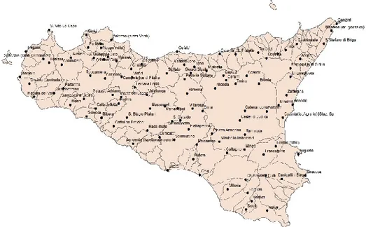
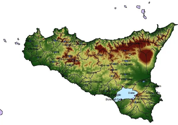
4.2 LOCALIZATION AND GEOGRAPHY OF SICILY... 4.41
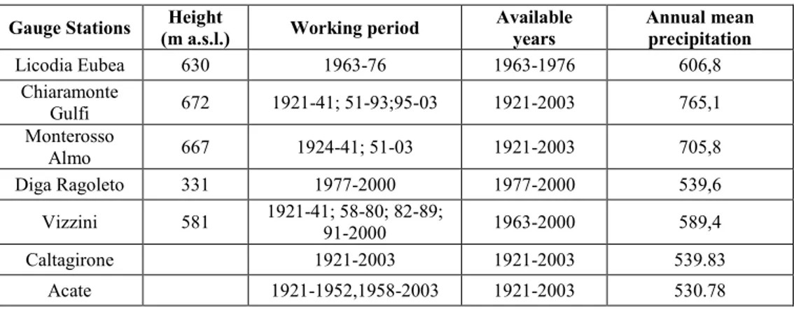
4.3 THE GAUGE STATIONS NETWORK IN SICILY ... 4.43
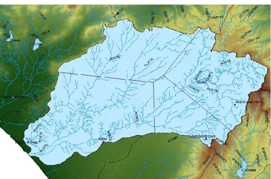
4.4 THE ACATE RIVER BASIN ... 4.47
4.4.1 Localization ... 4.47 4.4.2 Available data in gauged stations ... 4.48
5 COMPARISON OF DROUGHT INDICES ... 5.55
5.1 INTRODUCTION ... 5.55
5.2 COMPUTING SELECTED DROUGHT INDICES ... 5.55
5.2.1 SPI and SSI indices ... 5.56 5.2.2 The Palmer Drought Index ... 5.59
5.3 CORRELATION ANALYSIS OF INDICES ... 5.61
5.4 CONCORDANCE ANALYSIS OF DETECTED DROUGHT PERIODS ... 5.67
6 CASE STUDY: APPLICATION OF AN AGGREGATE INDICATOR TO THE ACATE
RIVER WATERSHED ... 6.69
6.1 INTRODUCTION ... 6.69
6.2 OPERATIONAL COMPUTATION OF ADI ... 6.69
6.3 COMPARISON OF CHARACTERISTICS OF DETECTED DROUGHT PERIODS ... 6.74
7 CASE STUDY: CHARACTERIZATION OF DROUGHT AREAL EXTENT IN SICILY . 7.79
7.1 INTRODUCTION ... 7.79
7.2 PROBABILISTIC CHARACTERIZATION OF AREAL EXTENT ... 7.79
8 CONCLUSIONS ... 8.89
ACKNOWLEDGEMENTS (IN ITALIAN) ... 8.91 LIST OF FIGURES ... 8.92 LIST OF TABLES ... 8.94 REFERENCES ... 8.95 APPENDIX ... 8.103
ABSTRACT
The subject of the dissertation is the investigation of drought features, focusing especially to the characterization and monitoring of droughts at different spatial dimension.
Drought is a natural phenomenon, which presents spatial and temporal features whose knowledge is fundamental for a correct water resources management. Proper definition of droughts and quantification of its characteristics is essential for improving drought preparedness and for reducing its impacts.
Design of mitigation strategies to cope with drought is essential to alleviate many economic, social and environmental problems in different parts of the world and in Europe, particularly in the Mediterranean region (Iglesias et al., 2007; Rossi and Cancelliere, 2012).
Understanding space and time variability of droughts is fundamental for a wide range of water management problems. In order to achieve these goals, the need of appropriate indices oriented to support the analysis and monitoring of such extreme natural phenomenon throughout a multidimensional approach is required.
The multi facets nature of drought requires to assess the capabilities of monitoring indices to grasp different aspects related to the phenomenon. Also, the need arises to aggregate the information from different indices in order to simplify the assessment of drought conditions by decision makers, especially at river basin scale. On the other hand, at regional scale, assessment of the spatial features of drought in terms of areal extent is a prerequisite for a proper identification of appropriate mitigation strategies
The present thesis has addressed some of the above issue, attempting to contribute to a better drought monitoring at river basin and regional scale.
As first step, a methodology of analysis and comparison of most common drought indices has been applied. More specifically, a comparison between the Standardized Precipitation Index, the Standardized Streamflow Index, and the Palmer index has been carried out with reference to the Acate River watershed, in
the south of Sicily. Such comparison has revealed that the three indices present different degrees of agreement in detecting drought conditions depending on the adopted aggregation time scale. Furthermore the analysis has revealed that the SPI at a proper aggregation time scale can be representative of hydrological and agricultural droughts, thus confirming its suitability as a tool for monitoring droughts at river basin scale.
Then a methodology for the aggregation of such indices in a unique one based on Principal Component Analysis has been applied. The resulting index was able to clearly detect most of registered historical droughts; furthermore, the indirect presence of various components of the hydrologic cycle (precipitation, air temperature, streamflow) let the indicator have a lower sensitivity to the variability of a single hydrologic variable. The main advantage of the proposed aggregated index is that it integrates in a single value different information related to meteorological, hydrological, and agricultural droughts.
A methodology for the probabilistic characterization of drought areal extent based on SPI has been developed as a tool to support drought monitoring at regional scale. It consists in the estimation of the measure of drought severity associated with different areal extents (in terms of percentage area of the investigated region). Then a probability distribution has been fitted to drought severity series for different areal extents and drought Severity Area Frequency curves for the region of Sicily have been developed.
Comparison of the developed SAF curves with severity-area curves related to historical droughts, as well as to wet periods, has indicated the feasibility of the developed tool, both to characterize past droughts, as well as to probabilistically assess the magnitude of an ongoing drought for monitoring purposes.
CHAPTER 1
1 I
NTRODUCTION1.1 Background
The latest World Water Development Reports (UN-Water, 2009, 2012) reminds the key role played by water for the whole economic system. Water is not just essential for human life, but also in achieving sustainable development objectives and therefore water availability can be one of the limiting factors for economic and social development. Droughts, being a temporary reduction of precipitation that propagates along the hydrological cycle causing severe water shortages, can therefore have catastrophic impacts especially in those regions already affected by water scarcity.
Europe and the entire Mediterranean area have suffered major droughts in recent years (Zaidman et al. 2001; Lloyd-Hughes and Saunders 2002; Fink et al. 2004; Hannaford et al. 2011; Bonaccorso et al., 2012). Other areas of the world are also experiencing drought conditions, such as continental USA and India, where the 2012 drought has been one of the worst in the last century.
Drought is a natural phenomenon, which presents spatial and temporal features whose knowledge is fundamental for a correct water resources management. Proper definition of droughts and quantification of its characteristics is essential for improving drought preparedness and for reducing its impacts. Furthermore, drought analysis and mitigation have gained further attention by the international scientific community also in light of new scenarios caused by potential trends in climate. It is expected that the intensity and frequency of droughts are going to increase in the future due to climate modifications with a considerable enhancement in inter-annual variability, associated with higher risks of heat waves and decreasing of precipitation, causing droughts as already experienced in recent years (IPCC, 2007).
Many authors have defined the drought concept (Yevjevich, 1967; Dracup et al., 1980; Yevjevich et al., 1983, Rossi et al. 1992; Wilhite, 2000); In general terms, a distinction is generally accepted among different drought related concepts: aridity indicates a natural and permanent climatic condition of low annual
or seasonal rainfall;
desertification identifies a permanent and often irreversible process of decrease or destruction of biological eco-system due to anthropic reasons or climate change effects;
drought refers to a temporary natural condition of a consistent reduction of water availability with respect to long term average condition, spanning over a significant period of time and affecting a wide region.
water shortage is a temporary deficit in the water balance between available resources and demand. It differs from water scarcity which is a permanent condition of insufficient water resources;
Further in this way, can be useful the following Table 1.I where is highlighted the distinction among water deficit phenomena based on their causes:
Table 1.I - Key elements for the definition of water scarcity and drought Timescale
Short-term (days, weeks)
Mid-term (weeks, months, seasons, years)
Long-term (decades)
Cau
ses Natural Dry Spell Drought Aridity
Anthropic Water stress Water scarcity Desertification
Alternatively drought can be defined as an extreme hydro-meteorological phenomenon originated by meteorological anomalies that reduce precipitation thus affecting the state of the various components of the hydrologic cycle (Wilhite, 2000).
In spite of its basic nature of natural hazard, drought should also be considered a man-affected phenomenon (Rossi, 2000). Indeed, this is related to the perception of drought as a harmful phenomenon only where a human community exists and therefore its impacts can be very different according to the level of withdrawals with respect to the available water resources (Rossi et al., 2003). Furthermore, a drought of fixed duration and severity could produce a wide range of consequences according to the level of vulnerability of the water system (Cancelliere et al., 1998).
Design of mitigation strategies to cope with drought is essential to alleviate many economic, social and environmental problems in different parts of the world and in Europe, particularly in the Mediterranean region (Iglesias et al., 2007; Rossi and Cancelliere, 2012).
The ever-increasing demand on water resources calls for better management of the water deficit condition to avoid deficiency in the water supply systems. The consequences of droughts are felt most keenly in areas which are in any case arid (Beran and Rodier, 1985).
Understanding space and time variability of droughts is fundamental for a wide range of water management problems. In order to achieve these goals, the need of appropriate indices oriented to support the analysis and monitoring of such extreme natural phenomenon throughout a multidimensional approach is required.
The multi facets nature of drought requires to assess the capabilities of monitoring indices to grasp different aspects related to the phenomenon. Also, the need arises to aggregate the information from different indices in order to simplify the assessment of drought conditions by decision makers, especially at river basin scale. On the other hand, at regional scale, assessment of the spatial features of drought in terms of areal extent is a prerequisite for a proper identification of appropriate mitigation strategies.
1.2 Research objectives
It is largely recognized that an effective mitigation of the most adverse drought impacts is possible, as long as a drought monitoring is in place able to promptly warn about the onset drought and to follow its evolution in space and time (Rossi, 2003).
During last decades several methodologies for the identification and monitoring of drought events have been developed; more recently instead of the use of just one index, a set of different drought indices, synthesized in a few indicators, has been suggested (Keyantash and Dracup, 2004). Furthermore, the assessment of probabilities of areal extent of droughts at different severity levels over a large region can provide useful information to design drought management plans.
The overall objective of this study is to contribute to the development of appropriate methodologies for the assessment of drought occurrences in time and space to be adopted as monitoring tools for improved water resources planning and management. To this end, methods for drought identification and investigation of its intrinsic multidimensional characteristics are discussed and analyzed.
Specific objectives include:
to analyze and compare some of the most widely used drought indices with specific reference to the river basin scale;
to define an integrated drought index able to synthetically describe the condition of an area and/or a water supply system vulnerable to drought events;
to develop a methodology to characterize probabilistically the relationship between drought severity and areal extent in a more significant regional scale.
CHAPTER 2
2 D
ROUGHTC
HARACTERIZATION ANDM
ONITORING2.1 Definition of drought
The Glossary of Meteorology (1959) defines a drought as “a period of abnormally dry weather sufficiently prolonged for the lack of water to cause serious hydrological imbalance in the affected area. Drought is a relative word, therefore any discussion in terms of precipitation deficit must refer to the particular precipitation-related activity that is under discussion”.
This means that whatever the definition, drought cannot be viewed solely as a physical phenomenon but it should be considered in relation to its impacts on society (Bordi and Sutera, 2001, Rossi 2003)
Deficit of precipitation, compared to “normal” amount, is the foremost reason of drought condition and it affects, directly or indirectly, all water balance parameters even if at different time scale.
Many classifications of drought from different perspectives exist (Yevjevich, 1967; Wilhite and M.H.Glantz, 1985; Tate and Gustard, 2000; Dracup et al., 1980). As drought propagates through the hydrological cycle, the different classes of drought are manifested (Figure 2.1)
Figure 2.1 - Propagation of drought through the hydrological cycle (Rossi et al., 2007) As shown in Figure 2.1, there is general agreement about defining four categories of drought: meteorological, agricultural, hydrological, and operational.
Meteorological drought. It refers to a precipitation deficit, with respect to a
specified threshold, caused by variability of precipitation which is also linked to complex geophysical and oceanographic interactions; further, during latest years, meteorological droughts have been even more recurrent and, as stated by the IPCC (2007), “drought is likely to intensify in both duration and severity” due to climate change effects.
Consequences of meteorological drought are soil moisture deficit (agricultural drought) and low-flow conditions in surface and sub-surface water bodies (hydrologic drought).
Agricultural drought. It refers to a deficit of soil moisture caused by
meteorological drought but with different timing and effects depending on initial moisture conditions and water storage capacity of the soil. This climatic excursion is sufficient to adversely affect cultivated vegetation and crop production.
Hydrological drought. Hydrological drought implies deficit of the “normal”
water availability in rivers, lakes, groundwater level etc over large areas. It is characterized by low flows and low levels of surface water (rivers, lakes) and groundwater. In this research groundwater is not considered in detail for lack of
time series of observations. Hydrological droughts can have widespread impact by reducing or eliminating water supplies, deteriorating water quality, restricting water for irrigation and causing crop failure, reducing power generation, disturbing riparian habitats, limiting recreation activities (Mishra and Sing, 2008).
Operational drought. As a consequence of the natural phenomenon of
drought, there are effects in the water supply system by means of water scarcity. It could be even defined as a socioeconomic drought because it associates the supply and demand of some economic good with elements of meteorological, hydrological, and agricultural drought. Socioeconomic drought occurs when the demand for an economic good exceeds supply as a result of a weather-related shortfall in water supply. A large body of theoretical and empirical literature has been developed that focuses on appropriate approaches for measuring direct economic impact of changes in water use levels and economic analysis of water resource developments to drought (Rogers et al., 1998).
2.2 Review of main drought indices
A thorough review of the literature was conducted to identify existing drought monitoring tools.
Drought indices are basically mathematic equations correlating main components of the hydrologic balance with some parameter characterizing droughts; most important parameters for drought classification are duration, severity, intensity, and areal extent. A drought index value is typically a single number, far more useful than raw data for decision making.
Operational definitions of drought typically require quantification of “normal" or “expected" conditions within specified regions; there are various methods and indices to analyze historical droughts or to monitor the evolution in space and time of current drought condition (Heim, 2000) and they measure different drought-causative and drought-responsive parameters, and identify and classify drought accordingly. Understanding what causes drought helps to predict it.
Usually two categories of drought indices are identified: “a priori” or “ex post” indices. The first type are forecasting indices, thus they indicate probabilities of drought occurrence (in a short time) through climate trend analysis. The “ex-post” indices are based on historical drought analysis and they could provide an evaluation of the ongoing climate condition.
The interdependence between climatic, hydrologic, geologic, geomorphic, ecological and societal variables makes it very difficult to adopt a definition that fully describes the drought phenomena and the respective impacts. A single definition of drought applicable to all spheres is difficult to formulate since concept, observational parameters and measurement procedures are different for
experts of different fields. Beside, the concept of drought varies among regions of differing climates (Dracup et al., 1980). Consequently, a method to derive drought characteristics developed in one region is not necessarily appropriate or even applicable in another region. This is also the reason of numerous drought indices formulated: there is not a unique accepted definition and each drought index is generally based according to the scientific field of the author.
Since drought parameters are not linearly correlated with each other, correlation among various kinds of drought is also difficult. It is important to investigate the consistency of results obtained by different drought indices.
An accurate selection of indices for drought identification, providing a synthetic and objective description of drought conditions, represents a key point for the implementation of an efficient watch system.
Several drought indices have been proposed for drought monitoring, among which the Standardized Precipitation Index (SPI) (McKee et al. 1993), and the Palmer Index (Palmer, 1965), have probably found the most widespread application. Keyantash and Dracup (2004) proposed an aggregate Drought Index that considers all relevant variables of the hydrological cycle (precipitation, stream-flow, reservoir storage, evapotranspiration, soil moisture) through Principal Components Analysis in three different climatic divisions of California (U.S.A.). Estrela et al. (2006) use dimensionless indicators based on hydro-meteorological variables of water reserves with weights that are function of the percentage of the demand supplied by the considered specific resource in Jucar basin (Spain). Steinemann and Cavalcanti (2006) use the probabilities of different indicators of drought and shortage, selecting the trigger level on the basis of the most severe level of the indicator or the level of the majority of the indicators.
Whatever are the adopted aggregation criteria, the influence of possible no-stationarities on the hydrologic series, due also to climate changes, have to be taken into account for a better calibration of drought indices. (Cancelliere and Bonaccorso, 2004)
Water supply systems management under drought conditions should be based on information coming from a capable drought watching network. However not many research have been carried out for the integration of such information in management tools. Cancelliere et al (1998) relate information derived from monitoring system, such as drought severity identified by run methods and performance indices of supply systems; Kiem et al. (2004) evaluate the influence of climatic indices such an ENSO on the water supply systems management; Carbone et al. (2004) use joint probability of monthly mean temperatures and precipitations as support to definition of management rules of water supply systems.
A review of such drought indices has been provided by several authors as Yevjevich et al. (1978), Yevjevich et al. (1983), Beran and Rodier (1985), Rossi et al. (1992), and most recently, Tate and Gustard (2000), Heim (2000), Steinman et al. (2005) and Niemeyer (2008).
Depending on the typology of investigated drought it is possible to distinguish among meteorological, agricultural and hydrologic indices. Afterward are detailed characteristics of most widespread indices used to detect drought on its different aspects.
2.2.1 Meteorological drought indices
Standardized Precipitation Index
The Standardized Precipitation Index (SPI), developed by McKee et al. (1993), interprets observed rainfall as a standardized departure with respect to a rainfall probability distribution function.
The SPI index, being calculated on running cumulative values of precipitation at different range of time-step, permits to valuate anomalies in precipitation associated to several aggregation time scales: the choice of this scale have great influence on the different components of the hydrologic cycle that are taken into account.
Precipitation data are assumed to follow an incomplete gamma distribution (Redmond 2000). The original precipitation data are transformed to a normal distribution, which readily allows comparison between distinct locations and analytical computation of exceeding probabilities. Like rainfall deciles, the index requires a long span of precipitation observations; Guttman (1999) recommends at least 50 yr of data for drought periods of 1 yr or less, and more for multiyear droughts. The dimensionless SPI is computed as the discrete precipitation anomaly of the transformed data, divided by the standard deviation of the transformed data. The National Drought Mitigation Center (NDMC) computes the SPI with five running time intervals - 1, 3, 6, 9, and 12 months - but the index is flexible with respect to the period chosen.
Thus, the SPI can track drought on multiple timescales (Hayes et al. 1999). This powerful feature can provide an overwhelming amount of information unless researchers have a clear idea of the desired intervals.
The SPI thresholds ranges, defining seven possible climatic classes, are as follows (McKee et al., 1993):
Table 2.I – Climatic classification according to SPI SPI Rank 2.00 da 1.5 a 1.99 da 1.00 a 1.49 da -0.99 a 0.99 da -1.00 a 1.49 da -1.50 a -1.99 -2.00 Extremely wet Very wet Moderately wet Near normal Moderately dry Severely dry Extremely dry Computation method of SPI considers following steps:
set of monthly precipitation data registered in selected rain stations and aggregation of such data to the desired aggregation time scale (e.g. 1,3,6,9,12, 18,24,36,48);
calculation of parameters of the gamma probability function used to fit precipitation data; the probability density function (PDF) of gamma distribution is defined as:
f(x)=
/ 1 ) ( 1 x ex per x>0where α and β are the shape and scale parameters respectively, x is the non-zero rainfall amount and Γ(α) is the gamma function.
0
1e d y
y y is the full gamma function
The maximum likelihood method is used to optimally estimate α and β parameters for each station, time scale and month of the year:
3
4
1
1
4
1
A
A
x
/
Where A = ln(x
)-n x ln( )is the rainfall average, and n is the number of observations.
The cumulative probability for non-zero rainfalls, F(x; α, β) is then derived. The gamma function is undefined for x = 0 and data may contain zero rainfalls. Therefore, the cumulative probability H(x) was calculated by the following equation:
where q is the probability of a zero rainfall. If m is the number of zeros present in a rainfall time series, then q can be estimated by m/n. The cumulative probability is then transformed to the standard normal distribution so that the SPI mean and variance for the location and long-term record is zero and one respectively. SPI can be calculated for multiple monthly time scales (e.g., 3, 6, 12, 24, and 48 month time scales).
The cumulative probability H(x) is then transformed in the standardized variable Z with mean value 0 and variance 1, which correspond to SPI value. This equiprobability transformation is needed to have the same probability even in the normal distribution of the variable with a different distribution function.
The Z value of SPI could be obtained graphically comparing the cumulative probability distributions adopted or using a numerical approximation as suggested by Abramowitz e Stegun (1965), that transform the cumulative probability in to the standardized variable Z: Z=SPI=
3 3 2 2 1 2 2 1 01
d
t
d
t
d
t
t
c
t
c
c
t
per 0<H(x)0,5 Z=SPI=
3 3 2 2 1 2 2 1 01
d
t
d
t
d
t
t
c
t
c
c
t
per 0,5<H(x)<1 where: t =
2))
(
(
1
ln
x
H
per 0<H(x)0,5 t =
(
))
21
(
1
ln
x
H
per 0,5<H(x)<1Regardless of the apparent non-stationarity of some climatic processes, drought indices can be calibrated by assuming stationary series. Within this framework, Cancelliere and Bonaccorso (2004) have investigated the sampling properties of SPI, such as bias and mean square error (MSE), as a function of the sample size adopted for such distribution fitting, and computed the probabilities of correctly or incorrectly classifying drought conditions through the SPI. Wu et al. (2005) have analyzed the effect of the length of record on the SPI calculation by examining correlation coefficients, the index of agreement, and the consistency of
dry/wet event categories between SPI values derived from different precipitation record lengths. The results show that SPI values computed from different lengths of records are highly correlated and consistent when the gamma distributions of precipitation over the different time periods are similar.
Hereinafter a drought period is assumed as a consecutive number of intervals where SPI values are at least in a moderate drought condition, namely less than -1. Then the following characteristics can be determined for each identified drought period:
drought length (or duration) L defined as the number of consecutive intervals (months) where SPI remains below the threshold value -1;
mean SPI value defined as the mean of SPI values within a drought
period;
minimum SPI value Zmin defined as the minimum SPI value within a drought period.
More precisely let Zt indicate the SPI value at month t, for a given aggregation
time scale of monthly precipitation. For each identified drought, drought length is given by:
L= tf - ti +1
Where tf and ti are such that:
and The mean SPI value can be expressed as:
The minimum SPI value is given by
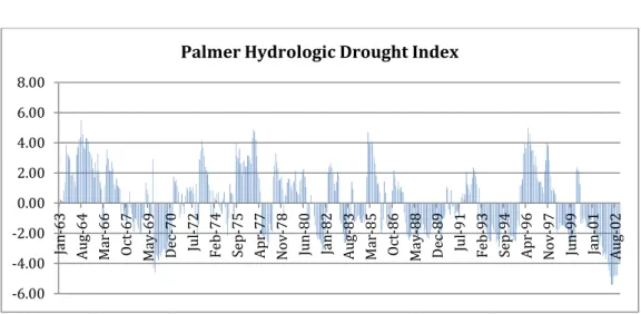
Palmer Drought Severity Index (PDSI) and Moisture Anomaly Index(Z)
The most prominent index of meteorological droughts is the Palmer Drought Severity Index (PDSI). The PDSI and the Z-index were both developed by Palmer (1965) and have been widely used in the scientific literature (Alley, 1984; Karl et
al., 1986). The PDSI was created with the intent of “measuring the cumulative
departure of moisture supply” (Palmer 1965).
The Palmer index is based on hydrological balance of soil and takes in account precipitation as well as evapotraspiration assuming as drought indicator the anomalies between the effective precipitation and the “climatically appropriated”.
In its original code arrangement, allows just analysis of historical droughts, thus a modified version, called PHDI (Palmer Hydrological Drought Index), has been applied by several public authorities in the USA to monitor drought condition, in order to implement a check and planning system in agriculture production.
The PDSI calculates a series of water balance terms for a generic two-layer soil model, and fluctuations in the hypothetical moisture supply, depending upon observed meteorological conditions, are compared to a reference set of water balance terms. This comparison leads to computation of the dimensionless PDSI.
Computation of the PDSI is complicated; for an in-depth discussion of the numerical steps, see Alley (1984). The PDSI is ideally a standardized measure of moisture conditions across regions and time. The shortcomings of regional comparability, which the PDSI was designed to facilitate, are further detailed by Guttman (1991). The PDSI is also imprecise in its treatment of all precipitation as rainfall, as snowfall may not be immediately available as water in the two-layer soil scheme.
The PDSI and Z-index are derived using a soil moisture/water balance algorithm that requires a time series of daily air temperature and precipitation data, and information on the available water content (AWC) of the soil. Soil moisture storage is handled by dividing the soil into two layers. The top layer has a field capacity of 25 mm, moisture is not transferred to the second layer until the top layer is saturated, and runoff does not occur until both soil layers are saturated. Applying the two-layer water budget model proposed by Palmer (1965):
AWC (mm) = AWCs + AWCu
where AWCs is referred to the superficial layer of the soil that can be assumed to be constant and equal to 25,4 mm while AWCu is referred to the underlying soil structure and depends on soil characteristics and thickness of root system.
Potential evapotranspiration (PE) is calculated using the Thornthwaite (1955) method condensed in the formula:
and water is extracted from the soil by evapotranspiration when PE > P (where P is the precipitation for the month). Evapotranspiration loss from the surface layer of the soil (Ls) always is assumed to take place at the potential rate. It is also assumed that the evapotranspiration loss from the underlying layer of the soil (Lu) depends on the initial moisture conditions in this layer, PE, and the combined available water content in both layers.
The Z-index is a measure of the monthly moisture anomaly and it reflects the departure of moisture conditions in a particular month from normal (or climatically appropriate) moisture conditions (Heim, 2002). The first step in calculating the monthly moisture status (Z-index) is to determine the expected evapotranspiration, runoff, soil moisture loss, and recharge rates based on at least a 30-year time series. A water balance equation is subsequently applied to derive the expected or normal precipitation. The monthly departure from normal moisture, d, is determined by comparing the expected precipitation to the actual precipitation. The Z-index, Zi, then is the product of d and a weighting factor K for the month i,
Zi=diKi
where Ki is a weighting factor that is initially determined using an empirically derived coefficient, K', and then adjusted by a regional correction factor that is used to account for the variation between locations. Monthly values of Ki are calculated using
where D is obtained during the calibration period by determining the mean of the absolute values of d for each month of the year.
The PDSI, indicated by Xi, is a combination of Zi, for the current month, and the PDSI value for the previous month,
While both the Z-index and the PDSI are derived using the same data, their monthly values are quite different. The Z-index is not affected by moisture conditions in the previous month, so Z-index values can vary dramatically from
month to month. On the other hand, the PDSI varies more slowly because antecedent conditions account for two-thirds of its value. Although the PDSI was designed to measure meteorological drought, it may be more appropriate as a measure of hydrological drought and, according to Karl (1986), the Z-index may be a better measure of meteorological or agricultural drought. It should be noted that although both the Z-index and PDSI are strongly weighted by both precipitation and temperature anomalies, most other meteorological indices (e.g., SPI, EDI, percent normal, deciles) are calculated using only precipitation. Alley (1984), Karl (1986), and Guttman (1998) have completed detailed evaluations of the limitations of the PDSI and Z-index, their work, along with the work of other researchers, has been summarized by Heim (2002). On the positive side, the PDSI does factor in antecedent conditions and is calculable from basic data. But its empirical nature, coupled with the fact it was developed for U.S. agricultural regions, limits its broad applicability, and as a result the PDSI is not used internationally. (Gibbs and Maher, 1967), Hayes (2000) considered its application for Australia but instead recommended rainfall deciles.
Cancelliere et al. (1996) verified the applicability of Palmer index in the Mediterranean area, selecting some basin located in Sicily, Greece and Cyprus. Comparison among PHDI and rolling mean values of some hydrologic variables, for different periods, shows a good correspondence of relative results.
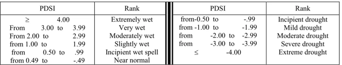
The PDSI is a dimensionless number typically ranging between 4 and 4, with negative quantities indicating a shortage of water as shown in table 2.II.
Table 2.II – Climatic classification according to Palmer Index
PDSI Rank PDSI Rank
4.00 From 3.00 to 3.99 From 2.00 to 2.99 from 1.00 to 1.99 from 0.50 to .99 from 0.49 to -.49 Extremely wet Very wet Moderately wet Slightly wet Incipient wet spell
Near normal from-0.50 to -.99 from -1.00 to -1.99 from -2.00 to -2.99 from -3.00 to -3.99 -4.00 Incipient drought Mild drought Moderate drought Severe drought Extreme drought
2.2.2 Hydrological drought indices
Hydrological droughts are associated with the impact of prolonged precipitation deficiencies on water supply from surface or subsurface sources such as rivers, reservoirs and groundwater (Keyantash and Dracup, 2002). Similarly, the American Meteorological Society defines hydrological drought as “Prolonged
period of below-normal precipitation, causing deficiencies in water supply, as measured by below-normal streamflow, lake and reservoir levels, groundwater
levels, and depleted soil moisture content”. The drought indices reviewed in this
section can be used to represent hydrological droughts.
There is an inherent time-lag between meteorological drought and hydrological drought because it takes longer for the precipitation deficiency to be reflected in streamflow and reservoir levels. This is especially important in places where groundwater is a major contributor to the streamflow and reservoirs. After a hydrological drought becomes established, even if the precipitation level returns to normal, it takes time for the hydrological drought to end. The time-lag will be small in areas with high precipitation and small reservoirs, because storm flows usually fill up the reservoirs to pre-drought levels. The time-lag will be large in areas of low precipitation and where spring discharge (from snowmelt) accounts for a significant amount of the total annual flow.
Drought indices such as Surface Water Supply Index (SWSI) (Shafer and Dezman, 1982) and Palmer Hydrological Drought Index (PHDI) (Karl, 1986) are commonly used to monitor hydrological drought. Further are also considered other indices like the Standardized Streamflow Index (SSI), Streamflow Deficit Index (SDI), Standardized Reservoir Index (SRI), and the Reservoir Deficit Index (RDI). These four indices are based directly on the reservoir and streamflow data, but these indices use a different standardizing procedure.
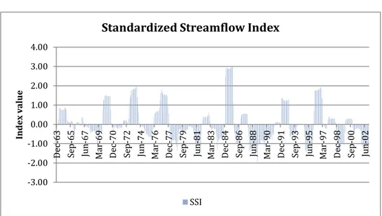
Standardized Stream-flow Index
The Standardized Streamflow Index (SSI), specifically developed for this study demonstrates great promise for monitoring hydrological drought. SSI is a standardized measure of streamflow that is similar in formulation to the SPI. McKee et al. (1993) developed a standardizing procedure for evaluating precipitation departures (e.g., SPI) using a probability distribution function. A similar approach was used to develop the Standardized Streamflow Index (SSI).
The computation on a monthly time step of SSI consists of following steps: Compute rolling cumulative monthly stream flow for several
aggregation time scales for the range of years based period of record; For each time scale, for each month of the year, fit a transformation to
convert the data into some probability function distribution: for the sake of consistency we assumed that the transformed data fit the normal distribution function;
Compute the mean and standard deviation of the transformed data; Compute the Z values in a standard normal distribution (i.e., Z = (X –
SSI is very similar to the standardized and deseasonalized stream-flow aggregated at correspondent time scale. The standard stream of 30-day mean flow would be equivalent to the SSI-k1 calculated using 30-day cumulative stream flow.
Surface water supply index (SWSI)
The Surface Water Supply Index (SWSI) is a hydrological drought index that was developed by Shafer and Dezman (1982) as an indicator of surface water conditions in order to replace the PDSI in areas where local precipitation is not the sole (or primary) source of streamflow (Shafer and Dezman, 1982). SWSI was designed for mountainous locations with significant snowfall because of the delayed contribution of snowmelt runoff to surface water supplies. The SWSI is calculated based on the monthly non-exceedance probability which is determined using available historical records of reservoir storage, streamflow, precipitation, and snowpack. Using a basin-calibrated SWSI algorithm, weights are assigned to each hydrological component based on its typical contribution to the water supply Then SWSI is calculated as a sum of the products of the probability of each the hydrological components and their respective weights.
It considers rainfall, streamflow/snow water content, and reservoir storage volume in formulating SWSI.
The mathematical formulation of the SWSI is as follows:
where, PN is the probability of non-exceedance (%); rn, sf, sn, and rs is refer to rainfall, streamflow, snow water content and reservoir storage volume components respectively; a, b, c are weights for each component and must meet the condition a+b+c = 1. Subtracting 50 and dividing by 12 are a centering and compressing procedure designed to make the index value have a similar magnitude to the PDSI (Palmer, 1965).
Because it is dependent on the season, the SWSI is calculated using only reservoir storage, snowpack, and precipitation during the winter (December through May). During the rest of the year (June to November) streamflow replaces snowpack in the SWSI equation. Calculations are performed on a monthly time step. Monthly data are collected and summed for all locations where reservoir storage, streamflow, precipitation, and snowpack are measured in the basin.
Each component is normalized using the historical data. The probability of non-exceedance (e.g., the probability that subsequent values of that component will
not exceed the current value) is determined for each component using frequency analysis. Converting all of the components to a non-exceedance probability allows their values to be compared to each other. The SWSI, similar to PDSI, has an arbitrary scale that is centered on zero and ranges from –4 to +4 as follows (Shafer and Dezman, 1982): 4.0+, abundant supply; 2.0+, Near normal; -1.0, incipient drought; -2.0, moderate drought; -3.0, severe drought; and -4.0, extremely drought.
SWSI is a particularly good measure of surface water supply conditions because it accounts for the major hydrological variables that contribute to surface water supply there.
2.2.3 Agricultural drought indices
Crop moisture index
Palmer (1968) developed the Crop Moisture Index (CMI) to monitor short-term changes in moisture conditions affecting crops. The CMI is the sum of an evapotranspiration deficit (with respect to normal conditions) and soil water recharge. These terms are computed on a weekly basis using PDSI parameters, which consider the mean temperature, total precipitation, and soil moisture conditions from the previous week (Palmer 1968).
The CMI can assess present conditions for crops, but it can rapidly vacillate and is a poor tool for monitoring long-term drought (Hayes 2000). For example, a rainstorm may briefly bring crops adequate moisture, even though an extended drought persists. The CMI also begins and ends each growing season near zero, which may be appropriate for botanical annuals, but not for tracking long-term drought. As a consequence, the assessment of agricultural drought is better suited to the related Palmer Z index (Karl 1986).
2.2.4 Operational indices
Multivariate Aggregate Drought Index
The Aggregated Drought Index (ADI) is a multivariate index developed by Keyantash and Dracup (2004) which derives a single value using Principle Component Analysis (PCA) over data from hydrological, meteorological, and agricultural drought regimes. The ADI is designed for use over regions of climatic uniformity, such as climate divisions defined by the Nation Climatic Data Center (NCDC) (Keyantash and Dracup, 2004). Its input variables represent the fluctuations in water volume within the hydrologic cycle; ADI incorporates several variables that define the hydrologic cycle and any combination of six parameters describing bulk water content within a climate division: Precipitation (P),
Evapotranspiration (E), Streamflow (Q), Reservoir Storage (V), Soil Moisture Content (W), and Snow Water Content (s). The ADI is flexible such that the entire suite of parameters or just selected variables can be used over each time step, since each time step is treated independently. Keyantash and Dracup, 2004 were able to correlate the ADI with severe droughts in three California climate divisions.
The Principal Component Analysis (PCA) was used to aggregate the aforementioned variables. Computation of the Principal Components (PCs) requires constructing a square (p x p, where p is the number of variables) symmetric correlation matrix to describe the correlations between the original data. The PCs are a re-expression of the original p-variable data set in terms of uncorrelated components Zj (1 < j ≤ p). Eigenvectors derived through PCA are unit vectors (i.e., magnitude of 1) that establish the relationship between the PCs and the original data:
Z = XE
where, Z is the n x p matrix of PCs (i.e. uncorrelated components); in which n is the number of observations, X is the n x p matrix of standardized observational data, and E is the p x p matrix of eigenvectors.
As was done by Keyantash and Dracup (2004), the ADI was considered as the first PC (PC1), normalized by its standard deviation:
where, ADIi,k is the ADI value for month k in year i, Zi,k is the first PC during year i for month k, and σ is the sample standard deviation of Zi,k overall years for month k.
The ADI utilizes only the PC1 because it explains the largest fraction of the variance described by the full p-member standardized data set.
2.3 Calculation of indices and drought classification
Drought events are selected from the indices time series using the threshold level method (e.g. Yevjevich, 1967), which defines the drought as a period when the variable analyzed is below a certain threshold value (i.e. in a deficit situation). At each time step the start and end of the drought is identified. The following characteristics are derived for each event:
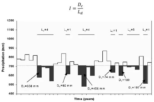
drought duration average deficit volume drought magnitude
As defined by Yevjevich (1967), the duration Ld of a drought event j is assumed as the number of uninterrupted time steps (in the present study: months) with a state variable below the threshold for one or more time steps:
The average deficit volume of a drought event j over the catchment area is defined as the sum of the deficit volumes over an uninterrupted number of months with the state variable below the classification threshold for one or more time steps:
where Dc is the deficit volume.
While the drought magnitude is given by the ratio between cumulative deficit and duration:
Figure 2.2 – Identification of duration and deficit of an hydrologic variable with the threshold level methods (Yevjevich, 1967)
To detect drought events, adopted thresholds were the numerical limits of drought classification proposed by respective authors of indices (reminded above) and applied to correspondent time series. An indicator function is introduced, which specifies that a drought occurs, if true (=1, below the threshold) and a non-drought condition occurs, if false (=0, above the threshold).
2.4 Criticism of existent drought indices
The first step in determining which meteorological and hydrological drought indices are the most appropriate for monitoring drought conditions at the local level was to review the scientific literature and compile a list of the strengths and weaknesses of each index. In this section the data requirements of each drought index will also be described since the purpose of this study is to identify drought indices that can be calculated operationally. Therefore the “best” drought indices are those that can be calculated using readily available data. Only those indices that are critiqued in the literature have been included in this section.
The PDSI, PHDI, and Z-index are all calculated using the algorithm that was developed by Palmer (1965) and therefore, for simplicity, all of the discussion will use the term PDSI to refer to all three of these indices.
The PDSI is calculated using temperature and precipitation data. The daily temperature and precipitation data are aggregated to weeks or months, depending on the time-scale of interest. The PDSI also needs information on the available water holding capacity of the soil. Since the PDSI uses the Thornthwaite (1948) method for estimating PET, the latitude of the location also needs to be provided.
The PDSI was the first comprehensive drought index developed in the U.S. and it is widely used for drought monitoring and within state drought plans (Heim, 2002). Despite its widespread use, the PDSI has many limitations. One of the limitations of the PDSI is that PET is estimated using Thornthwaite’s method (which only considers monthly temperatures to estimate PET) (Narasimhan and Srinivasan, 2005). More realistic estimates of PET can be generated by using a physically-based method such as the FAO Penman-Montieth equation (Allen et al., 1998). However a recent study determined that calculating the PDSI with a more physically-based method of calculating ET did not improve the correlation between the PDSI and soil moisture at the study sites (in Greece).
Another limitation of the PDSI is that it uses a two layer soil model with just a single parameter for the available water holding capacity of the soil. This may be reasonable when calculating the PDSI for a single location (e.g., station), but it is inappropriate for calculating the PDSI for regions, such as climate divisions within which the soil is highly spatially heterogeneous (Narasimhan and Srinivasan, 2005). There is no way to represent the horizontal and vertical heterogeneity of soil
properties in the PDSI water balance. It is important to use an appropriate value for the available water holding capacity of the soil because it has been demonstrated that the PDSI is sensitive to changes in this parameter (Karl, 1986).
The PDSI also assumes that runoff only occurs when the two soil layers are both completely saturated. In reality runoff varies due to differences in slope, soil type, land use, land cover, and land management practices (Narasimhan and Srinivasan, 2005). None of these factors are accounted for in the PDSI. Alley (1984) noted that there are also problems with how runoff is generated because the model does not account for the distribution (or intensity) of precipitation within the week or month. The PDSI also does not account for the seasonal changes in vegetation growth and root development and it is not designed to deal with a snowpack or frozen soil (Alley, 1984; Karl, 1986; Karl et al., 1987).
PDSI is highly dependent on the weighting factor used to make it comparable between different regions (and months) (Heim, 2002). Palmer (1965) calculated the regional correction factor (K) based on data from only nine locations in seven states and calculated the duration factors 0.897 and 1/3 based on data from western Kansas and central Iowa and they affect the sensitivity of the index to precipitation events (Wells et al., 2004). An improvement proposed by Wells et al. (2004) is meant to correct the lack of spatial comparability by dynamically calculating the regional correction factor (K) and the duration factors using historical climate data from each location.
The original formulation of the PDSI is known to be spatially and temporally variants and therefore it cannot be compared across different countries or between months (Alley, 1984; Guttman et al., 1992; Guttman, 1998; Heim, 2002). This means that severe and extreme droughts as defined by the PDSI occur more often in some parts of the country than others (Wells et al., 2004).
The length of the calibration period (historical record) will have an influence on the stability of the estimated parameters. Longer calibration periods tend to provide more consistent PDSI values (Karl, 1986). For comparison purposes, the same calibration period should be used for all locations. Interpreting the PDSI can also be a challenge since it is a function of both temperature and precipitation data. It has been demonstrated that the PDSI responds in a non-linear fashion to changes in precipitation.
Although the PDSI is often defined as a meteorological drought index the PDSI responds rather slowly to changes in moisture conditions. According to Guttman (1998), the PDSI has a ‘memory’ (its spectrum conforms to that of an autoregressive process) and it is highly correlated with the 12-month SPI (Heim, 2002). This means that both the PDSI and PHDI are more appropriate for measuring hydrological droughts. The Z-index can be used for measuring
agricultural and meteorological drought since it only accounts for the moisture conditions during the current week or month.
The drought classification that was proposed by Palmer (1965) was arbitrarily determined, so those thresholds are not appropriate for making water management decisions or triggering drought response programs or declarations of drought emergency unless they have been confirmed by an independent local assessment (Alley, 1984). It has also been demonstrated that the calculation procedure for transitioning between wet and dry spells tends to produce an asymmetrical and bimodal distribution of PDSI values (Alley, 1984; Heim, 2002). Therefore, the PDSI is not normally distributed and cannot be interpreted in the same way as other indices, such as the SPI.
Speaking on which, SPI is a popular drought index because of its simplicity and versatility. To calculate the SPI one only needs weekly or monthly precipitation data (depending on the time scale on the intended application). The SPI can be calculated for any time period of interest.
Time-scales are appropriate for monitoring different types of drought and correspond to different drought impacts. Unlike the PDSI, the SPI is spatially invariant (Guttman, 1998; Heim, 2002; Wu et al., 2007) and so values of the SPI can readily be compared across time and space. Although the SPI can be calculated in all climatic regions (Heim, 2002), it is important to note that arid regions, those that experience many months with zero precipitation, may be problematic for the SPI depending on which PDF is used to normalize precipitation (Wu et al., 2005). The SPI is also easier to understand and interpret than the PDSI since its value is only based on precipitation and since it is reported in standard deviations away from the mean.
However, there are some limitations associated with the SPI. Like the PDSI, it is computationally complex (it cannot be calculated by hand or with a spreadsheet) and it requires specialized code. The SPI also requires a long (and complete) precipitation record.
It has been demonstrated that the SPI is strongly influenced by record length (Wu et al., 2005). Therefore when comparing stations to each other, it is best if they have the same length of precipitation record. The minimum precipitation record for calculating the SPI is 30 years, but it is recommended to use 50+ years of data (and the extreme values of the SPI may only be accurate when even longer precipitation records are used (80+ years)) (Wu et al., 2005).
It can also be demonstrated that the SPI will be strongly influenced by the presence of missing data (and the interpolation/replacement of missing data). This analysis demonstrates that decisions that are made about how missing data is handled will have a direct impact on the magnitude of precipitation-based drought indices such as the SPI.
The SPI is also influenced by normalization procedure (e.g., PDF selection) that is used. Guttman (1999) analyzed six different PDFs (including: the two-parameter gamma; the two-two-parameter gamma, for which the two-parameters are estimated by the maximum likelihood method; the three-parameter Pearson Type III; the three-parameter generalized extreme value; the four-parameter kappa; and the five-parameter Wakeby) and determined that the Pearson Type III was the most appropriate PDF for calculating SPI. Using a different PDF will generate different SPI values.
Vicente-Serrano and Begueria (2003) point out that drought indices are not as useful in identifying spatial patterns of drought risk since they are based on standardized or normalized shortages in relation to “average conditions”, which relate to a given station and a given period. This holds true for both the SPI and the PDSI indices. As a result, the frequency of drought spells is about the same for all stations no matter if they lie in extremely arid or extremely rainy regions, even though the rainy sites may receive several times more rain than the arid sites. Similarly, these indices cannot be used in climate-change impact assessments, as they would provide approximately the same distributions for both present and changed climates regardless of the changes in the climatic conditions.
Regarding the Standardized Streamflow Index, one of the main advantages is that it can be calculated for a wide range of time scales and, using daily data, it can be updated on a daily rather than monthly basis. Therefore it can be used to monitor short, medium, or long-term hydrological drought in near-real time. The index is a standardized measure of streamflow based on a statistical measure and so it is more robust that just using streamflow departures. Interpretation of SSI is straightforward, negative values indicate below normal streamflow and positive values indicate above normal streamflow. Since the index is standardized, it can be compared across space and time.
One of the main weaknesses of the SSI is that it is very difficult to fit a statistical distribution to the raw cumulative streamflow data (Serrano et al. 2012), hence the data has to be transformed and. even after being transformed, especially during low-flow periods and for short-accumulation time scales, the data did not fit a normal distribution. This could potentially introduce errors in the calculation of the index. Also it is difficult to find gage records that are appropriate for calculating the SSI since there are a limited number of long streamflow records for gages unaffected by upstream reservoirs.
2.5 About areal extent of drought
Although the estimation of drought severity and duration at watershed scale gives useful information for water management, it is interesting and important to assess drought over a wider region by considering also the areal extension of the drought.
The regional analysis consents to determinate general characteristics and spatial distribution of droughts, as well as an evaluation of the most affected areas where socio-economic and environmental impacts are relevant: a more exhaustive awareness of these natural extreme events is indispensable for adequate planning and implementation of effective mitigation measures.
To reach this purpose Yevjevich, in 1967 proposed the method of run to detect at-site droughts; effectively it can be extended in the analysis of regional droughts by considering time series of the variable used as parameter of the study and for which are available measurements registered at several stations and selecting, besides the truncation level at each site, an additional threshold, which represents the value of the area affected by deficit above which a regional drought is considered to occur (Santos, 1983).
The statistical properties of such detected droughts can be then investigated; for example Rossi (1983) analyzed the historical series of areal coverage and regional deficit in order to verify whether the two characteristics differ significantly over different basin to assess the possibility of adopting an interbasin water transfer as a drought mitigation measure.
Alternatively, characteristics of drought indices could be investigated by means of statistical tools in order to obtain the probability distribution function of the indices. Further, the Monte Carlo method can be applied simulating the characteristics of drought indices over a large region, as in the study of Tase (1976) and Tase and Yevjevich (1978).
Several methods can be adopted to describe historical regional drought events requires, through the investigation of the spatial variability of the underlying variable or, as an alternative, of a drought index. One of the commonly adopted method for analyzing spatial variability of drought events is by drawing isoline maps of a drought descriptor, such as:
the rainfall depth at the time interval i, expressed as a percentage of the corresponding long term mean;
the deviation of the total rainfall computed on a past drought period from the corresponding long term mean, namely the rainfall deficit, expressed as absolute value or ratio or percentage of the mean;
the standardized deficit obtained as the ratio, for a given time interval, of the rainfall deviation from the mean over the standard deviation. Also, the areal extent of an historical drought can be drawn by plotting a drought descriptor versus the corresponding percentage areal coverage.
Alternatively, the relationship between a drought descriptor of selected probability of occurrence and the corresponding percentage areal coverage can be adopted to analyze spatial variability of droughts. Among the latter category, drought severity-area-frequency (SAF) curves have been proposed for assessing drought in a region.
One of the first works on SAF curves has been carried out by Rossi (1983). In this study, curves relating the areal weighted (by means of Thiessen polygons) precipitation deficits of fixed return period to the corresponding areal coverage are derived with reference to different aggregation time periods for Sicily region, Italy. The approach generally adopted to derive SAF curves consists of the following steps (Kim et al., 2002; Loukas and Vasiliades, 2004;Mishra and Desai, 2005;Mishra and Singh, 2008):
identify the variable at a suitable time scale (e.g. monthly precipitation) to be used for estimating drought characteristics;
spatially interpolate local values on a fixed point grid;
identify drought and drought characteristics (e.g. by applying the theory of runs or by computing one or more drought indices for each gridded time series);
estimate a measure of drought severity (e.g. sum of negative runs in a dry spell, sum of negative SPI values in a dry spell, etc.) associated with different areal extents (in terms of percentage area) by considering different areal threshold;
determine the best probability distribution fitting drought severity series for different areal extents;
perform frequency analysis in order to associate drought severity with different return periods;
CHAPTER 3
3 M
ETHODOLOGIES OFD
ROUGHTA
NALYSIS ATD
IFFERENTS
PATIALS
CALES3.1 Introduction
In previous chapter some of the most common indices generally adopted to characterize and monitor drought events have been presented, also with reference to the required data and calculation procedures.
In this part of the thesis methodologies presented in the research are discussed. Substantially the chapter is addressed in three main arguments:
In the first part are presented methodologies to compare results coming from drought analysis carried out implementing most common drought indices;
In the second part a method of aggregation of those drought indices into a unique indicator is illustrated;
In the third part a methodology to explore the severity of drought areal extent and to characterize probabilistically his frequency is discussed. In order to achieve the objectives of the research three of the presented indices have been selected to carry on the drought analysis: the Standardized Precipitation Index, the Standardized Streamflow Index and the Palmer Hydrologic Drought Index. Furthermore, they have been functional to the local drought analysis, while the SPI has been selected as drought variable to achieve the probabilistic regional investigation.