Circularly polarized antennas

(1)

UNIVERSIT `A DEGLI STUDI DI CATANIA

Dipartimento di Ingegneria Elettrica Elettronica ed Informatica

Dottorato di Ricerca in Ingegneria Informatica e delle Telecomunicazioni

XXVI Ciclo

CIRCULARLY POLARIZED ANTENNAS

Ing. Ornella Leonardi

Coordinatore

Chiar.ma Prof. V. Carchiolo

Tutor

(2)

(3)

Acknowledgment

I wish to thank my tutor Prof. Eng. Gino Sorbello for his unwavering support and encouragement over the last three years, for his generous mentorship and friendship. I consider it a privilege to have been his student. I have learned a tremendous amount from him, and his personal and professional example has meant a great deal to me.

I wish to thank Eng. Tindaro Cadili from Selex-ELSAG, site of Catania, for the use of the anechoic chamber facility to performed the experimen-tal characterization of cross-slot coupled antenna.

I wish to thank Eng. Mario Pavone from StMicroelectronics for the experimental realization of elliptical-slot patch antenna.

I wish to thank Eng. Antonio Levanto from Technical Support Team ANSYS Electromagnetic for the countless loose knots in the use of HFSS simulator.

Also i wish to thank two great colleagues and friends, P. Di Mariano and L. Nicolosi, for their contribution to the experimental measurements and for their unwavering support and encouragement over the last year. Most of all, I would like to thank my husband, Antonio, and my parents whose love, support and patience make this possible.

(4)

(5)

Abstract

In recent years low profile, lightness, compactness, easy manufacturing and integrability with solid-state devices on a circuit board have become a priority in the antenna design. Microstrip antennas are a possible answer to these new requirements in several areas, such as remote sensing, mobile satellite and cellular communications, direct broadcast satellite (DBS) system and global positioning system (GPS).

Many of the above mentioned applications make use of circularly pola-rized antennas. However, such requirement in planar microstrip antenna is not a trivial task since many factors have to be considered including fabrication tolerance and systematic errors in the manufacturing process. In the present thesis we address the task to achieve circular polariza-tion with very compact planar antennas in two ways:

1) a more conventional one dealing with two innovative designs;

2) a less conventional one through of artificial materials, such as High Impedance Surface (HIS).

As far as the first point is concerned, two standard designs have been developed for a Dedicated Short Range Communication (DSRC) system. In particular, we have proposed two innovative compact antennas that represent a step forward with respect to other available DSRC solution.

(8)

The two proposed antenna prototypes have been optimized, fabricated and experimentally tested. They represent an answer to the need of achieving good circularly polarized antennas in a small mobile On-Board Unit (OBU) of a DSRC system.

As a further study, we have considered to improve performance such as the radiated power, the gain and the directivity, or to reduce the global antenna thickness. For this reason we have developed a full-wave model for periodic surface and considered their employment to achieve circular polarization. As a proof of concept, we have tested a simple arrangement that allows circular polarization of the radiated field.

The thesis is organized as follows.

In the first part, we briefly introduce some relevant technical features of microstrip antenna’s. Then the properties of circular polarized waves are discussed, with particular interest in wireless communications. The circular polarization quality factors and antenna measurement setup are briefly introduced and discussed.

In the second part, we address the design and the experimental cha-racterization of two circularly polarized microstrip patch antenna proto-types.

In the last part of the thesis, High Impedance Surfaces (HIS) are briefly introduced. Then, a simple FEM-model is presented and com-pared with the standard FTDT-model used in literature. In this respect, a rectangular-array-patch working as HIS surface is considered and tested to achieve circular polarization with a printed dipole.

(9)

Chapter 1 Microstrip Antennas

In this chapter we discuss some of the microstrip antenna’s technical fea-tures. We consider their advantages and disadvantages, including sub-strate material consideration, excitation techniques, polarization behav-iors, bandwidth characteristics, and miniaturization techniques. The mi-crostrip antenna radiation properties and analysis techniques are briefly presented.

1.1 Advantages and limitations

The microstrip antennas are nowday widely used in telecommunications systems, in fact they are employed in applications with working frequen-cies ranging from 100 MHz to 100 GHz, such as radar systems, satellite communications, mobile communications and wireless LAN. Their suc-cess is due to the many advantages of microstrip antennas compared to conventional counterparts. Among the advantage we list:

• relatively low production cost

(10)

• reduced volume and weight

• simpler integration with other electronic devices

• possibility to achieve linear and circular polarization with single feeding.

The major disadvantages of microstrip antennas are:

• higher ohmic and dielectric losses as compared to conventional so-lution

• low efficiency

• low directivity (6-8 dB) • reduced gain (about 6 dB)

• high quality factor Q, which results in a very narrow bandwidth • spurious radiation due to feed

• poor polarization purity

• complex electromagnetic analysis of the structure.

However, there are several methods to increase the radiation efficiency and the bandwidth, such as using structures with multiple substrate layers with different heights and dielectric constant. However complex multiple layer structure may support unwanted superficial waves that can be suppressed with the aid of special periodic structures known as AMC surface (see chapter 4).

(11)

1.2. Feeding Methods 5 Microstrip antennas consist of a very thin metallic patch (17 < hmetal < 35 µm) separate from a ground plane by a

dielec-tric substrate, with thickness d << λ and with relative dielecdielec-tric constants between in the range of [2.2 ÷ 12]. The metallic patches are the radiating elements and are usually photoetched on the dielectric substrate, these may be rectangular, circular, square, elliptical or any forms. The patch is connected to a RF source o to a receiver through a feeding line which can be a microstrip line. The main feeding techniques are discussed briefly in the next section.

Lower dielectric constant and thick substrate are desirable for anten-nas requiring high efficiency and larger bandwidth, whereas thin sub-strate and higher dielectric constants are required for feeding network where it is necessary to keep the fields well confined to avoid unwanted radiation and coupling losses. These requirements make it almost im-possible to produce a good antenna on a single substrate. However, by separating the feed network from the radiating element, and providing aperture coupling between them it is possible to meet both the above requirements.

1.2 Feeding Methods

The feeding technique allow the control of the input impedance as well as the radiation characteristics of the antenna. The choice and optimization of feeding network is an important task in microstrip antenna design. The miscrostrip antenna can be excited directly either by a coaxial probe or by a microstrip line, otherwise indirectly using electromagnetic coupling through aperture coupling or by coplanar waveguide feed, in which case

(12)

there is no direct metallic contact between the feed line and the patch. The coaxial or probe feed arrangement requires that the center con-ductor of the coaxial connector is soldered to the patch. The main ad-vantage of this feed is that the feeding point can be placed at any desired location inside the patch to match a desired impedance. The disadvan-tages are that the hole has to be drilled in the substrate and that the connectors protrudes outside the bottom ground plane, so that it isn’t planar to the structure. Also this feeding arrangement makes the config-uration asymmetrical.

The microstrip line feed arrangement (see figure 1.1 a) has the advan-tage that it can be etched on the same substrate, so the total structure remains planar. The drawback is the radiation from the feed line, which leads to an increase in the cross-polar level. Also, in the millimeter-wave range, the size of the feed line is comparable to the patch size, leading to increased undesired radiation.

In the electromagnetic coupling feed arrangement (see figure 1.1 b), also known as proximity coupling, a two dielectric layer structure is used and the feed line is placed between the patch and the ground plane. The advantages of this feed configuration include the reduction of spurious feed-network radiation. The disadvantages are that the two layers need to be aligned properly and that the overall thickness of the antenna increases.

In the aperture-coupled arrangement (see figure 1.1 c), the field is coupled from the microstrip line feed to the radiating patch through an electrically small aperture or slot cut in the ground plane. The cou-pling aperture is usually centered under the patch, leading to lower cross-polarization due to symmetry of the configuration. The slot aperture can be either resonant or not; in the first case provides another resonance in

(13)

1.3. Antenna parameters and fundamental limitations 7

Figure 1.1: Feeding arrangements. (a) microstrip line, (b) electromagnetic coupling,(c) aperture coupling, and (d) coplanar waveguide (CPW).

addition to the patch resonance thereby increasing the bandwidth at the expense of an increase in back radiation.

In the coplanar waveguide arrangement (see figure 1.1 d) the CPW is etched on the ground plane of the microstrip. The coplanar waveguide is terminated by a slot. The main disadvantage of this method is the high radiation from the rather longer slot, leading to the poor front-to-back ratio. The front-to-front-to-back ratio can be improved by reducing the slot dimension and/or by modifying its shape, for example to form of a loop.

1.3 Antenna parameters and fundamental

limitations

From the circuit point of view, an antenna is a single port device. An input signal in the form of an incident wave traveling along the transmis-sion line flows from the signal source toward the antenna. Assuming the

(14)

amplitude of the incident wave is V+ _{at the antenna port, some of the}

energy carried by the incident wave is radiated by the antenna. In the meantime, the residual energy is reflected at the port and travels back along the transmission line. The amplitude of the reflected wave is V−. The voltage reflection coefficient is given by:

Γ = V− V+

When designing an antenna, the goal is to minimize the reflection at the antenna port, as low as possible ideally ( Γ ≃ 0 ), that is make sure that a perfectly matched antenna is achieved.

In microwave theory, the S-parameter matrix is used to quantitatively describe a multi-port network. For an antenna its S-matrix degenerates to a single element, S11, it is defined by the ratio of the voltages of

incident and reflected wave, then:

S11 = Γ

In engineering the S11 is often defined as the ratio of incident and

re-flected power:

S11(dB) = 20 log10(|S11|)

The absolute value of S11 (dB) is called the Return Loss (RL):

RL = −S11(dB)

The other commonly used parameter is Voltage Standing Wave Ratio (VSWR), it is the ratio of the amplitude of a partial standing wave at an antinode (maximum voltage) to the amplitude at an adjacent node (minimum voltage), in an electrical transmission line:

V SW R = |Vmax| |Vmin|

(15)

1.3. Antenna parameters and fundamental limitations 9 Bandwidth is another important parameter used to describe antennas, it is defined as the frequency range over which a particular requirement is fulfilled. For example the impedance bandwidth is the frequency range over which VSWR is less than 2, which corresponds to a return loss of 9.5 dB or 11% reflected power. We defined the fractional bandwidth as the normalized spread between the half-power frequencies :

BW = fmax− fmin foperative

= 1 Q where Q is the Quality Factor.

The quality factor is representative of the antenna losses:[1]

1 Q = 1 Qrad + 1 Qc + 1 Qd + 1 Qsw

where Qrad is the contribution due to radiation losses, Qc is the

contri-bution due to conduction (ohmic) losses, Qd is the contribution due to

dielectric losses and Qsw is the contribution due to surface waves.

For very thin substrate the losses due to surface waves are very small and can be neglected, while the Qrad is inversely proportional to the height

of the substrate and then it is usually the dominant factor.

The parameter which tells us how well an antenna can radiate is the Efficiency, it is the ratio of the power radiated by the antenna to the power delivered to the input terminals of the antenna, it is commonly expressed in dB :

Efficiency (dB) = 10 log₁₀ Pradiated Pavailable

It can also be expressed in terms of the quality factors: Efficiency =

1 Qrad

1 Qc

(16)

The quality factor, bandwidth and efficiency are then antenna figures of merit which are correlated and there isn’t complete freedom to indepen-dently optimize each one. Therefore there is always a trade-off between them to arriving at an optimum antenna performance.

1.4 Analysis Techniques: an overview

With an analysis technique, the engineer should be able to predict the antenna performance qualities, such as the input impedance, resonant frequency, bandwidth, radiation patterns, and efficiency. There are many different techniques of analysis for design microstrip antennas that can be divided into two broad categories:

• analytical solution of an idealized model approximation • numerical method

In the first group make use of equivalence theorem and magnetic equi-valent sources to model the patch edges, the most used are:

• Transmission-line Circuit Model[2]

• Cavity Model[3]

• Multiport Network Model, MNM[4]

[2]_{Munson, “Conformal microstrip antennas and microstrip phased arrays”.} [3]_{Richards, Lo, and Harrison, “An improved theory for microstrip antennas and}

applications”.

[4]_{Gupta and Sharma, “Segmentation and Desegmentation Techniques for the}

(17)

1.4. Analysis Techniques: an overview 11 Numerical method are based on the numerical solution of the distribu-tions of real electric currents on the patch and the ground plane, between which the most important are:

• Method of Moment, MoM[5]

• Finite-Difference Time Domain, FTDT[6]

• Finite-Element Method, FEM[7]

1.4.1 Approximate Models

In the Transmission Line Model the microstrip radiator element is viewed as a transmission line resonator with no transverse field variations, the field only varies along the length, and the radiation occurs mainly from the fringing fields at the open circuited ends. The patch is represented by two slots that are spaced by the length of the resonator. Although the Transmission Line Circuit Model is simpler than the cavity model, it gives good physical insight, but is less accurate and more difficult to model coupling.

The Cavity Model is more accurate but more complex. In the cavity model, the region between the patch and the ground plane is treated as a cavity that is surrounded by magnetic walls around the periphery and by electric walls from the top and bottom sides. Since thin substrates are used, the field inside the cavity is uniform along the thickness of the

[5]_{Newman and Tulyathan, “Analysis of microstrip antennas using moment}

meth-ods”.

[6]_{Sheen et al., “Application of the three-dimensional finite-difference time-domain}

method to the analysis of planar microstrip circuits”.

(18)

substrate. The fields underneath the patch for regular shapes can be expressed as a sum of the various resonant modes of a planar resonator. The effect of the fringing fields can be taken into account by extending the patch boundary outward, so that the effective dimensions are larger than the physical dimensions of the patch. The effect of the radiation from the antenna and the conductor loss are considered by adding these losses to the loss tangent of the dielectric substrate. The far field and radiated power are evaluated, using the equivalence theorem, from the equivalent magnetic current around the periphery (see 1.4.3).

The Multiport Network Model is an extension of the cavity model. In this method, the electromagnetic fields underneath the patch and out-side the patch are modeled separately. The patch is analyzed as a two-dimensional planar network, with a multiple number of ports located around the periphery. The multiport impedance matrix of the patch is obtained from its two-dimensional Green’s function. The fringing fields along the periphery and the radiated fields are incorporated by adding an equivalent edge admittance network. The segmentation method is then used to find the overall impedance matrix. The radiated fields are obtained from the voltage distribution around the periphery.

1.4.2 Numerical Models

The Numerical Methods, also known as Full-Wave Model, are very accu-rate, very versatile, but they are the most complex and the more expen-sive from a computational point of view.

In the MoM, the surface currents are used to model the microstrip patch, and volume polarization currents in the dielectric slab are used to model the fields in the dielectric slab. An integral equation is

(19)

formu-1.4. Analysis Techniques: an overview 13 lated for the unknown currents on the microstrip patches and the feed lines and their images in the ground plane. The integral equations are transformed into algebraic equations that can be easily solved using a computer. This method takes into account the fringing fields outside the physical boundary of the two-dimensional patch, thus providing a more exact solution.

The FEM, unlike the MoM, is suitable for volumetric configurations. In this method, the region of interest is divided into any number of finite surfaces or volume elements depending upon the planar or volumetric structures to be analyzed. These discretized units, generally referred to as finite elements, can be any well-defined geometrical shapes such as triangular elements for planar configurations and tetrahedral and pris-matic elements for three-dimensional configurations, which are suitable even for curved geometry.

In the FDTD Method spatial as well as time grid for the electric and magnetic fields are generated. The solution is evaluated over such grids. The E cell edges are aligned with the boundary of the configuration and H-fields are assumed to be located at the center of each E cell. Each cell contains information about material characteristics. The cells containing the sources are excited with a suitable excitation, which propagates along the structure. The discretized time variations of the fields are determined at desired locations. Using a line integral of the electric field, the voltage across the two locations can be obtained. The current is computed by a loop integral of the magnetic field surrounding the conductor, where the Fourier transform yields a frequency response.

(20)

1.4.3 Cavity Model

Consider a simple microstrip patch antenna of any shape. Since the sub-strate has a thickness much smaller than both the wavelength and the size of the metal tracks, in first approximation, the electromagnetic field can be considered constant along the normal to the substrate. Initially we neglect the edge effect and we assume that the electric field has only a perpendicular component at the periphery of the substrate. This equals to ideally close transversely the perimeter of patch with Perfect Magnetic Conductor (PMC). In this way, the portion under the patch, for a rect-angular patch, can be studied as a resonant cavity closed by four PMC walls and two PEC walls.

We assume that the EM field is independent of thez coordinate or-_ thogonal to the substrate, the electric field has only the component Ez

while the magnetic field has transverse component, ⃗Ht, with respect to



z. By writing the solution of Maxwell’s equations for TM fields as a function of a magnetic vectorial potential A(x, y) = Az(x, y)ˆz and since

kz = 0, we have: Ez(x, y) = k2 jωϵAz(x, y) = −jωµAz(x, y) (1.1) Ht(x, y) = ∇tAz(x, y) × ˆz = 1 jωµˆz × ∇tEz(x, y) (1.2) Then the electric field satisfy the two-dimensional Helmholtz’s equa-tion:

∇2_tEz(x, y) + k2Ez(x, y) = 0 (1.3)

with the boundary condition ∂Ez

∂n = 0 where ˆn is the unit vector

(21)

1.4. Analysis Techniques: an overview 15 In Cartesian coordinates the equation (1.3) can be solved by the separation of variables method, then

Ez(x, y) = X(x)Y (y) (1.4)

X(x) = C1sin(kxx) + C2cos(kxx) (1.5)

Y (y) = D1sin(kyy) + D2cos(kyy) (1.6)

where k2 _{= k}2 x+ ky2.

Imposing the boundary condition ∂Ez

∂n = 0 over the perimeter of patch

and using the (1.2) we get: Ez(x, y) = C cos mπ L x  sinnπ Wy  (1.7) Hx = − 1 jωµ ∂Ez ∂y = C jωµ nπ W cos mπ L x  sinnπ Wy  (1.8) Hy = 1 jωµ ∂Ez ∂x = − C jωµ mπ L sin mπ L x  cosnπ Wy  (1.9) k2 = mπ L 2 +nπ W 2 m, n = 0, 1, 2... (1.10) Because k2 _{= ω}2_{ϵµ the resonance frequency are achieved by:}

fm,n = c 2π√ϵr  mπ L 2 +nπ W 2 m, n = 0, 1, 2... (1.11) The cavity field for the fundamental mode TM10 will be:

Ez(x) = C cos π Lx  (1.12) Hy(x) = − D jωµ sin π Lx  (1.13) and the resonance frequency will be:

f1,0 = 1 2 c0 L√ϵrµr (1.14)

(22)

(a) (b)

Figure 1.2: Rectangular microstrip patch antenna: (a) new reference system; (b) Cavity Model. The Electric Field ⃗E = Ez(x)uz is represented only around the perimeter at height h₂.

If we change reference frame equation (1.12)-(1.13) become:      Ez(x) = −E0sin _π Lx  Hy(x) = −H0cos _π Lx  (1.15)

To take account of the effects of the fringing fields we can consider an effective length in (1.14), where Leq = L + 2a. The corrective term 2a

is an empirical coefficient to account for the fringing of the electric field outside the patch.[8]

We proceed now to the calculation of the radiated field, making use of the Equivalence Theorem. Once the fields inside the cavity have been computed, the magnetic walls will be removed and you will evaluate the radiated field from the perimeter of the patch. Denote by R1 the region

(23)

1.4. Analysis Techniques: an overview 17 within the cavity and with R2 the surrounding space. As required by

theorem we turn off all sources internal to the cavity and consider the equivalent currents on the lateral surface of this:

     ⃗ Jmseq = −n × ⃗E2 ⃗ Jseq =n × ⃗H2 (1.16)

This system of equivalent currents flowing on the frontier of R1

pro-duces in R2 an electromagnetic field identical to that generated by the

real sources placed within R1. We number the lateral faces of the cavity

counterclockwise with increasing numbers.

As can be seen electrical currents are zero on faces 1, 2, 3 and 4, also magnetic current are zero on faces 1, 2, 3 and 4, since on faces 1 and 3 we have Hy±L₂ = 0 and on faces 2 and 4 we have ˆn × ⃗H2 = ˆuy× Hyuˆy = 0.

Magnetic current can be computed as follow: ⃗ Jmseq = −n × ⃗E2 (1.17a) where ⃗ E2(x) = − ⃗E0sin π Lx  (1.17b) ⃗ Jmseq1 = − ⃗E0uy (1.18) ⃗ Jmseq2 = E⃗0sin π Lx   ux (1.19) ⃗ Jmseq3 = − ⃗E0uy (1.20) ⃗ Jmseq4 = − ⃗E0sin π Lx   ux (1.21)

(24)

y

2 x

1

3 h

W

4 L

z

ǫ

Figure 1.3: The equivalent magnetic current along the perimeter is repre-sented only to the height h₂

while along the surface 2 and 4 the field varies with x, his dependence is obviously also for the equivalent magnetic currents (see figure 1.3).

On the faces 1 and 3, the electric field is uniform, but in the oppo-site direction, the normal outgoing from these sides are also in oppooppo-site directions, this means that the equivalent magnetic currents have the same direction. On faces 2 and 4 the electric field varies with the law sin_n

Lx and then have the same value in the form and sign, the normal

outgoing from these sides are of the opposite direction, this means that the equivalent magnetic currents are opposite.

From the system of equivalent currents we can proceed to the calcu-lation of the radiated fields. Since we are in presence of a ground plane we resort the theory of the image current. We remove the ground plane and consider equivalent currents (parallel to the ground plane) and cur-rent image with the same direction of the original curcur-rents, as shown in Figure 1.4.

(25)

1.4. Analysis Techniques: an overview 19

h

W

L

x

′

y

′

z

′

ǫ

Figure 1.4: Magnetic currents resulting from the application of the Current Image Theorem

The radiated field is given by: ⃗ Erad = − j 2λ e−jkr r [Lφuθ− Lθuφ] (1.22) where L is given by:

⃗ L(θ, φ) =  V ⃗ J0m(⃗r′) ejkur·˜r ′ dV′ (1.23)

We now proceed to calculate the radiation vector for each opening. The field due side 1 is:

⃗ Erad1=

j ⃗E0

2λ e−jkr

r 2W h[cos φuθ− cos θ sin φuφ]

sinπW λ sin θ sin φ  πW λ sin θ sin φ (1.24) You can see from the above expression that the radiated field is pro-portional to the product W h. In the design of power supply networks for microstrip antennas are often used stripline with width and substrate thickness hsub reduced in order to avoid spurious radiation, viceversa for

(26)

the patch is required thickness larger to increase the edge effects and increase the radiated field. This is the reason because the patch and the strip feed often are realized on two distinct planes, which are located at a different distance from the ground plane.

Slots 1 and 3 are called radiant slots and form an array of two ele-ments, the array factor A(θ, φ) is given by:

A(θ, φ) = 2 cosχ 2



(1.25) where χ = kd cos ψ + γ.

Because d = L is the distance between the elements of the array, γ = 0 take into account any phase shifts of phase between the power of the elements of the array and cos ψ = sin θ cos φ takes account of the axis along which lie the elements of the array, we can write the array factor as follows:

A(θ, φ) = 2 cos πL

λ sin θ cos φ 

(1.26) The electric field radiated by the openings 1 and 3 is given by

⃗ Erad1,3 = j ⃗E0 2λ e−jkr r 4W h cos  πL λ sin θ cos φ 

[ cos φu_θ − cos θ sin φuφ ]· · sinπ

W

λ  sin θ sin φ

πW_λ sin θ sin φ

(1.27) The total field radiated by the antenna is made up mainly from the effects of radiation due to slots 1 and 3 as the sides 2 and 4 present current opposite to each other. The current on side 2 is sinusoidal, then the effects tend to cancel already on the single side, if we observe simul-taneously slots 2 and 4 currents are opposite two by two, so if the two

(27)

1.4. Analysis Techniques: an overview 21 sides were coincident these contributions will cancel. In reality ⃗Erad2,4

is not identically zero because the current does not cancel out perfectly, but do not make a great mistake if the computation of the radiated field slots 2 and 4 are neglected. The expression 1.26 the array factor has the maximum in the plane transverse to the alignment direction of the currents, the plane yz, characterized by φ = π₂. The expression 1.26 the array factor has the maximum in the plane transverse to the alignment direction of the currents, the plane yz, characterized by φ = π₂. The elec-tric field of the single element of the array ( ⃗Erad1) presents the maximum

for φ = 0, ie in the plane xz, then the direction of maximum radiation of the product is z axis, because in this direction maximize both factors. The polarization of the radiated field is that of the single element and is directed along resonant length L.

(28)

(29)

Chapter 2 Circular Polarization

The polarization of the electric field ⃗E is an important property of the electromagnetic wave propagation radiated by an antenna.

The polarization is defined by the shape and orientation of the locus of the extremity of the electric field vectors as a function of time.

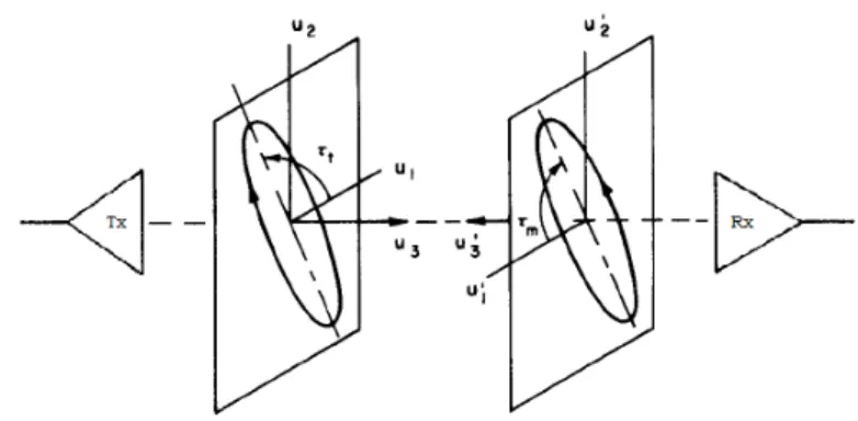
Suppose we have two antennas placed one in a farfield other. Denote by ˆ

ktxthe unit propagation vectors of the wave radiated by the transmitting

antenna and by ˆkrx the unit propagation vectors of the wave radiated by

the receiving antenna, if it placed in transmission. Pr is the total power

radiated from the transmitted antenna and Pdthe power available at the

output section of the receiving antenna, both in input-impedance match-ing. The power Pd depends by the incident power density Sinc= |

⃗ˇ Einc|2

2η ,

by the polarization of the incident wave radiated from the transmitting antenna ⃗ˇp_inc = ⃗ˇEinc

|⃗ˇEinc|

, by source direction of the incident wave ˆktx, namely

by relative orientation between the receiving antenna and the incident wave:

Pd = A(⃗ˇpinc, ˆktx)Sinc (2.1)

(30)

where A(⃗ˇp_inc, ˆktx) is a proportionality constant known as the effective

area.

The effective area of the incident wave can be write as: A(⃗ˇp_inc, ˆktx) = λ2 4πGt(ˆkrx)   ⃗ˇpinc· ⃗p(ˆˇ krx)    2 (2.2) where Gt(ˆkrx) is the receiving antenna gain when it is places in

trans-mission. The term τ = ⃗ˇpinc· ⃗p(ˆˇ krx)    2 (2.3) is said polarization mismatch factor.

The polarization mismatch factor is defined as the ratio of the power actually received by the antenna divided by the power that would be re-ceived from a polarization matched incoming wave. It has value between 0 and 1, if τ = 1 the received power is maximized, while if τ = 0 no power is detect.

Substituting (2.2) into (2.1) and remembering that the incident power density is equal to Sinc= _4πrPr2 Gt(ˆktx) where Gt(ˆktx) is the gain of

trans-mitted antenna, is obtained Pd = Pr  λ 4πr 2 Gt(ˆkrx) Gt(ˆktx) τ (2.4) where _λ

4πr is called free-space loss factor, it takes into account the power

density reduction due to the spherical spreading of the energy radiated by the antenna. For polarization matched antennas oriented in such a way that one is in the direction of maximum gain of the other, and viceversa, the power Pd is maximum and equal to:

Pd = PrG1G2  λ 4πr 2 (2.5)

(31)

25 where τ = 1 and G1 and G2 are the maximum gains.

The use of linear polarized signals can lead to the loss of connection if the transmitting and receiving antennas are orthogonally oriented, the received signal would ideally be zero. This problem can be overcome by using circularly polarized antennas since the polarization factor is independent from the mutual orientation of the two antennas.

A perfectly circularly polarized wave is generated by an antenna that simultaneously excites two linearly polarized wave of equal amplitude and in phase quadrature. Formal definitions for this mode of propagation are given in the IEEE Standard Test Procedures for Antennas[1] _{, where the}

sense of polarization is defined as the sense of rotation of the extremity of the electric field for an observer looking in the propagation direction. Consider the superposition of anx linearly polarized wave with ampli-tude Exand ay linearly polarized wave with amplitude E y, both traveling in the positive z direction. The total electric field can be written as:

⃗

E(z, t) = (Exx + Eyy)e

−jk0z_ejωt _(2.6)

Precisely polarization is the direction of the time-varying real-valued field E(z, t) = Re[ ⃗E(z, t)], at any fixed point z. The corresponding real-valued x and y components are:

Ex(z, t) = A cos(ωt + kz + φa) (2.7)

Ey(z, t) = B cos(ωt − kz + φb) (2.8)

To determine the polarization of the wave, we consider the time-dependence of these fields at some fixed point along the z-axis, say at

(32)

z=0:

Ex(t) = A cos(ωt + φa) (2.9)

Ey(t) = B cos(ωt + φb) (2.10)

The electric field vector ⃗E(t) = Ex(t)x + E y(t)y will be rotating on the xy-plane with angular frequency ω, with its tip tracing, in general, an ellipse. To see this, we expand (2.9) and (2.10) using a trigonometric identity:

Ex(t) = A[cos ωt cos φa− sin ωt sin φa] (2.11)

Ey(t) = B[cos ωt cos φb− sin ωt sin φb] (2.12)

Solving for cos ωt and sin ωt in terms of Ex(t) and Ey(t) we find:

cos ωt cos φ = Ey(t) B sin φa− Ex(t) A sin φb (2.13) sin ωt sin φ = Ey(t) B cos φa− Ex(t) A cos φb (2.14) where we defined the relative phase angle φ = φa− φb.

Forming the sum of the squares of the two equations and using the trigonometric identity sin2ωt + cos2_{ωt = 1 we obtain a quadratic}

equa-tion for the components Ex and Ey, which describes an ellipse on the Ex

and Ey plane: E y(t) B sin φa− Ex(t) A sin φb 2 +Ey(t) B cos φa− Ex(t) A cos φb 2 = sin2φ (2.15) This simplifies into:

E2 x A2 + E2 y B2 − 2 cos φ ExEy AB = sin 2_φ _(2.16)

(33)

2.1. Axial Ratio and XPD 27 To get circular polarization, we set A = B and φ = ±π/2, in this case, the polarization ellipse becomes the equation of a circle:

E2 x A2 + E2 y B2 = 1 (2.17)

2.1 Axial Ratio and XPD

The sense of a circularly polarized wave is determined by the rotation direction of the vector ⃗E as it describes a circle; a right-hand circular polarization (RHCP) signal is generated when the rotation direction is clockwise, while for a left-hand circular polarization (LHCP) wave the vector rotates counterclockwise when the observer is placed in the direc-tion of propagadirec-tion.

For the case φa= 0 and φb = −π/2 we have φ = φa− φb = π/2 and

Ex(t) = A cos ωt (2.18)

Ey(t) = B cos(ωt − π/2) = A sin ωt (2.19)

thus the tip of the electric field vector rotates counterclockwise on the xy-plane then the polarization is left polarized.

Instead for the case φ = −π/2, arising from φa= 0 and φb = π/2, we

have

Ex(t) = A cos ωt (2.20)

Ey(t) = B cos(ωt + π/2) = −A sin ωt (2.21)

thus the tip of the electric field vector rotates clockwise on the xy-plane then the polarization is right polarized.

A practical antenna usually generates an imperfect circularly polar-ized field, therefore the vector traces out an ellipse instead of a circle.

(34)

Figure 2.1: Polarization Ellipse

The spatial orientation of the major to minor axes defines the tilt angle, ψ, in the clockwise direction between a reference position and the major axis looking in the direction of propagation:

tan 2ψ = 2AB

A2_{− B}2A cos φ (2.22)

To provide maximum coupling in point-to-point communication systems the two antennas must be polarization-matched and their tilt angles have to be aligned.

The ratio of the major to minor axes defines the Axial Ratio (AR) of the polarized wave; for perfect CP wave propagation, where only one hand of polarization is generated, the AR will have a value of 1. In the extreme case where the magnitude of the RHCP and LHCP components are the same, the circle formed by the tip of the vector degenerates into a line, the polarization becomes linear, and the AR value becomes infinite. In practical applications, a field is considered circularly polarized when AR is less than 3 dB, however in many applications an AR of 6 dB is

(35)

2.2. Methods to achieve Circular Polarization 29 acceptable.

A real antenna normally generates a desired reference polarization in addition to an undesirable cross-polar component, which is polarized in the opposite hand. In the main beam, the ratio between the power level of the reference wave and the undesirable component is defined such as Cross-Polar Discriminator (XPD) at a given azimuth angle. For a per-fectly circularly polarized pattern, this level is −∞ dB, and for a linearly polarized field, where the two CP signals are of identical magnitude, this level is 0 dB. XPD quantifies the separation between two transmission channels that use different polarization orientations.

The AR is related to cross-polarization by following formula[2] _:

XP D = AR + 1 AR − 1

2

(2.23)

2.2 Methods to achieve Circular

Polariza-tion

For a patch antenna, circular polarization can be obtained if two orthog-onal modes are excited with a 90◦ _{time-phase difference between them.}

This can be achived by modifying the geometry of the patch, by inserting slots, slit or tabs, or by using two o more feeds.

For a rectangular patch the easiest way to achieved circularly polar-ization is to feed the patch at two adjacent edge and for circular patch to feed at two proper angular separation[3] _{, the quadrature phase is}

[2]_{Toh, Cahill, and Fusco, “Understanding and measuring circular polarization”.} [3]_{Richards, Lo, and Harrison, “An improved theory for microstrip antennas and}

(36)

Figure 2.2: Single-feed configuration to obtain CP

obtained by feeding the two feeds with a 90-degree power divider or hy-brid.[4]

To overcome the complexities of dual-feed arrangements, CP can also be achieved with a single feed, in this configurations the principle to obtain the CP is same. The antenna is a diagonally fed nearly square patch, or square patch with stubs and notches along the two opposite edges, or corner-chopped squares, or squares with a diagonal slot. Many others configuration are possible (see figure 2.2).

The dimensions of the patch are modified such that the resonance fre-quencies f1 and f2 of the two orthogonal modes are close to each other.

The antenna is excited at a frequency f0 in between the resonance

fre-quencies of these two modes, such that the magnitude of the two excited modes are equal. Also, the feed-point location is selected in such a way that it excites the two orthogonal modes with phase difference of +45◦

(37)

2.2. Methods to achieve Circular Polarization 31 and −45◦ with respect to the feed point, which results in phase quadra-ture between the two modes.[5][6] _{These two conditions are sufficient to}

yield CP. A similar result is obtained by modifying at the same way a circular or triangular patch configurations with a single feed[7][8][9][10] _.

A further technique to obtain circular polarization consists in exciting the patch by a linear aperture[11][12] _{or by modifying the aperture itself}[13]

located on the ground plane. These techniques, often used in multi-layered structures, have the beneficial effect of increasing the bandwidth. Circular polarization can be obtained also using the sequentially ro-tated array configuration, the single elements could be linearly[14] _or

circularly polarized. In the first case the technique provides that an ar-ray of 2 or 4 patch positioned orthogonally to each other are fed by equal magnitude through a power divider and with a 90◦ mutual phase differ-ence. The performance of the circularly polarized antenna array can be

[5]_{Richards and Lo, “Design and theory of circularly polarized microstrip antennas”.} [6]_{Lo, Engst, and Lee, “Technical memorandum: Simple design formulas for}

circu-larly polarised microstrip antennas”.

[7]_{Iwasaki, “A circularly polarized small-size microstrip antenna with a cross slot”.} [8]_{Wong and Lin, “Circularly polarised microstrip antenna with a tuning stub”.} [9]_{Hsieh, Chen, and Wong, “Single-feed dual-band circularly polarised microstrip}

antenna”.

[10]_{Lu, Tang, and Wong, “Circular polarisation design of a single-feed}

equilateral-triangular microstrip antenna”.

[11]_{Aksun, Chuang, and Lo, “On slot-coupled microstrip antennas and their}

appli-cations to CP operation-theory and experiment”.

[12]_{Huang, Wu, and Wong, “Cross-slot-coupled microstrip antenna and dielectric}

resonator antenna for circular polarization”.

[13]_{Pozar, “A reciprocity method of analysis for printed slot and slot-coupled}

mi-crostrip antennas”.

[14]_{Huang, “A technique for an array to generate circular polarization with linearly}

(38)

increased by using N linearly polarized elements arranged in a circular ring geometry, this N elements are placed at an angle of 360/N degrees with respect to each other and are sequentially fed to generate CP re-sponse. The feed phase of each individual element is arranged in steps of φn = 2π(n − 1)/N where n = 1, 2, ....N .[15] Using circular polarized

patches the technique of sequential rotation allows to improve the purity of polarization and bandwidth[16] _.

2.3 Antenna Measurement

It is usually convenient to perform antenna measurements with the test antenna in its receiving mode because it is assumed that the test antenna can be treated as a passive, linear, and reciprocal device. The ideal con-dition for measuring farfield radiation characteristics is the illumination of test antenna by plane waves: with uniform amplitude and phase. This condition can be approximated by separating the test antenna from the illumination source by a large distance equal to the inner boundary of the farfield region, r > (2D2_/λ)[17]_{. At this distance the curvature of the}

spherical phasefront produced by the source antenna is small over the test antenna aperture but reflections from the ground and nearby object are possible sources of degradation of the test antenna.

A spherical coordinate system can be associated with the antenna under test, see figure 2.3. The antennas coordinate system is typically

[15]_{Teshirogi, Tanaka, and Chujo, “Wideband circularly polarized array antenna with}

sequential rotations and phase shift of elements”.

[16]_{Jazi and Azarmanesh, “Design and implementation of circularly polarised}

mi-crostrip antenna array using a new serial feed sequentially rotated technique”.

(39)

2.3. Antenna Measurement 33 defined with respect to a mechanical reference on the antenna.

Figure 2.3: Standard spherical coordinate system used in antenna measure-ments

There are situations in which the operational antenna illuminates structures in its immediate vicinity; this can modify the radiation field of the isolated antenna. In these cases it may be necessary for measurements of the radiation field to include with the antenna those relevant parts of the nearby structures. The use of scale models is quite common for such cases[18] _.

To completely characterize the radiation field of an antenna, one shall measure its relative amplitude, relative phase, polarization, and the power gain on the surface of a sphere centered where the antenna under test is located. A representation of any of these radiation properties as a function of space coordinates is defined as a radiation pattern.

Since the distance r from the antenna under test to the measuring point is fixed, only the two angular coordinates are variables in a given

(40)

radiation pattern. Usually the operation frequency is treated as a param-eter, with the radiation pattern being measured at specified frequencies. If frequency is varied continuously, such a procedure is called a swept-frequency technique.[19]

A direct method of measuring the radiation pattern of a test antenna is to employ a suitable source antenna, which can be positioned in such a manner that it moves relative to the test antenna along lines of constant θ and constant φ: measurements made with φ as the variable and θ as a fixed parameter are called conical cuts or φ cuts, while those made with θ as the variable and φ as a parameter are called great-circle cuts or θ cuts. Note that the cut for θ = 90◦ is also a great-circle cut. Principal-plane cuts refer to orthogonal great-circle cuts which are through the axis of the test antennas major lobe. For this definition to hold, the beam axis shall lie either in the equator of the spherical coordinate system (θ = 90◦) or at one of the poles (θ = 0◦ or θ = 180◦). Principal plane cuts for linear polarization are usually defined, these would be in the E plane and the H plane of the test antenna.

There are two basic range configurations that accomplish the position requirement for θ and φ cuts. One is the fixed-line-of-sight configuration, here the test antenna and its associated coordinate system are rotated about an axis passing through the phase center of the test antenna. If the test antenna is operating in the receive mode, then the signal that it receives from an appropriately located fixed source antenna is recorded. The other one is called the movable-line-of-sight configuration, for this case the source antenna is moved incrementally or continuously along the circumference of a circle centered approximately at the phase center of the

(41)

2.3. Antenna Measurement 35 antenna under test. If it is moved incrementally, then for each position of the source antenna the test antenna is rotated and the received signal is recorded. Alternatively the test antenna can be rotated incrementally, and for each of its positions the source antenna is moved continuously along its circumferential path.

If the test antenna and the source antenna are both reciprocal de-vices, the functions of receive and transmit may be interchanged. The measured transmitted and received patterns should be identical. In the following, unless otherwise stated, the test antenna shall be considered as the receiving antenna, and it will be illuminated by the field of the transmitting source antenna.

In the case of the fixed-line-of-sight system the θ and φ rotations are provided completely by the positioner for the test antenna. Two positioners which meet the requirements for this system are the azimuth-over-elevation and the elevation-over-azimuth types. These positioners and their associated coordinate systems are shown in figure 2.4.

An example of an elevation-over-azimuth positioner is the Model Tower (see figure 2.5).

(42)

Figure 2.4: Standard positioner configurations and their spherical coordinate Systems

(43)

2.3. Antenna Measurement 37

2.3.1 Gain Measurements

The gain of an antenna is defined as the ratio of its maximum radiation intensity (power flow per unit area) to the maximum radiation intensity of a standard antenna, both antennas being equally energized. In the past, this standard antenna has been a half-wave dipole, but in microwave measurements it has been replaced by a hypothetical antenna which ra-diates uniformly in all directions, i.e., an isotropic radiator. When the gain is compared to that of this isotropic radiator, it is defined as the absolute gain of the antenna.

Two general methods of determining the gain of microwave antennas are possible: Absolute Gain Measurements, and Gain Comparison Measure-ments. The former is usually difficult to perform, so that the one more commonly employed is that of measuring the gain relative to some accu-rately calibrated secondary standard. The absolute gain of this standard antenna, however, must be accurately known, and it is therefore generally determined by the absolute-gain-measuring.

Absolute Gain Measurements

Absolute-gain measurements are based upon the Friis transmission for-mula (see 2.5), which states that for a two-antenna system the power received at a matched load connected to the receiving antenna is given by Pr = PtGtGr  λ 4πr 2 (2.24) where Pr is the power received, Pt is the power accepted by the

(44)

is the power gain of the receiving antenna. This form of the transmission formula implicitly assumes that the antennas are polarization matched for their prescribed orientations and that the separation between the antennas is such that farfield conditions is fulfilled.

The Friis transmission formula can be written in logarithmic form, from which the sum of the gains, in decibels, of the two antennas can be written as: (Gt)dB+ (Gr)dB = 20 log10  4πr λ  + 10 log10  Pr Pt  (2.25) If the two antennas are identical, it follows that their gains are equal so that (Gt)dB = (Gr)dB = 1 2  20 log₁₀ 4πr λ  + 10 log₁₀ Pr Pt  (2.26) The procedure in determining the power gain of the antennas is to measure r, λ, and the ratio Pr

Pt, and then compute the gain of the antenna.

Since two identical antennas are required, this method is referred to as the two-antenna method. If two antennas are not identical, a third antenna is required to determine the gains. For the three-antenna method three sets of measurements are performed using all combinations of three antennas. Three equations, one for each combination, can be written, and each takes the form of (2.24).

The instrumentation required for the measurement of gain using the two-antenna or three-antenna methods shall be highly stable with the source producing a single sinusoidal frequency. it is fundamental cal-ibrate the coupling network between the source and the transmitting antenna so that the power measured at the transmit test point can be accurately related to the power into transmitting antenna. Then all com-ponents of the system are impedance matched using tuners. Finally the

(45)

2.3. Antenna Measurement 39 two antennas are separated so that far-field conditions prevail and bore-sighted so that they are properly aligned and oriented. If the gains of broad-band antennas are to be measured, it may be necessary to use the swept-frequency technique.[20] _{Both the two-antenna and the}

three-antenna methods can be employed.

Gain Comparison Measurements

The gain-comparison measurement, also know the gain-transfer measure-ment, is the method most commonly used to measure the gain of a test antenna. This technique utilizes a gain standard to determine absolute gain and require two sets of measurement. The electromagnetic horn is commonly used for this purpose because of its basic simplicity, reliability, and desirable broad-band impedance characteristics, and because its gain can be calculated from the physical dimensions.

Initially the test antenna is illuminated by a plane wave which is polarization matched to it, and the received power PT is measured into

a matched load, later the test antenna is replaced by a gain standard, leaving all other conditions unchanged, and the receiver power PS is

recorded. From the Friis transmission formula it can be shown that the power gain (GT)dB of the test antenna, in decibels, is given by:

(GT)dB = (GS)dB+ 10 log10

 PT

PS



(2.27)

where (Gs)dB is the power gain of the gain-standard antenna.

One method of achieving this exchange between test and gain-standard antennas is to mount the two antennas back to back on either

(46)

side of the axis of an azimuth positioner. With this configuration the antennas can be switched by a 180◦ rotation of the positioner. Usually absorbing material is required immediately behind the gain standard to reduce reflections in its vicinity which might perturb the illuminating field. Swept-frequency gain-transfer measurements can be performed for testing broad-band antennas. The procedure is essentially the same as that for the swept-frequency absolute-gain measurement, only that the measurement is repeated with the test antenna and the gain standard.

If the test antenna is circularly o elliptically polarized, gain measure-ments can be accomplished by two different methods. One approach is to design a standard gain antenna whit circular or elliptical polarization. In general, the power gains of circularly and elliptically polarized test antennas are measured with the use of linearly polarized gain standards. This is valid because the total power of the wave radiated by an antenna can be separated into two orthogonal linearly polarized components. A single linearly polarized gain standard can be employed and rotated 90◦ to achieve both vertical and horizontal polarizations. Thus the total gain of the circularly or elliptically polarized test antenna can be written as:

(GT)dB = 10 log10

 GT V

GT H



(2.28) where (GT V)dB and (GT H)dB are the partial power gains with respect

to vertical linear polarization and horizontal linear polarization, respec-tively.

2.3.2 Polarization Measurements

In similar manner as for a plane wave, the polarization of an antenna is defined as the curve described by the tip of the instantaneous electric

(47)

Figure 2.6: Polarization Ellipse in Relation to Antenna Coordinate System

field radiated by the antenna in a plane perpendicular to the direction of propagation. This locus is usually an ellipse. Elliptical polarization is characterized by the AR21 _{of the polarization ellipse, the sense of}

rota-tion, and the spatial orientation of the ellipse with respect to a reference direction in the plane containing the ellipse, the tilt angle22_{. For most}

antenna-pattern-measurement situations it is convenient to establish a lo-cal coordinate system in a plane perpendicular to a line drawn between the test antenna and the source antenna, the horizontal axis is usually chosen as the reference direction. Since an antenna usually has a spher-ical coordinate system associated with it, its polarization in a direction (θ, φ) can be illustrated with respect to the coordinate system, as shown figure 2.6.

Also, in order to be consistent with the definition of antenna polar-ization, the local coordinate system associated with each of the waves

21_{see 2.1} 22 _{see 2.22}

(48)

Figure 2.7: Relation between polarization properties of an antenna when transmitting and receiving

is oriented so that one of the coordinates is in the direction of propaga-tion. As a result the tilt angles for the two polarization ellipses, which are measured according to a right-hand rule, are different. As shown in figure 2.7, if τt is the tilt angle for the ellipse described by Et, which is

polarized matched to the receiving antenna, then the one described by Er will be τr= 180◦− τt.

Various techniques are used to determine the polarization of mi-crowave antennas, these can be classified into three categories: Absolute Methods, which yield complete polarization information and require no a prior polarization knowledge or no polarization standard; Comparison Methods, which yield complete polarization information, but require a polarization standard for comparison, and those that yield partial infor-mation about the antennas polarization properties.

The following methods may be employed to measure polarization: • polarization-pattern method

(49)

2.3. Antenna Measurement 43 • rotating-source method

• multiple-amplitude-component method • phase-amplitude method

The polarization-pattern method may be employed to determine the tilt angle and the magnitude of the axial ratio, but it does not determine the sense of polarization. For this measurement the antenna under test can be used in either the receive or the transmit mode. If it is used in the transmit mode, the method consists of the measurement of the relative voltage response |V | of a dipole, or other linearly polarized probe antenna, while it is rotated in a plane normal to the direction of the incident field. The pattern form a figure-eight, as show in figure 2.8, where ψ is the rotation angle of the probe relative to a reference direction. The magnitude |V |, when plotted as a function of the tilt angle τr of the

receiving polarization of the linearly polarized probe antenna, is called a polarization pattern. For an elliptical polarized test antenna, the null of the figure-eight are filled to polarization curve (figure 2.8).

The polarization pattern is tangent with the polarization ellipse of the field at the ends of the major and minor axes. Hence the magnitude of the axial ratio and the tilt angle of the incident wave are determined. The polarization pattern will be a circle if the test antenna is circularly polarized.

The axial ratio (and not the sense of polarization or the tilt angle) can be determined as a function of direction by using the rotating-source method. The method consists of continuously rotating a linearly polarized source antenna while the direction of observation of the test antenna is changed. A pattern of an elliptically polarized antenna obtained by the

(50)

Figure 2.8: Continuously scanned polarization pattern as a function of angle θ

rotating source method is shown in figure 2.9. If the amplitude variations are plotted in decibels, the axial ratio, also in decibels, for any direction in space that is recorded on the pattern is the width of the envelope of the excursions.

The sense of rotation can be determined by performing auxiliary mea-surements. One method requires that the response of two circularly po-larized antenna of opposite hand, one responsive to clockwise and the other to counterclockwise rotation, be compared. The sense of rotation corresponds to the sense of polarization of the antenna with the more intense response.

Another technique is the multiple-amplitude-component method. The test antenna polarization can be determined from the magnitudes of the responses of four sampling antenna having different, but known, tions from the following six choices: horizontal or vertical linear polariza-tion, 45◦ or 135◦ linear polarization, and right-hand or left-hand circular polarization. Usually it is more convenient to measure the magnitudes

(51)

Figure 2.9: Continuously scanned polarization pattern as a function of angle θ

of the linear, diagonal linear, and circular polarization ratios. The axial ratio and the sense of polarization are determined from circular polar-ization ratio since AR = XP D+1_{XP D}₋₁. If the AR is positive the sense is right handed while it is negative the sense is left handed.

In the phase-amplitude method a dual-polarized receiving antenna, linear or circular polarized, is used to sample the field of the antenna under test which is, in this case, used as a transmitting antenna. The outputs of the receiver will be the magnitudes of the responses for each of the polarizations of the sampling antenna and their relative phases. If the two polarizations are orthogonal, the complex polarization ratio can be obtained.

(52)

2.3.3 Anechoic Chamber

An anechoic chamber is a room designed to completely absorb reflections of either sound or electromagnetic waves. They are also insulated from exterior sources of noise. The combination of both aspects means they simulate a quiet open-space of infinite dimension, which is useful when exterior influences would otherwise give false results.

The RF anechoic chamber is typically used to house the equipment for performing measurements of antenna radiation patterns, electromagnetic compatibility (EMC) and radar cross section measurements. Testing can be conducted on full-scale objects, including aircraft, or on scale models where the wavelength of the measuring radiation is scaled in direct proportion to the target size.

The interior surfaces of the RF anechoic chamber are covered with radiation absorbent material (RAM). One of the most effective types of RAM comprises arrays of pyramid shaped pieces, each of which is con-structed from a suitably lossy material. To work effectively, all internal surfaces of the anechoic chamber must be entirely covered with RAM.

Typically pyramidal RAM will comprise a rubberized foam material impregnated with controlled mixtures of carbon and iron, they are in-stalled with the tips pointing inward to the chamber.

The length from base to tip of the pyramid structure is chosen based on the lowest expected frequency and the amount of absorption required. For low frequency damping, this distance is about 60 cm, while high frequency panels are as short as 7-10 cm.

Also, the pyramid shapes are cut at angles that maximize the number of bounces a wave makes within the structure. With each bounce, the wave loses energy to the foam material and thus exits with lower signal

(53)

2.3. Antenna Measurement 47 strength.

There are two basic types of anechoic chambers, the rectangular and the tapered types.

The rectangular anechoic chamber is usually designed to simulate free-space conditions. Even though the sidewalls, floor, and ceiling are covered with absorbing material, significant specular reflections can occur from these surfaces, especially for the case of large angles of incidence. One precaution that can be taken is to limit the angles of incidence to those for which the reflected energy is below the level consistent with the accuracy required for the measurements to be made in the chamber. Often, for high-quality absorbers, this limit is taken to be a range of incidence angles of 0◦ to 70◦ (as measured from the normal to the wall).[23]

The tapered anechoic chamber is designed in the shape of a pyramidal horn that tapers from the small source end to a large rectangular test region. This type of anechoic chamber has two modes of operation. At the lower end of the frequency band for which the chamber is designed it is possible to place the source antenna close enough to the apex of the tapered section so that the reflections from the sidewalls, which con-tribute directly to the field at the test antenna, occur fairly close to the source antenna. Using raytracing techniques, one can show that for a properly located source antenna there is little change in the phase dif-ference between the direct-path and the reflected-path rays at any point in the test region of the tapered chamber. The net effect is that these rays add vectorially in such a manner as to produce a slowly varying spatial interference pattern and hence a relatively smooth illumination amplitude in the test region of the chamber. As the frequency of

(54)

ation is increased, it becomes increasingly difficult to place the source antenna near enough to the apex. A higher gain source antenna is used in order to suppress reflections when this occurs. It is moved away from the apex, and the chamber is then used in the free-space mode similar to the rectangular chamber.[24]

(55)

Chapter 3 Circularly Polarized Antenna

In this section is reported the design, develop, manufacture and experi-mentally validate two simple and efficient solutions for the antenna oper-ating at 5.8 GHz. Either structures are patch antenna which the circular polarization is obtained exciting two orthogonal modes with equal magni-tudes and in phase quadrature. The antennas have been optimized by means of the electromagnetic simulator in order to achieve circular po-larization with Axial Ratio lower than 3 dB at the operating frequency.

3.1 Dedicated Short-Range

Communica-tions Overview

The Dedicated Short-Range Communications (DSRC) is a suite of wire-less standards based on the WiFi architecture, developed mainly by the Institute of Electrical and Electronic Engineers (IEEE), operating in radio frequency in the 5.725 GHz to 5.875 GHz Industrial, Scientific

(56)

and Medical (ISM) band, for communications between Vehicle-to-Vehicle (V2V) e Vehicle-to-Infrastructure (V2I).

Dedicated Short-Range Communications Systems provide a high-speed radio link between Road Side Equipment (RSE), a fixed unit placed on a road infrastructure, and On-Board Equipment/Unit (OBE/OBU), a mobile unit placed inside the vehicle, within a small communication range, up to 1000 meters in optimal weather condition.

In Europe the EN12253 standard[1] _{specifies the requirements for}

the communication between RSE and OBU at 5.8 GHz and the OBU an-tenna features as applicable in the Road Transport and Traffic Telematics (RTTT). The OBU antenna should have a 20 MHz bandwidth (5.795-5.815 GHz) an unidirectional radiation pattern with a main lob width of 70◦ in the vertical plane with the angular EIRP mask suppression of 15 dB, a Cross Polarization Discrimination (XPD) greater than 10 dB in boresight direction and greater than 6 dB within the −3 dB area.

In recent years the OBU market for Electronic Toll Collection (ETC) is rapidly increasing and spreading to several countries, and can be es-timated around 1ML/year due to the large number of OBU devices re-quired. Small size and low cost are the main features for commercially attractive OBU implementation.

For these reasons in the next paragraphs will show two simple and efficient solutions suitable for a OBU antenna of a DSRC system.

[1]_{European Standard EN 12253, Comit´}_{e Europ´}_{een de Normalisation (CEN), Jul.,}

(57)

3.2. Cross-Slot Coupled Patch Antenna 51

3.2 Cross-Slot Coupled Patch Antenna

In this section we will show the study and the experimental characteri-zation of double-layer patch antenna in which the coupling between the feed and the radiating patch is realized through a cross-shaped aperture in the ground plane placed between two layers laminate with the same electromagnetic properties. Appropriately dimensioning the slot sizes and patch lengths left circular polarization is obtained.

3.2.1 Antenna Layout

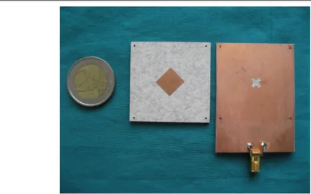
The first antenna structure is designed and realized on Arlon 450, a substrate with relative permittivity ϵr= 4.5 and tan δ = 0.0035.

Ar-lon 450 represents a good alternative to standard FR4, since it has the same permittivity with a very stable behavior at higher frequencies and a better loss tangent. The proposed configuration is a slot-coupled patch antenna, the two substrates have the same permittivity with different height h1 = 0.78 mm and h2 = 1.57 mm, respectively. The antenna has

been designed with total size of 40mm × 40mm × 2.455mm to achieve circular polarization with Axial Ratio lower than 3 dB at 5.8 GHz. The layout antenna is shown in figure 3.1 and the parameters are listed in table 3.1

The 50 Ω feeding microstrip line is placed on the 0.78 mm thick layer, while the radiating patch is realized on the 1.57 mm layer. The microstrip feed line and the slotted ground plane are etched on the oppo-site sides of the first substrate and the feeding structure (strip and slot-ted ground plane) is assembled to be centered below to an almost square patch printed on the second substrate. The common ground plane has a

(58)

w

s

L

2

l

2

l

1

w

f h1 h2

l

f

L

1

Figure 3.1: Antenna layout front and side view. A continuous line is used for the patch, a dashed line for slot in the ground plane, and a dotted line for the 50 Ω feeding microstrip.

cross slot with slightly unequal slot lengths and 45◦ _{inclined with respect}

to the microstrip feed line.

It is known that the resonant frequency of the microstrip patch de-creases with the increasing of the coupling slot length,[2] _{by carefully}

adjusting the lengths of the two arms of the cross-slot the first two reso-nant frequencies of the patch can be achieved with near-equal amplitudes and in phase quadrature. Assuming for simplicity that the patch is per-fectly square the resonant frequency of the resonant mode in the direction perpendicular to the longer slot will be slightly lower than that of the resonant mode in the direction perpendicular to the shorter slot,

(59)

3.2. Cross-Slot Coupled Patch Antenna 53

Table 3.1: Coupled Cross-slot Parameters

Parameter Description Dimension [mm]

S ground plane size 40

ϵr permittivity 4.5

tan δ loss tangent 0.0035

h1 down substrate height 0.78

h2 upper substrate height 0.78

hm metal height 0.035 L1 patch size 9.85 L2 patch size 10.4 l1 slot length 5.4 l2 slot length 5.8 ws slots width 1.7 wf feed length 1.5 lf stub length 3.8

sequently when l1 > l2 a right-hand can be obtained, viceversa, when

l1 < l2 a left-hand CP operation can be achieved.

For ease of fabrication and assembly, the same slotted ground plane has been replicated on the 1.57 mm thick substrate, but the two grounds electrically form a single metal layer. To this regard, for an industrial series production the real final layer stack-up should be considered for fine tuning of CP and some correction steps should be carried out to correctly consider epoxy.

Circularly polarized antennas

Acknowledgment

Contents

Abstract

Chapter 1

Microstrip Antennas

1.1

Advantages and limitations

1.2

Feeding Methods

1.3

Antenna parameters and fundamental

limitations

1.4

Analysis Techniques: an overview

1.4.1

Approximate Models

1.4.2

Numerical Models

1.4.3

Cavity Model

y

2

x

1

3

h

W

4

L

z

ǫ

h

W

L

x

y

z

ǫ

Chapter 2

Circular Polarization

2.1

Axial Ratio and XPD

2.2

Methods to achieve Circular

Polariza-tion

2.3

Antenna Measurement

2.3.1

Gain Measurements

2.3.2

Polarization Measurements

2.3.3

Anechoic Chamber

Chapter 3

Circularly Polarized Antenna

3.1

Dedicated Short-Range

Communica-tions Overview

3.2

Cross-Slot Coupled Patch Antenna

3.2.1

Antenna Layout

w

L

l

l

w

l

L