ELECTRONIC ENGINEERING, AUTOMATION AND CONTROL OF
COMPLEX SYSTEMS ENGINEERING - INTERNATIONAL DOCTORATE XXIV CYCLE
DIEEI
Developing methods and algorithms of sensor
fusion by IMUs applied to service robotics
Coordinator
Prof. Luigi Fortuna Prof. Giovanni Muscato
ELECTRONIC ENGINEERING, AUTOMATION AND CONTROL OF
COMPLEX SYSTEMS ENGINEERING - INTERNATIONAL DOCTORATE XXIV CYCLE
DIEEI
Developing methods and algorithms of sensor fusion
by IMUs applied to service robotics
Coordinator
Prof. Luigi Fortuna
Prof. Giovanni Muscato
OVERVIEW
CHAPTER I – STATE OF THE ART AND INTRODUCTION 1.1 – Inertial Measurement Unit
1.2 – Kalman Filter and Particle Filter 1.3 – Data Filtering
1.4 – Main Hardware: ST-iNEMO IMU Board
[Gyroscopes; Geomagnetic Unit: Accelerometer and Magnetometer; Barometer; Thermometer]
CHAPTER II – ORIENTATION ESTIMATION 2.1 – Introduction
2.2 – Accelerometer Filtering 2.3 – Compass Calibration
2.4 – Method of Orientation Estimation 2.5 – Experiment Result
2.6 – Robot-iNemo interaction results 2.7 – Statistical analysis
CHAPTER III – NAVIGATION AND TRAYECTORY ESTIMATION 3.1 – Sensor fusion algorithm for dead reckoning
3.2 – 3D Navigation: pressure sensor 3.3– Trajectories reconstruction
3.4 – Reconstruction of planar trajectory per vehicle: test 3.5 – Bump detection CONCLUSION ACKNOWLEDGMENTS BIBLIOGRAPHY PUBLICATIONS COURSE/CONFERENCE/PARTNERSHIP
5
I
ABSTRACT
The importance of research in Inertial Navigation Systems (INS) has been growing in recent years. Usually the IMU is used in inertial navigation, such as UAV, AGV, AUV, but it is also used in games, human movement reconstruction (the use of sensors in the studies of human movement is now quickly gaining importance as a promising alternative to video capture systems laboratories), entertainment, etc. Often IMU is used in association with GPS or other sensors to estimate trajectory or for navigation as well as localization. In literature, there are many examples using Kalman Filter or EKF for this aim. It can also be considered to use the implementation of an algorithm in the use of the robot. Moreover, when speaking about an inertial platform there is also a Kalman Filter as a good algorithm providing good results.
The work described concerned the development of systems and algorithms, or new approaches to existing systems to bring robotics to everyday life and to lower costs of implementation of certain devices in industrial processes, or to review some progresses in the light of improvement of technology.
We used the IMUs (Inertial Measurement Unit) and MEMS devices such as accelerometers, gyroscopes, but also temperature and pressure sensors for localization and navigation. Through the use of more accurate sensors and to the growing potential of the new microcontrollers, we have been able to implement algorithms to process and filter data the more quickly and with fewer steps and in some cases to be able to find good solutions at the expense of precision, but in the interest of processing speed.
These sensors have been designed as an aid to existing sensors or for new applications such as three-dimensional localization in a building using
6
the pressure or for safety, in industry, eg for the monitoring of movements of a robotic arm.
Finally, since usually the inertial navigation uses GPS data to correct inertial data, this excludes the GPS spoofing; in other words that someone deliberately alters the signal in such a way that it provides the same values specifically wrong to hack satellite systems installed in the cars.
The IMU used in this work is the iNEMO™ board, an inertial measurement unit developed by STMicroelectronics. It runs a sophisticated sensor fusion algorithm (attitude heading reference system) to provide static and dynamic orientation and inertial measurements. This 10-DOF inertial system integrates five different sensors and has a size of 4x4 cm.
7
OVERVIEW
The purpose of this work of research has been to develop algorithms, methods or new applications for the use of inertial sensors or MEMS (Micro Electro Mechanical System), in order to make less expensive some applications and/or support the traditional systems both for the field of the final consumer - in other words the common man -, and in the field of industrial applications. The importance of research in the inertial navigation systems (INS) has grown in recent years; in fact, usually the IMUs (Inertial Measurement Unit) are used for inertial navigation systems, such as UAV, AGV, AUV; but also for games, for human movement reconstruction, entertainment, etc… IMUs are often used in conjunction with GPS or other sensors to assess the trajectory or the navigation and localization. IMUs usually use MEMS devices, such as accelerometers, gyroscopes, but also Temperature and Pressure Sensors which integrate on-board a firmware that manages the input data. Moreover, each IMU has a suitable algorithm that can be programmed to provide a different output according to the application.
Technological progress has allowed to have sensors more and more at low cost and at a higher level of integration; this progress, combined with the growing possibility of microprocessor calculation - typically integrated directly into the same sensor board - has given the ability to create undefined scenarios for their use (even in areas where previously was unthinkable their use, as for example in the industrial robotics). Starting from the sensors that were kindly provided by the STMicroelectronics worldwide company - with whom there has been a cooperative relationship, and who I thank for the support - several
8
approaches have, therefore, developed whose common theme has been the use of inertial platform to know location, position and orientation of an object, regardless of whether it is a vehicle, a mobile robot or an industrial robot, with particular focus to the application to be implemented.
Undoubtedly basic has been the study of the state of art, and technological advancement considered as initial step, along with the processing of sensor data that could not be taken as raw as they were, but that they had to be treated appropriately, and possibly filtered. The first chapter also highlights that, because the filtering and data analysis introduced the problem of delay, as when using a filter there is always a delay due to filtering and processing. In some cases it has been tried to directly use the raw-data and develop an algorithm that, under certain parameters, could lead to results approximate but fine for our goal.
The work is certainly not directed to the pure research, but to an industrial/business research which could have had an outlet, a job, a policy of continuous cooperation development between research and industry, such as the current Partnership University and ST, which has produced these results. One of these is the development of bump detection that can be useful both for industrial robots and for domestic robots. An example is the robotic vacuum cleaners, now widely used in homes, using the mechanical touch sensors to detect collisions with objects and walls of the room. In place of these accelerometers can be used, as shown in the third chapter, which makes the robot more powerful and reliable both from the structural point of view - because they are less subject to break than the mechanical contact sensors - and also allow implementing on the robot board control other functions by
9
using the same sensor. At the same time in an industrial environment IMUs can be used for estimate and orientation of the robot end-effector, to handle it in an intuitive and simple way.
The first chapter is a brief overview of the techniques studied and tested and the material and hardware used in the development of the algorithms presented. It also refers to the importance of filtering and data analysis and their correction.
The second chapter examines in detail the algorithm developed to guide an industrial robot using inertial platform. Usually to move such a robot it is necessary to define a system of coordinates, the end point of the robot tool, and in which trajectory we want to move it. The robot is programmed in the control unit by qualified personnel and then started up, the robot will do the same thing a million times in the same way, with a very high degree of accuracy in repeatability. Thinking now to replace the encoders with the IMUs on the links at the current state of MEMS technology is unthinkable because we would have not the same degree of precision or repeatability with the degree of tenths of a millimetre that they have (even if there is already a patent in this sense). What has been done instead, in collaboration with Eng. Giacomo Spampinato at Malarden University in Sweden, is to have an easier use of the robot; in fact we can use the IMU the same way as a joystick, so that any worker not in possess of an advanced training could use it easily and intuitively. Another use of the IMU in industrial robotics may be directed to safety in the workplace and in workings. Using statistical analysis we can see if there is an abnormal function of the robot. In fact, by placing one or more inertial platforms on the links and on the end-effector, it can be determined whether during their movement there is a different behavior
10
than expected. The implementation of this feature would allow, by using a safety routine, to stop the robot immediately in the event that it impacts an object, or for a technical problem, or for the failure of some component. So we tried to have a multilateral vision of the types of problems to be addressed to: with similar algorithms or methodologies we can face and solve different problems in different fields and applications, and also find new ones.
Finally in the third chapter we go back to use the GPS with inertial platforms. Also in this case alternatives for the correction of errors develop independently and we attempt to assess the reliability of the GPS itself. Again, we look at the applications and industrial developments, such as many insurance companies now use the GPS to quantify the number of kilometres per year, and thereby allowing to know the risks associated with that customer and how much has to pay, or it is often installed as anti-theft tracking device. Unfortunately there is already a countermeasure, there are devices that simulate a GPS signal of excellent quality, shielding the correct signal to the receiver and making believe that the car stopped at one point or it is on a trajectory that is actually different from the real one. In this sense we can understand the usefulness of the reconstruction of the path travelled by a vehicle using only the inertial platform to a level that ensures also how measured by GPS.
In conclusion we tried to use an inertial platform and MEMS sensors, developing new approaches to solve old problems, and new methods to face current issues. Moreover, new algorithms and solutions and/or simplifications of the old ones were designed, so as to permit their use economically, efficiently and functionally in the domestic and industrial
11
applications, in the perspective of interaction and integration between research and industry from which both could receive benefit.
13
CHAPTER I - STATE OF ART AND INTRODUCTION
1.1 INERTIAL MEASUREMENT UNIT
The localization of an object inside a space, internal or external, is a problem under continuous evolution which, during the last years has known an exponential development of its applications and used methodologies. The growing availability of low-cost sensors has made easier the approach to this issue, driving research towards innovation of methodologies of sensor fusion. Being able to make use of information deriving from different sensors shows the value of any more precise and accurate magnitude. This combined with the increasing reduction in the size of the available sensors has led to the development of applications designed to be integrated into any mobile device. Devices such as accelerometers or gyroscopes have become part of common language and have aggressively invaded any device on the market, finding space even on platforms whose use until a few years ago was unthinkable. We can clearly see, therefore, how important is to maximize in parallel these devices’ performance and potentialities. On the other hand, the use of more sensors for the valuation of any physical quantity, as well as being complex in the computational and theoretical point of view, it results to have not few difficulties with the their integration into a single platform. It would be sufficient to note that each sensor has a consumption of energy which, as much as we could optimize it, it shall affect the duration of an independent power system embedded proportionally to the number of actual sensors. Moreover, the chance to obtain accurate valuations through low cost sensors without the aid of more sophisticated sensors
14
(and therefore more expensive) is undoubtedly attractive and has provided a great boost to the optimization of applications to this sense. On this point of view the developed work lies, and what will be outlined below. Through special mathematical tricks we tried to rebuild at the best the information deriving from an inertial sensor platform provided by ST Microelectronics, refining them as much as possible, in order to derive an estimate of position using the fewest possible sensors. For example using only the accelerometer data it is possible to rebuild the position of objects and / or obstacles in a room, using it as a "bump sensor" and then doing SLAM.
An IMU applied to a body provides output data related to the various dynamic measured magnitudes: linear and angular accelerations, magnetometer data, but also temperature, pressure, etc. The development of these quantities, joint with the knowledge of GPS coordinates allows us to reconstruct the movement of the body, with a better accuracy respect to that given by the single GPS, even when the fix of this is not always available.
The use of inertial sensors into aircraft or land vehicles is nowadays a great used resource, especially for purposes of direct georeferencing or mobile mapping in the LIDAR and, more generally in the field of geodetic survey. The growing use of these sensors, combined with the development of existing satellite constellations (GPS and GLONASS), to the next appearance of the European Galileo system, and to the possible application of modern means of treatment and estimation of signals (eg the Kalman filter), all them get to guide industrial research on their use in personal and low cost navigation applications.
15
In the past years along with the research activity an integrated software environment has been designed and developed for processing the output data from the IMU ST, iNEMOTM with the obtained information from the navigation sensor GPS TESEO STA8058 EVB Rev. 03; in order to obtain accurate information on the positioning of the vehicle where the system is installed on. The above said vehicle we can imagine being able to rebuild the path flown without human aid. Many of the activities here described have been carried out at the IMS Systems Labs of STMicroelectronics in Catania as well as in the laboratories of the University of Catania DIEE.
1.2 KALMAN FILTER AND PARTICLE FILTER
The Kalman filter is an efficient recursive filter that evaluates the state of a dynamic system from a series of measures subjected to noise. For its intrinsic characteristics it is a great filter for noise and disturbances acting on the system zero-mean Gaussian. It is used as an observer state, such as loop transfer recovery (LTR) and as a parameter identification system. The filter gets its name from Rudolf E. Kalman, although Thorvald Nicolai Thiele and Peter Swerling actually developed a similar algorithm before. Stanley Schmidt is generally recognized to have been the first to develop a practical implementation of a Kalman filter. This was during a visit by Kalman to the NASA Ames Research Center, during which Schmidt saw the applicability of the Kalman’s ideas to the problem of estimation of trajectories for the Apollo program, ending with including the program on the Apollo on-board computer. The filter was developed in scientific articles by Swerling (1958), Kalman (1960) and Kalman and Bucy (1961).
16
Several types of Kalman filter were subsequently developed, starting from the original formulation of Kalman, now called the Kalman easy filter; some examples are the extended filter by Schmidt, the information filter and various square root filters developed by Bierman, Thornton and many others. It can be considered a Kalman filter also the phase-locked loop (or PLL), an electronic circuit now used in countless applications, from radio broadcast to computers, from data transmission to sensor fusion.
The Kalman filter uses the dynamic model of a system (for example, the physical laws of motion), known control inputs and system measures (eg from sensors), to make an assess of the variable quantities of the system (its State) which is better than the assess obtained by making a single measurement.
All measurements and calculations based on models are to a certain extent, estimates. Noise in sensor data, approximations in the equations that describe how to change the system and external factors that are not taken into account, introduce some uncertainty on the deduction of the values of the state of a system. The Kalman filter mediates the state of a system with a new measure using a weighted average. The purpose of the introduction of the weights is that the values with a better (ie smaller) uncertainty estimated are "trusted". The weights are calculated from the covariance, a measure of uncertainty (estimated) on the prediction of the system state. The weighted average result is a the new estimate of the state that lies between prediction and measurement of the state, and, therefore, it is a better estimate. This process is repeated for each step, with the new estimate (and its covariance) used for the next iteration of the prediction. Then the Kalman filter operates recursively and considers
17
only the "best guess" - not the whole story – of the state of a system to calculate the next state
When the actual computation for the filter is performed, the state estimate and covariance are coded on matrices to manage the multiple dimensions involved using mathematics known on matrix calculus. Generally it is preferred writing the Kalman filter distinguishing two distinct phases: prediction and update.
The prediction step uses the state estimate of the previous time step to produce a state estimate at the current time step. This state estimate is also known as the a priori estimate because, although it is a state estimate at the current time step, it does not include information for measuring the current time step. During the upgrade, the current a priori forecast is combined with information of the current measure to refine the assessment of the state. This best estimate is called the a posteriori state estimate.
In general, the two phases are alternate, with the expectation of state advancement to the next planned measurement and the update incorporating this measure. However, this is not necessary, if the measure is not available for some reason, the update phase may be ignored and only predictions can be run. Likewise, if several independent measurements are available at the same time, several phases of renovation can be made (usually with different observation matrices Hk).
Prediction phase State estimation a priori
18 Update
Innovation or measurement residual
Innovation or covariance residual
Kalman excellent gain
Updated estimation of the a posteriori state
Updated estimation of the a posteriori covariance
This formula for the estimation of the state and covariance update only applies for the Kalman gain.
Within the representation of the localization, the particle representation has a set of advantages: we can use the sensory characteristics, motor dynamics, and arbitrary distributions of noise. These are universal functions which approximate the equation for the probability density, which can overcome very restrictive assumptions than other approaches, focus computational resources in most relevant areas by sampling in proportion to a posteriori density.
Creating a software algorithm implementing them is quite simple. The use of particle filters is due to the difficulty of effectively representing relationships describing the system in all its features. The use of pure probabilistic filters requires the knowledge of the probability density function form, which are often extremely complex and defined on a
19
multidimensional domain. In order that the particle approach results in a viable option, we should consider that: the choice of the proposal function is crucial for the generation of probability functions; a large number of samples causes more computational power absorption; the samples can degenerate if one of them assumes a much greater weight than others and this would cause a loss of diversity that would weaken the algorithm.
After building the system and perceptual models, it becomes possible making the special particle filter for the application we should implement. Particularly the distribution to be made must allow predicting the next state by starting from the current state. In this case having an estimate which takes into account, not only controls, but also observations, would increase our chances of success. This kind of feature is as powerful as difficult to create: finding a mathematical function that intersects the observable and controllable system parts is very complex. The solution, as for the perception model, might be algorithmic. In this case, however, the development could not be off-line, as the position estimates are one of the steps of the localization cycle, so they must be done frequently and in real time.
While the values of the sensors can be queried only when you must assign a weight to the particle filter samples, it is essential to access the sensor values with a very high frequency: the predictor step in the tracking algorithm is based on the robot translational and rotational speed. If these values are not correct, particle can follow completely wrong trajectories.
20
The particle filter has been introduced for the application of spoofing GPS, where an attempt was made to have a reliability of the GPS through the use of the inertial platform.
1.3 DATA FILTERING
An INS, Inertial Navigation System, is basically a calculator estimating the position of a vehicle compared to a known system, based on measurements of a set of sensors installed on the vehicle. Independence from external structures (eg. Satellites) ensures continuity on position tracking. The used sensors as inertial navigation system are accelerometers, acceleration detectors along a specific direction, and gyroscopes, measuring the rotation speed. The measuring unit consists of a triad of accelerometers and one of gyroscopes arranged in according to an orthogonal system. By integrating the acceleration and rotation components, position and current layout of the body are calculated. The INS systems require knowledge of data such as position and layout starting and proceed by integrating the differential equations of motion (Equations of navigation).
However, this approach is affected by a large error component due to sensors drift, which, accumulated over time, lead to an overall degradation of the position estimate. For this reason, inertial navigation systems have been integrated with external sources, such ass the GPS through the use of various sensor fusion techniques.
The most effective and best known of these is the one which integrates information from the GPS with the equations of motion characterized by sensorial data through the use of a special Kalman filter.
21
This approach, as much as accurate and satisfactory is, however, it leaves unresolved the issues related to navigation in environments where the signal is not available. Hence the need to develop new techniques that make the estimation of position in these cases more accurate and fast. For the estimate of the position of an object in space starting from measurements provided by the inertial sensors, it is necessary to digress on position body estimate subject to a one-way motion from information on accelerations impressed on it.
This seemingly trivial problem is complicated significantly by the presence of any error which can not be compensated directly or indirectly through information from other sensors.
The worst case is the use of a single sensor for the estimation of a position in the space because it is subject to large and growing percentage of error, which increasing the time cause increasing uncertainty to spatial location of the object that you want to estimate the position. In a very general way, we can say that the speed of an object subject to an acceleration a(t) in the interval (t-t0) and having an initial
speed v0 is given by:
Once obtained the speed, the position at time t is given by:
by replacing the speed value obtained in the first equation, in the expression on the position we get:
22
Looking at the above expression we note how the position from moment to moment depends on an integral double of acceleration. This simple but effective observation highlights how each error in measuring acceleration from any sensor is integrated twice and propagated in time greatly and irreparably impairing the final estimate of the position of the object. The errors that are subject to the acceleration measurements carried out with MEMS-type accelerometers are well known in the literature. These are mainly due to the following types:
1. Dynamic and highly variable bias over time 2. White noise overlapping the output signal
3. Juxtaposing of components of the gravitational acceleration with the signal
4. Oscillations in the absence of external stimuli, too
It seems so obvious how the integration of raw data from the accelerometer, gyroscope and other MEMS is totally inadequate for the estimation of the location or development of any navigation algorithm. The adoption of appropriate mathematical tools can solve this problem in part by offering some alternatives to sensor fusion.
To adequately understand the extent of drift that is subject the estimate of the position performed through a signal subject to a random type of inconvenience (white noise with Gaussian distribution), it is sufficient to make a proper numerical simulation in Matlab® - a program of numerical calculation produced by Mathworks which can provide a wide range of functions and tools for the representation and manipulation of time series, and any type of system. Such step, however apparently superfluous, allows a clear view of what should be the response of our
23
system to estimate a specific impulse and what is actually the reply received.
First you need to model the dynamics of the system, this can be easily done using the canonical form of state of a discrete linear system of the type:
In the particular case just start from the physical laws that govern the dynamics of the body in the event of uniformly accelerated motion:
Bringing all in matrix form and rewriting the system in discrete form we get:
This simple form represents our system composed by state variables coinciding with position and speed at time k +1 commanded from the input U coinciding with the acceleration at time k. Transcribing the system under consideration in Matlab and providing undisturbed acceleration we can see the correct behavior of the system. For example, by imposing an acceleration with a sinusoidal pattern described in figure:
24 0 200 400 600 800 1000 1200 -1 -0.8 -0.6 -0.4 -0.2 0 0.2 0.4 0.6 0.8 1 Number Of Sample A c c e le ra ti o n Noiseless Acceleration
Figure 1. Example of unperturbed input
A similar input produces the following output:
0 200 400 600 800 1000 1200 -1 0 1 A c c e le ra ti o n 0 200 400 600 800 1000 1200 -20 -10 0 10 V e lo c it y 0 200 400 600 800 1000 1200 -1000 -500 0 Number Of Samples P o s it io n
Figure 2. Response of the system to the unperturbed input
By a brief visual analysis is shown how the application of a sinusoidal acceleration produces a variation of speed to be brought back to zero after a whole period of the input sinusoid; this implies a total body move
25
that may be certified to a constant value over time at the end of the application of the acceleration signal of sinusoidal.
To understand how a signal affected by noise during acceleration goes to affect the estimate of the position in the system under investigation, we must produce a signal similar to the previous one, which is overlapped from a white undisrupted noise, and use it as input, as done with the undisrupted signal. If we proceed thus disrupting the sinusoid input lightly with a white noise variance 0.2m/s2, we obtain the following result: 0 200 400 600 800 1000 1200 -1 -0.5 0 0.5 1 1.5 Number Of Samples A c c e le ra ti o n
Figure 3. Example of input perturbed by Gaussian white noise This produces in output:
26 0 200 400 600 800 1000 1200 -1 0 1 2 A c c e le ra ti o n 0 200 400 600 800 1000 1200 -20 0 20 40 V e lo c it y 0 200 400 600 800 1000 1200 -500 0 500 1000 P o s it io n Number Of Samples
Figure 4. Response of the system to the perturbed input
As we can easily imagine the noise introduced by the previous figure has produced a drift speed the system which leads to the detection of a shift that does not exist. This is even clearer by comparing individual velocities and positions in absence of noise (true velocity) and in presence of noise (Measured velocity):
27 0 200 400 600 800 1000 1200 -20 -15 -10 -5 0 5 10 15 20 25 Number Of Samples V e lo c it y true velocity measured velocity 0 200 400 600 800 1000 1200 -800 -600 -400 -200 0 200 400 600 800 Number Of Samples P o s it io n true position measured position
Figure 5. Comparison between the system outputs at the presence of noisy and not noisy input
28
It is, therefore, needed a digital filtering of the input data allowing to remove more accurately as possible the noise overlapping the signal. In this sense, there are several possibilities producing significantly different results in terms of computational burden and, hence, the time taken to reconstruct the signal. The time parameter in applications - as real-time - becomes a key discriminator in order to make the correct choice and the more appropriate filtering method. Below are some types of filters that can be applied to this examined case in order to reconstruct the original signal. As we shall see later digital filtering is closely related to the methodology for data integration.
The first type of filter under exam belongs to the family of FIR filters, they are also named moving average since their output is simply a sort of weighted average of input values.
These filters present the major drawback of approximating the ideal filter perfectly only for very large values of N, tending infinite. This means they have a very high computational cost because for each sample input, N multiplications and N additions must be calculated, which makes unattractive the use of FIR filters in real-time applications.
In its simplest form a moving average filter is the following relation:
By applying this simple iteration to a perturbed signal we get a result with accuracy increasing proportionally to the number of samples used.
29
Figure 6 Examples of moving average digital filtering
This method, no matter how simple, has many drawbacks due to the increasing phase delay output of the filter at the growing of the used samples and to the extensive computational operations necessary to perform all the filtering. An excellent alternative to the methodology above is provided by the SMOOTHING of the data in a progressive manner. It is also in this case a moving average filter, but reformulated in order to clear the phase delay and reduce the computational order. The smoothing, however, must be performed several times in order to be effective, but on the other hand, the number of steps necessary for its "convergence" appear to be relatively few.
In Matlab has already implemented a smoothing function that allows filtering the data with the following methods:
30
Figure 7. Summary table of the types of filtering in MATLAB
The various methods differ depending on the weights assigned to the different coefficients of regression and shall be selected depending on the nature of the disorder. By applying a filter with a window of samples of variable amplitude at 51 'lowess' mode we obtain the following result, which already has a good filtration on the first iteration:
0 200 400 600 800 1000 1200 -1 -0.5 0 0.5 1 1.5 Number Of Samples A c c e le ra ti o n noisy data filter data
31
Once chosen the method of filtering of the data it necessary to proceed to choose an appropriate integration methodology.
In the presence of discrete data such as those provided by a sensor after each sampling interval T, to proceed to their integration you need to apply the concepts and tools described in the mathematical theory of numerical integration. The numerical integration is strongly bound to the type of interpolating polynomial, from which it can not be separated. In general, using numerical integration algorithms which allow us to integrate functions whose are not known the analytical expression but only a few values at certain moments. The formulas of numerical integration (or quadrature) are approximation algorithms of the integral obtained by the integration approximation of the integrand.
The problem then is to approximate as accurately as possible the integral:
∫
=
ℑ
b adx
)
x
(
f
where f(x) is a function continuing in [a,b]. The integration formula will be such:
∑
= +=
n i i i nw
f
x
I
0 1(
)
where x0,x1,K,xn are named bonds and w0,w1,K,wn weights.
The difference between the integral in analytical form and its numerical approximation is called the rest and represents the analytical error in the approximation of the integral that is committed:
32 1 1 + + =ℑ− n n I r
This error depends strictly on the number of knots chosen to evaluate the integral. In relation to this the numerical approximation of the integral is called of level of precision p if for f(x) = xi, i =0,1,K,p the rest is null, while for f(x) = xp+1 it is different from zero.
Considering the polynomial interpolation of f (x) written in the form of Lagrange:
and hence considering the integral of Ln(x) instead of f(x), we obtain:
Where wi are the weights for the approximation formula given by:
. , , , ) ( , x dx i 01 n l w b a i n i =
∫
= KThese weights can be determined by requiring that the has no level of precision n. In other words, they can be determined by solving the following system of equations:
+ − = + + + − = + + + − = + + + + + . 1 n a b x w x w x w 2 a b x w x w x w a b w w w 1 n 1 n n n n n 1 1 n 0 0 2 2 n n 1 1 0 0 n 1 0 K M K K
33
The matrix of the previous system, called Vandermonde, is not degenerate, so the system has one and only one solution. If
n 1
0,w , ,w
w K
is the solution of the system, the quadrature formula:
∑
= + = n 0 i i i 1 n w f x I ( )has a degree of precision almost n.
There are several types of numerical integration all turned to minimize the analytical error of the integral calculus, these can be attributed to two main categories:
Newton-Cotes formulas: in which knots are set in the interval [a, b] and are equally spaced. These formulas have no level of precision n or n +1 and their weights are easily obtainable and can be expressed by simple rational numbers. This approach has the handicap of presenting weights of variable sign for n> 9.
Gaussian formulas: knots are not prefixed in advance, but with the weights they are derived to maximize the degree of accuracy that results 2n +1. These formulas, as compared to those of Newton-cotes, have the advantage, in addition to the high degree of accuracy, to have the weights always positive but at the price that the expression of the knots and the weights, is often not rational.
We have chosen to use the Gaussian formulas since they maximize the precision of the integral, and being the interpolating function fixed a priori, it is possible to calculate the off-line weights and knots and putting them in real-time in the approximation formula without further resource waste. In particular the algorithm of integration to which we will refer is
34
the Gauss-Legendre. The following definitions and theorems are the basis of the algorithm chosen, and allow to understand the mathematical concepts adopted in the development of the integration method of Gauss-Legendre.
Definition: A vector space Γ of the real field R, which is called a scalar product, is called Hilbert space if every Cauchy sequence of elements of Γ is convergent.
Definition: Given a weight function w(x) not negative in the interval (finite or infinite) (a, b) and not identically null and a set of polynomials , where is of degree i, it is a Hilbert space respect to the scalar product:
Definition: A polynomial system is called orthogonal respect to a weight function w(x) and to the scalar product defined above if:
The interval (a,b) and the weight function w(x) univocally define polynomials pi less than non-null constant factors.
Theorem: For every n>0, the orthogonal polynomial has n zeros real or distinct and all contained in (a,b). Furthermore, the zeros of alternate with those of ie between two consecutive zeros only one zero exists of .
Theorem: A quadrature formula of interpolatory type built on n+1 points has degree of precision at least n and at most 2n+1. The maximum level
35
is reached if, and only if, the knots are the zeros of (n+1)-th orthogonal polynomial to the weight function w(x) = 1.
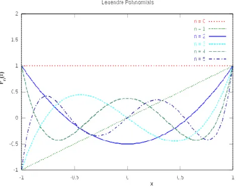
The orthogonal polynomials that are used in the case of Gauss-Legendre formulas are precisely the Legendre polynomials. They are defined as solutions of the differential equation of Legendre:
The Legendre differential equation can be solved by standard methods of power series. We have solutions given by convergent series for |x| <1. We have also converged solutions for x = ± 1 provided that n is a natural whole (n = 0, 1, 2, ...) in this case the solution of changing of n form a polynomial sequence called "Succession of Legendre polynomials". They can therefore be defined for recurrence according to the formula:
36
Figure 9. Performance of Legendre polynomials up to the fifth degree
These polynomials are also useful for very precise calculation of a polynomial of discrete values of the accelerations.
After defining the Legendre polynomials the Gauss quadrature formula can be easily obtained, assuming we want to integrate the function with n+1 knots, performing the following steps:
Calculating the Legendre polynomial p of degree n+1, to compute xn
nodes.
Calculation of Legendre polynomial q of degree n+2, to calculate the weights using the formula:
37
The so calculated weights and nodes will be defined in the interval [-1,1], then I carry them to the interval [a b], with the transformation:
Finally, we apply:
Where, we remind, f(x) is the interpolating function to be determined. A crucial step for a successful integration of any discrete data is a precise and consistent interpolation. There are again various types of interpolation, the use of which is discriminated by the type of precision that we want to get.
The problem, quite generally, can be defined as follows:
Given a sequence of n distinct set of real numbers xk called knots, and for each of these xk gave a second number yk. We aim to find a function f such that the relation is satisfied:
Where n represents the number of samples available to us.
We therefore speak of: known some data pairs (x, y) interpretable as points of a plan, we aim to build a function, called interpolating function, which is able to describe the relationship between the set of values x and the y values ensemble.
38
A first and obvious example of interpolation is the linear one, in which for every pair of consecutive points called (x, y) and (xb, yb) is defined interpolating function in the range xa, xb the following function:
This interpolation produces a response like:
Figure 10. Example of linear interpolation
This type of interpolation is very fast and basic, but it has several handicaps, such as the discontinuity in the transition points and an error increasing with the square of the distance of the points to be interpolated. More precise and complex respect to the linear interpolation is the polynominal, which can be regarded as a generalization of the previous one, and that is to approach the interpolating function with a polynomial of degree n by using the method of least squares. Since, for example, a
39
set of discrete data that you want to interpolate with a polynomial of degree n such as:
And given a set of m samples, with m ≥ n, we will interpolate the data as:
By naming with B the matrix constituted by samples xm, with the
coefficient vector and Y the sample vector corresponding to each xm, we
will get that the coefficient vector is given by:
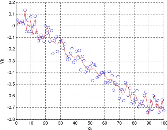
To make the most accurate polynomial approximation can be thought of dividing the interval into subintervals of interpolation to be interpolated separately, this will make more accurate the result but it will introduce points of discontinuity between a set of samples and the other. By applying this method to a set of points where a white noise is superimposed, we obtain for example:
40 0 10 20 30 40 50 60 70 80 90 100 -0.8 -0.7 -0.6 -0.5 -0.4 -0.3 -0.2 -0.1 0 0.1 0.2 Xk Y k
Figure 11. Example of polynomial interpolation
Using a fourth-degree polynomial interpolation. A big problem with this approximation is that it suffers from Runge's phenomenon. The Runge's phenomenon is a problem related to the polynomial interpolation of high degree polymonials, it is the progressive increasing of the error near the ends of the range as shown in the below figure:
41
The red curve is the Runge function, the blue curve is a polynomial of the fifth degree, and the green curve is a polynomial of ninth degree. Ordinate we have the error, as you can see the approximation deteriorates with increasing degree. In particular, interpolation by a polynomial Pn(x) of degree n, it gets worse according to the relation:
To overcome this problem and does not affect further the integration of data with additional errors caused by interpolation it has been chosen to use another technique called cubic spline interpolation. This methodology is a particularization of the method of spline function interpolation.
A spline function is defined in the following way:
given as a closed interval subdivision [a,b]. A spline function of degree p with knots at the points xi with i=1,2, ... n is a function on [a,b] denoted by sp(x) such that, in the interval [a,b] we have:
in each subinterval [xi,xi+1] where i=1,2,…n the function sp(x) is a
polynomial p degree the function sp(x) and its first derived p-1 are continuous in each sub-interval.
Particularly, the natural cubic spline function is nothing more than a spline function of third degree. The idea behind this interpolation is to divide the samples interval into smaller intervals interpolated by an appropriate spline.
42
Use a third-degree polynomial with continuous derivative in each sub-interval can correctly interpolate any signal getting significantly better results compared to a polynomial interpolation.
The application of this type of interpolation to the previous case we obtain: 0 10 20 30 40 50 60 70 80 90 100 -0.8 -0.7 -0.6 -0.5 -0.4 -0.3 -0.2 -0.1 0 0.1 0.2 Xk Y k
Figure 13. Example of cubic spline interpolation
You can see how, even in presence of a highly variable signal, this solution produces much more satisfactory results than those of the linear interpolation.
The interpolation polynomials of Legendre polynomial is similar to that based on the method of least squares, but due to the nature of the interpolating polynomials it can approximate to a finely discrete signal even in presence of a strong variation of that.
Unfortunately a large computational burden is required due to the high number of Legendre polynomials to use; but it does not suffers from
43
Runge's phenomenon and can be used in off-line data processing. The interpolation formula in this case is the following:
Where the various P(x) in this case are the Legendre polynomials previously defined and which can be tabulated before the interpolation itself. In relation to the previous case, this interpolation provides a slightly better (but takes longer) result than the natural cubic spline:
0 10 20 30 40 50 60 70 80 90 100 -0.8 -0.7 -0.6 -0.5 -0.4 -0.3 -0.2 -0.1 0 0.1 0.2 Y k Xk
44
1.4 MAIN HARDWARE: ST-iNEMO IMU BOARD
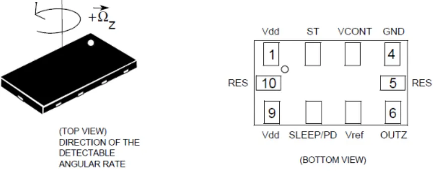
The sensor platform used primarily for the development and the work presented is a prototype provided by ST (STEVAL-MKI062V1) called the iNEMO™; that is, iNErtial MOviment unit. Actually to this, time to time, it has been developed alongside other boards such as CRM003 GPS board, equipped with Theseus chip, connected to the iNEMO gate UART2 through a level translator ST3232, or the rover I.A.F.F.I.E.D.D.U. developed on control cards based on microprocessor STM32 which is of ARM model.
The iNEMO inertial platform, developed by STMicroelectronics, is a 10-axis Inertial Measurement Unit (dof, degrees of freedom), made with:
- 6-axis geomagnetic sensor, LSM303DLH: 3-axis accelerometer and 3 axis magnetometer. Digital output with protocol I2C - 2-axis gyroscope (roll, pitch), LPR430AL, analog output - Axis yaw gyroscope: LY330ALH, analog output
- Pressure sensor LPS001DL, a digital output with protocol I2C - STLM75 temperature sensor, a digital output with protocol I2C - MCU Microcontroller Unit STM32F103RE
The board shows various options for interfacing: MicroSD card connector (data logging), USB connector, serial connector and a connector for an optional wireless interface.
It is an inertial system to 10 degrees of freedom which can be used in many applications such as, for example, virtual reality, augmented reality, image stabilization in a camera, man-machine interaction and robotics.
45
Figure 15. STEVAL-MKI062V2, iNEMO, realized by STMicroelectronics, Catania
The firmware supplied with the board has an integrated sensor fusion algorithm AHRS (Attitude and Heading Reference System) that provides an output roll, pitch and yaw (roll, pitch and yaw, in the notation of Euler angles, explained graphically in the below figure) and the parameters q0,
q1, q2, q3 on the notation with quaternions
.
Figure 16. Graphical explanation of the angles of roll (rotation around the X axis), pitch (rotation about the Y axis) and yaw (rotation around the Z
46 Gyroscopes
Figure 17. Roll and pitch gyroscope: LPR430AL: 2-axis gyro (roll, pitch) 300°/s full-scale
Figure 18. Giroscope yaw: LY330ALH: yaw-axis gyro 300°/s full scale
iNEMO uses two devices to detect the angular velocities around the three axes: LPR430AL in the same package contains two gyroscopes that detect the speed of rotation around the axis of rolling and pitching; LY330ALH detects the speed of rotation around the yaw axis. The output of the gyroscopes is analog, connected to an ADC, present in the same microcontroller.
47
Geomagnetic Unit: accelerometer and magnetometer
Figure 19. Geomagnetic module LSM303DLH: 6-axis geomagnetic module
The geomagnetic module LSM303DLH in the same package integrates a three-axis accelerometer and a three-axis magnetometer. It is interfaced with the microcontroller via I2C interface.
Barometer
Figure 20. LPS001DL: pressure sensor 300-1100 mbar absolute full scale
The pressure sensor measures the air pressure LPS001DL in the range 300-1100 mbar. It is interfaced with the microcontroller via I2C
48
interface, it is a high-resolution sensor. The sensing element is based on a membrane with a piezoresistive approach and proper conditioning electronics based on a Wheatstone bridge and amplifiers, it converts pressure into an electrical signal. The sensor also features two programmable interrupts to recalibrate and adapt it to different pressure events, not only, we have also a DRS interrupt (data ready signal) which is also managed by micro, which provides better data synchronization. The following circuit shows the micro outputs to manage INT1 and INT2.
Figure 21. Pressure sensor schematic
Thermometer
49
The temperature sensor STLM75 detects the environmental temperature in the range from -55°C to +125°C. It is interfaced with the microcontroller via I2C interface.
Along with the Hardware, the DLL libraries have been developed and made available by ST where the necessary functions are implemented to interface of the board with Matlab or other development environments. DLLs also provide communication with GUI iNEMO, an intuitive graphical interface shown in the following figure; it is useful to be able to become familiar with the signals from the sensors and display them on screen in a simple and immediate way. This aspect is not of secondary importance in understanding the nature of the signals work, the noise to which they are affected is an important first step to begin to understand which could be the first steps of developing an algorithm, for example: the filtering data, the correction of off-set, the correction of over-elongations and settling times typical of MEMS structures.
50
The interface allows to display information from sensors either continuously or for a finite number of samples, but also to save them as files “*.tsv”, enabling you to load data into calculation software such as Matlab and set so the development of algorithms off-Line.
The connection between the board GPS and iNEMO has been achieved through the iNEMO UART (UART2 of the STM32 microcontroller) and the serial port labeled NMEA of the GPS. However, the GPS transmits the standard RS232, while the serial iNEMO is a TTL/CMOS. The RS232 features a single-bit transmission voltage levels ranging from ± 5V to ± 15V. Normally we use a voltage of ± 12V.
Figure 24. Port signal RS232
The transmission TTL/CMOS - typical of digital integrated circuits - occurs in voltage levels in the 0V-5V range: typically about 1.3V for low logic level, and 4.3V for high logic level. It must therefore include a transceiver adapting TTL signal to RS232 levels and vice versa.
51
Figure 25. GPS interface circuit - iNEMO
The GPS module transmits every second a train of sentences containing data on location, speed, etc.. Therefore, it has been integrated in the firmware of iNEMO algorithm that deals with:
- Stocking data arrival from UART2 - Extract interest sentences RMC and GGA - Extract from these last the wished fields
The UART2 of iNEMO is buffered cyclically on a string, the microcontroller DMA (Direct Memory Access) is in charge of copying the bytes (characters) coming directly in this string, the function DMA_GetCurrDataCounter (DMA1_Channel6) returns a pointer to the character of the string inserted last (this means that the previous
52
characters are the last to be received). After entering the last character, the pointer returns to the beginning of the string. Once loaded the strings RMC and GGA from the cyclic buffer, they are queued to be processed RMC and GGA, respectively. The information to be used are: UTC time - GPS, Present Position Latitude, Longitude of the current position, the quality of the GPS survey, the number of satellites in view, Altitude of the GPS antenna relative to the average sea level. Finally, the module iNEMO connects to the PC via the USB interface. The driver used is Virtual COM, for the management of the data it was used ControlLibrary namespace, supplied by STMicroelectronics in the SDK (Software Development Kit).
53
CHAPTER II - ORIENTATION ESTIMATION
2.1 INTRODUCTION
Having the best estimation possible of board’s orientation is the most important thing to do, making a working application starts now. Even considering that MEMS components are very high-quality in terms of noise level, there are still some that need to be filtered. Accelerometer has been filtered with a low pass FIR discrete filter to avoid noise
influence and also to get a more clear gravity vector estimation when the board is shacked. Magnetometer has not been filtered, but before its data could be usable, it needs to be calibrated; calibration is an operation which depends on the working environment, because there are always influences producing even little distortion of the Earth’s magnetic field. Gyroscope is the only component for which there is no needing of filtering nor calibration, and its output has been integrated to calculate the current board’s orientation.
The orientation recognition is based on the estimation of the gravity vector and on a rotation about its axis; in this way we have completely defined the board orientation. As already said, the gravity vector is given by the accelerometer and we worked under the assumption that it’s always correct (even though there could be the possibility of some erroneous samples); but just from the accelerometer we cannot have an estimation of the rotation around the G-axis; that comes from magnetometer and gyroscope which jointly compensate the accelerometer’s defect. Theoretically, it is possible to get a complete orientation estimation just from accelerometer and magnetometer, as
54
many inertial platforms in commerce do, because they compensate each other defects: rotation around the G-axis (accelerometer) and rotation around the North-South axis (magnetometer); but as it is known magnetometer is affected by external influences (such as steel or magnetic objects), so by having the gyroscope contribute, there is always another point of reference to avoid to lose orientation around the G-axis in case that the working environment has a high interference’s level. Next paragraphs will describe the steps needed for the orientation representation: starting with the accelerometer filtering and the magnetometer calibration, and then describing the gyroscope data integration’s correction by the accelerometer and magnetometer “clean” data. The purpose of this steps is to calculate, from the iNEMO board output, a rotation quaternion in respect to a given start position.
2.2 ACCELEROMETER FILTERING
By filtering the accelerometer we can solve two problems: reducing the noise coming from the component, and cleaning the output from any wrong data that can come by moving the iNEMO board too fast. The goal is to extract the three components of the g-vector on the relative reference system in agreement with the board, the gravitational vector should have always norm 1. Since we are talking about discrete signals, we need a discrete filter to manipulate them; to perform it a FIR (Finite Impulse Response) low-pass filter has been used. Using a FIR filter means manipulating a signal to obtain a cleaner output without the noise that we want to remove. The FIR filter formula is:
55
Where: is the filter output at the sample ; are the FIR coefficients; and is the input signal at the sample .
The FIR coefficients come from the Fourier transform of a linear low-pass filter’s transfer function; by trying several combination of cut-off frequency and filter’s order. The optimal specification that has been found for the accelerometer is a cut-off frequency of 2 Hz, with a filter’s order of 20. A FIR filter is just a low-pass filter suitable for discrete signals, which have to be filtered from a finite number of their sample; the accuracy of a FIR filter respect to its analog equivalent depends on the filter’s order; in fact higher is the filter’s order, more accurate it will be compared to the effect given by the analog one. But if the filter’s order is too high, we will introduce a delay on the filtered signal which can compromise the orientation representation accuracy. For this reason a fair number of tests has been done to find the best compromise possible.
56
For calculating Fourier transform, the FFT (Fast Fourier Transform) algorithm has been implemented due to its rapidity quality, it has, in fact, a computational complexity of ) instead of a computational complexity of given by the normal Fourier transform. .
Now the filtered accelerometer data is obtained, this means that it has been cleaned from the white noise given by the sensor and from external contributes that cause loss of precision on the G estimation when the board is shacked.
2.3 COMPASS CALIBRATION
As it is known, magnetometers are affected by external influences; steel materials or magnetic source are always present in laboratory’s environment, and that is the first cause of unreliability for a magnetometer. However there could be the possibility where this magnetic disturbs can only deflect the Earth magnetic field without compromising the reliability of the magnetometer; in these cases a good calibration is necessary to get a good estimation of the Earth magnetic field.
When the board is not moving, the magnetometer works similarly to the accelerometer, but instead of pointing to the Earth center, it points to the direction given by the magnetic field detected; by rotating the board around each possible direction and around each axis, we can see the compass “needle” (meant as the normalized vector built from the three component of the magnetometer) moving within a sphere object. Basically the needle is always pointing a fixed point in the relative reference’s system of the board; but since the magnetometer is not calibrated this sphere is not centered on the axis origin of the relative
57
system of the board. The purpose of the compass calibration algorithm is to align this sphere to the origin; after an initial phase of data acquisition in which all the three axis range of the magnetometer are recorded. These ranges are used to calculate the real center of the not-calibrated sphere and translate this sphere to the axis origin by adding to each sample the coordinates of the calculated centre. In this way we can obtain each time a calibrated sample.
This picture explains the solution given by the compass calibration to the magnetometer’s error:
(a) (b)
Figure 27. Difference between magnetometer range of values before (a) and after calibration (b).
The calibration phase, as already said, derives first from the real working phase, but however it needs the data acquisition to be started in order to get all the samples needed for the calibration; to do it. The data acquisition has to be started and, then, the board has to be rotated around each axis in all the possible position, so as to have all the values range from each magnetometer axis.
58
Once the calibration stage is completed too, data from accelerometer and magnetometer are ready to be used as they are for the orientation representation.
2.4 METHOD OF ORIENTATION ESTIMATION
Orientation can be determined by using the direction of the magnetic field of the Earth and the gravity vector’s direction. Magnetometers are employed to detect the magnetic field of the Earth. Accelerometers are used to detect the gravity direction. In order to better understand how to combine all information coming from the sensors, we have to know which kind of information we got and in which unit of measure they are expressed.
All information coming from the three main components of the iNEMO board are:
• Gyroscope: angular speed components (in degree/sec) around the three axis of the board related to the reference system;
• Accelerometer: acceleration components (in mg) on the three axis of the board related to the reference system;
• Magnetometer: Earth’s magnetic field components (in mG) on the three axis of the board related to the reference system;
All this information must be considered clean and ready to use, since they have already passed the process of calibration (magnetometer) and filtering (accelerometer). Note that the accelerometer measure’s unit mg means milli-g, where g is gravity acceleration (9,81 m/s²).
The method of orientation representation consists in combining all these information to get a global orientation in respect to a given start position
59
expressed as a rotation quaternion. In order to obtain this goal, we first need to make all this information useful; and make them useful means transforming them in rotation quaternion, so as to have a relative “truth” of each component and combing them to have the final rotation estimation.
Having a rotation quaternion from the gyroscope is possible by integrating the angular speed around of each axis, so as to have a relative rotation for each sample; the integration method used for this purpose has been the trapezoidal rule, which is a useful method to reduce error during discrete signal integration. The trapezoidal rule is explained by this picture:
(a) (b)
Figure 28. Error’s difference between classic integration (a) and trapezoidal integration (b).
The formula for the trapezoidal integration is:
Where: is the current angular rotation vector; is the gyroscope data vector for the previous sample; is the gyroscope data vector for the current sample; and is the sampling frequency.
60
The first cause of error is just the integration, this because for each sample we integrated with error, we are going to add this error to the next sample’s integration, and so on for each sample’s integration. In this way we have a drift growing in time that needs to be corrected with a non-divergent information.
Since both accelerometer and magnetometer data are not integrated, we can consider them as non-divergent information; in fact even if there would be some incorrect samples, they’ll give their contribute just for a very short time without adding a drift to the orientation estimation. The algorithm is explained by the following flow chart:
Figure 29. Schema of the orientation estimation’s algorithm.
As the flow chart explains, the way to combine all the information coming from all components is to correct them by comparing their each own “truth”; each subjective truth is expressed by a rotation quaternion, which represents a rotation from a global start position to the current position.
61
Since the way to obtain the quaternion from the gyroscope has been already explained, we need to define how to get a quaternion from the accelerometer and the magnetometer. All this is based on a start position which is different for accelerometer and magnetometer:
• Regarding the accelerometer: extracting a quaternion from its data has been implemented by calculating the rotation from a start position, assumed as the unit vector , to the current position, assumed as the current normalized data of the accelerometer;
• Regarding the magnetometer, the start position has been assumed as the first sample during the data acquisition after the calibration; this because is not possible to define a global start position which is not dependent on the environment for the magnetometer.
The approach is basically to get the hypothetic current position given by the gyroscope, obtained by rotating the accelerometer start position and the magnetometer start position with the quaternion coming from the gyroscope integration, and comparing it with the effective samples given by the sensors. The formula to rotate a vector w by a
quaternion to obtain is the following:
Once we have the hypothetic current positions (from the accelerometer and magnetometer start position) given by the gyroscope quaternion, they can be compared with the real ones (the effective sensors value); since, as already said, the gyroscope has a drift due to its integration; the
62
hypothetic and the real ones won’t be the same, it depends on the drift. As long as they are similar there will be no need of correction; but when they diverge too much then the gyroscope “truth” must be corrected. The correction is performed in the same way for both accelerometer and magnetometer, the principle is to calculate the rotation needed to rotate the hypothetic current position given by the gyroscope to the real current position given by the accelerometer or the magnetometer.
Calculating a rotation between two vectors means calculating a quaternion, and since a rotation quaternion is defined as:
Where is the rotation axis and is the rotation angle; it is possible to define a quaternion between two vectors from their cross and dot product, since for definition the cross product between two unit vectors is the rotation axis that needs to obtain the second by rotating the first, and the angle is given by the dot product which represents the .
Note that the product between quaternions is intended as the Hamilton product; trying to be clearer, considering and
their product is:
Now, for each sample coming from the board we are able to calculate a quaternion which represents the rotation of the board from the start position, assumed as the position where the accelerometer measures the gravity as for the vector (0,-1,0) in the related reference system of the