Monitoring productivity of plant ecosystems: integration of optical, flux and ecophysiological measurements

(1)

UNIVERSITÀ DEGLI STUDI DELLA TUSCIA DI VITERBO

Department for Innovation in Biological, Agro-Food and Forest System DIBAF

PhD in Forest Ecology - Cycle XVIII

Monitoring productivity of plant ecosystems: integration of optical, flux

and ecophysiological measurements

AGR/05

Candidate Enrica Nestola Signature……….

PhD Coordinator Supervisor

Prof. Paolo De Angelis Dr. Carlo Calfapietra

Signature………. Signature ………

(2)

Abstract

Monitoring productivity of plant ecosystems is essential to evaluate the response of different ecosystems to ongoing disturbance and climate change. Always more studies focus on the integration of different techniques for monitoring ecosystems dynamics. Eddy covariance greatly improved the understanding of carbon exchanges between terrestrial ecosystems and the atmosphere. At the same time, the advent of remote sensing offered new possibilities for monitoring broader vegetation patterns over continental regions and yearly timescale. Between these two widespread approaches, the integration of proximal sensing within the flux tower sites currently represents a tool to understand physiological details operating at finer temporal and spatial scales. In any case, ground truthing at the experimental sites keep providing a critical validation of different techniques across biomes. The general aim of this research is exploiting the combination of different methodologies to describe vegetation productivity and plant status using mainly three approaches: 1) eddy covariance technique, 2) remote and proximal sensing and 3) field sampling. The research is carried out in two very different ecosystems, a grassland site in Alberta, Canada and a deciduous broadleaf forest in central Italy. The specific objectives of the study are to: 1) evaluate the seasonal productivity of the prairie grassland using a combination of remote sensing, eddy covariance, and field sampling (Chapter 2); 2) investigate the functionality of the deciduous broadleaf forest using simultaneous determinations of optical measurements, carbon flux data, leaf eco-physiological and biochemical traits during two growing season with different meteorological conditions (Chapter 3) and 3) validate three fAPAR (the fraction of photosynthetically active radiation absorbed) satellite products against ground fAPAR references to determine their accuracy in the deciduous beech forest site (Chapter 4).

In Chapter 2, we evaluated different ways of parameterizing the light-use efficiency (LUE) model for assessing net ecosystem fluxes at a two grassland sites in Alberta during 2012 and 2013. Three variations on the NDVI (Normalized Difference Vegetation Index), differing by formula and footprint, were derived and all three NDVIs provided good estimates of dry green biomass, confirming their utility as metrics of productivity. NDVI values from the different methods were also calibrated against fAPARgreen (the fraction of photosynthetically active radiation absorbed by green vegetation) measurements to parameterize the APARgreen (absorbed PAR) term of the LUE (light use efficiency) model for comparison with measured fluxes. The best results were obtained by splitting the data into two stages, a greening and senescence phase, and applying separate fits to these two periods. By incorporating the dynamic irradiance regime, the model based on APARgreen rather than NDVI best captured the high variability of the fluxes and provided a more realistic depiction of missing fluxes.

(6)

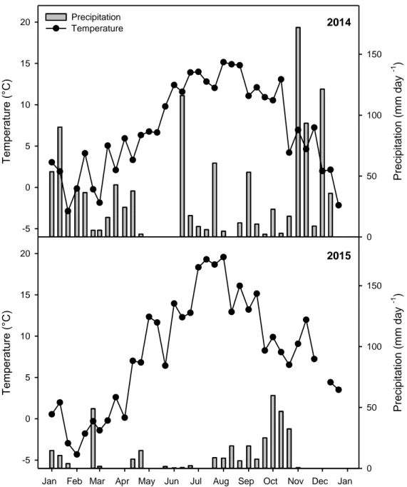
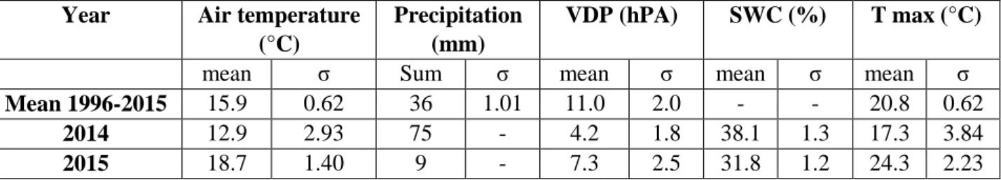
The experiment presented in Chapter 3, was carried out in the Mediterranean beech (Fagus sylvatica L.) forest of Collelongo and is focused on two growing seasons (2014-2015) having different meteorological conditions, with July 2015 characterized by higher monthly temperature and reduced precipitations compared to July 2014. Spectral indices computed at canopy level were used to track changes in CO2 fluxes and in the physiological status. Mainly optical indices related to structure were

found to better track carbon fluxes variation for both 2014 and 2015, thus suggesting that structural parameters are essential drivers at the forest site. Moreover, seasonal patterns of chlorophylls (Chl a and Chl b), carotenoids (b-carotene, lutein, neoxanthin and xanthophyll cycle components) and fluorescence parameters were investigated to evaluate which optical indices better predict changes in photosynthetic pigment levels and energy dissipation mechanisms. Optical indices related to carotenoids composition were indicators of the shifting pigment composition related to stress (July) and senescence (October) during 2015. Thus, spectral indices resulted to be reliable proxies for monitoring carbon fluxes and vegetation dynamics in healthy and stressed vegetation.

Chapter 4 was aimed to validate three fAPAR satellite products, GEOV1, MODIS C5, and MODIS C6, against ground references at the same beech forest in Italy during 2014 and 2015. Three ground reference fAPAR, differing for temporal (continuous or campaign mode) and spatial sampling (single points or Elementary Sampling Units-ESUs), were collected using different devices: 1) Apogee (defined as benchmark in this study); 2) PASTIS; and 3) Digital cameras for collecting hemispherical photographs (DHP). A bottom-up approach for the upscaling process was used. Radiometric values of satellite images were extracted over the ESUs and used to develop empirical transfer functions for upscaling the ground measurements. The resulting high-resolution ground-based maps were aggregated to the spatial resolution of the satellite product to be validated considering the equivalent point spread function of the satellite sensors, and a correlation analysis was performed to accomplish the accuracy assessment. The temporal courses of the three satellite products were found to be consistent with both Apogee and PASTIS, except at the end of the summer season when ground data were more affected by senescent leaves, with both MODIS C5 and C6 displaying larger short-term variability due to their shorter temporal composite period. The three green fAPAR satellite products under study showed good agreement with ground-based maps of canopy fAPAR at 10 h and very low systematic differences.

(7)

1

1.

General introduction

Carbon cycle topic is the common denominator of ecology, oceanography and geochemistry researches due to its central role in the biogeochemical processes. Terrestrial biosphere plays an important role in the global carbon cycle whereas carbon is removed from the atmosphere via photosynthesis by plants [1]. The process by which plants use sunlight to produce organic matter from carbon dioxide through photosynthesis is defined as vegetation productivity [2].Ecosystems carbon dynamics are extremely important in the context of climate change due to their capacity to control the Earth system in a globally significant way [3]. In fact, terrestrial ecosystems can release or absorb relevant greenhouse gases such as carbon dioxide (CO2), methane and nitrous oxide and

control exchanges of energy and water between the atmosphere and the land surface [4]. Considerable amounts of carbon are stored in living vegetation and soil organic matter, and release of this carbon into the atmosphere as CO2 would critically impact the global climate [4]. The biogeochemical carbon

cycle in the ocean and on land will likely continue to respond to climate change and rising atmospheric CO2 concentrations created during the 21st century [5]. Thus, the link between carbon

cycle and global climate change highlights the importance of studying plant ecosystems, not only for their essential role as a carbon sink, but also because climate extremes can potentially impact terrestrial ecosystems causing a shift from a carbon sink towards a carbon source [6].

An area may be a carbon sink if carbon is stored faster than it is being released. Differently, an area is called carbon source if the production of atmospheric carbon from that area exceeds the rate at which carbon is being fixed there. In terrestrial ecosystems, whether an area is a sink or a source depends mostly on the balance between the rate of photosynthesis and the combined rate of respiration and burning [7]. Their role in carbon sequestration varies as the plants have the ability to act as either a carbon sink by removing carbon or as a source by donating carbon to the atmosphere [8]. Ecosystems capacity of acting as carbon sink changes depending on vegetation type. In 2009, the United Nations Environment Programme (UNEP) produced a detailed summary that show the amount of carbon stored (t C/ha) by the different natural ecosystems (Figure 1.1). Ecosystems as tundra and boreal forest are dense in C, which is mainly accumulated in the soil pool, particularly in the permafrost layer for tundra and in soil and litter for boreal forest. The temperate forests, where vegetation growing and decomposition is rapid, have been estimated to store between 150 and 320 tonnes per hectare [9] (Figure 1.1). About the 60% of the carbon stored by this biome is constituted by plant biomass, principally in the form of large woody above-ground organs and deep root systems [9].

(8)

2 Interestingly, Janssens et al. [10] found that European temperate forests are estimated to be taking up 7–12% of European carbon emissions, thus highlighting the potentiality of this kind of ecosystem. Nevertheless, persistent droughts, disturbances such as fire and insect outbreaks, worsened by climate extremes and climate change put the mitigation benefits of the forests at risk [11].

Figure 1.1. Summary of vegetation growth, decomposition, carbon storage and main threats linked to potential C emissions for main natural ecosystems. From Trumper et al. [7].

Differently from the forests, temperate grasslands are moisture and nutrient limited and allocate much of their biomass below ground. Climate change and CO2 may affect grazing systems by altering

species composition; for example, warming will favour tropical (C4) species over temperate (C3) species but CO2 increase would favour C3 grasses [12]. However, despite grasslands have low levels

of plant biomass, their soil organic carbon stocks tend to be higher than those of temperate forests [9]. In ecosystems like desert and dry shrublands, water represent the limiting factor and determines the way in which carbon is processed. While carbon stored is typically lower in the vegetation (2–30 tonnes of carbon per ha), Wohlfahrt et al. [13] suggested that carbon uptake by deserts is much higher than previously thought and that it contributes significantly to the terrestrial carbon sink. Savannas cover large areas of Africa and South America and can store significant amounts of carbon, especially in their soils. The trend and interannual variability of CO2 uptake by terrestrial ecosystems are

dominated by semiarid ecosystems whose carbon balance is strongly associated with circulation-driven variations in both precipitation and temperature [14].Lastly, the largest terrestrial carbon store

(9)

3 is held by tropical forest, where most of the carbon can be found in the vegetation and biomass estimates reaches 170–250 t C per ha [15]. Nepstad et al., [16] informed that predicted changes in temperature, rainfall regimes, and hydrology may promote the dieback of tropical forests. A matching example is the prolonged drought conditions in the Amazon region during 2005 that contributed to a decline in above-ground biomass and triggered a release of 4.40 to 5.87 GtCO2 [17].

Anthropogenic CO2 emissions to the atmosphere were 555 ± 85 PgC (1 PgC = 1015 gC) between

1750 and 2011. Of this amount, fossil fuel combustion and cement production contributed 375 ± 30 PgC and land use change (including deforestation, afforestation and reforestation) contributed 180 ± 80 PgC [5]. Canadell et al. [18] informed that the land sinks of carbon absorb close to one-third of anthropogenic emissions; hence, monitoring terrestrial ecosystems using the latest technical methods is crucial for maintaining the significant potentiality of reducing future emissions of greenhouse gases [19]. Accurate estimates of plant productivity across space and time are thus necessary for quantifying carbon balances at regional to global scales.

Currently, the most renowned methods used for continuous monitoring ecosystem productivity are eddy covariance (EC) technique and remote sensing [20] while ecophysiological techniques have been widely used in the past as non-continuous monitoring of carbon dioxide (CO2). Below, the

methods used in this work for studying plant ecosystems chosen as experimental sites are briefly presented.

1.2 Eddy covariance

Terrestrial gross primary production (GPP) is the entry point of atmospheric CO2 into the

terrestrial ecosystem and it refers to the amount of carbohydrate produced through photosynthesis in a given period of time over a unit area [21]. About half of the carbohydrates are employed by plants for growth and maintenance (autotrophic respiration) [22]. When autotrophic respiration is subtracted from GPP, then the net carbon gain by vegetation (NPP) is obtained [22]. NPP is a key variable for environmental monitoring and is a sensitive indicator of climate change [23]. Besides autotrophic respiration, plants loose carbon through heterotrophic respiration, when heterotrophic organism eat live or dead organic matter and release CO2 to the atmosphere. When also the heterotrophic

respiration is subtracted by NPP, we refer to the net ecosystem productivity (NEP) which has an ecological relevance as it represents the net amount of carbon stored by an ecosystem [22]. NEP can be also expressed as net ecosystem exchange (NEE) which refers to the net CO2 exchange with the

(10)

4 example food, shelter for wildlife, fiber for human society and the aforementioned potentiality for mitigating climate change. For this reason, during the last decades, the need of continuously and accurately track C dynamics became more and more important. In this context, during the last 30 years, the eddy covariance technique emerged as one of the most accurate approaches to measure gas fluxes over large areas. Eddy covariance allows the direct in‐situ measurement of carbon exchange between plant canopy and the atmosphere [25]. The concept behind the method is that the atmosphere contains turbulent motions of upward and downward moving air that transport trace gases (e.g., CO2).

Therefore, the eddy covariance technique samples these turbulent motions to determine the net difference of material moving across the canopy atmosphere interface [24]. Specifically, this technique allows to acquire high frequency (10-20 Hz) measurements of wind speed and direction as well as CO2 and H2O concentrations at a point over the canopy using a three-axis sonic anemometer

and a fast response infrared gas analyzer [26,27]. Flux measurements are typically integrated over periods of half an hour building the basis to calculate carbon and water balances from daily to annual time scales [28].

The widespread use of eddy covariance depended of mainly four reasons: 1) it is a scale appropriate method that assess net CO2 exchange of a whole ecosystem; 2) it provides direct

measurements of net carbon exchange across the canopy-atmosphere interface; 3) it provides measurements having a wide spatial (from hundreds of meters to several kilometers) and temporal scale (continuous measurements from hours to years) [24]. On the other hand, eddy covariance technique is affected by several sources of errors and uncertainties that can be summarized as 1) varying footprints if the ecosystem is inhomogeneous and patchy, 2) instrumentation errors (e.g., acquisition frequency, sensor separation), 3) underestimation of NEE during periods with low turbulence [28].

1.3 Optical sampling: Remote and Proximal Sensing

Optical sampling techniques take advantage of optical properties (reflected or emitted electromagnetic radiation) of a determined surface area using non-contact devices. Three main physical mechanisms may occur when incident radiation interacts with canopy elements: absorption reflection and transmission [29]. For any given material, the amount of solar radiation that is reflected varies with wavelength. When the response (reflectance) characteristics of a certain cover type is plotted against wavelength, this plot is termed the spectral signature of that cover [30]. As most of the diagnostic absorption features of green vegetation are located between 380 and 2500 nm of the

(11)

5 spectrum, the solar reflected radiation in the optical domain is commonly used in vegetation studies (Figure 1.2) [31,32]. Reflectance of vegetation canopies depends on radiative properties of leaves, other non-photosynthetic canopy elements and their spatial organization. Homolová et al. [29] clearly summarize the main characteristic of leaf reflectance spectra as 1) strong and well described absorption of foliar photosynthetic pigments, dominated by chlorophylls, in the visible region (400-700 nm, VIS), 2) leaf structure in the near infrared region ((400-700-1300 nm, NIR), and 3) prevailing water and protein absorptions in the shortwave infrared region (1300-2500 nm, SWIR or middle infrared).

Figure 1.2. Typical spectral signature of leaf and dominant factor controlling leaf reflectance. From Jensen et al. [33].

In particular, in the VIS region, absorption by leaf pigments is the most important process leading to low reflectance values. The main light-absorbing pigments are chlorophyll a and b, carotenoids, xanthophylls and all pigments have overlapping absorption features. Chl a displays maximum absorption in the 410-430 nm (blue) and 600-690 nm regions (red), whereas Chl b shows maximum absorption in the 450-470 nm range (blue). These strong absorption bands induce a reflectance peak in the green domain at about 550 nm. Moreover, carotenoids (Car) absorb most efficiently between 440 and 480 nm (Figure 1.2) [34]. Car absorption waveband overlapping with Chl and lower content of Car than Chl content are the two main obstacles in Car estimation through optical sampling [35].

(12)

6 In the NIR region, the absorption is very low and reflectance reach their maximum values (about 50% in green health leaves), which is largely the result of photon scattering within the leaf tissue at the air-cell interfaces of the mesophyll [36]. The level of reflectance on the NIR domain increases with increasing number of cell layers, cell size and aerial interspaces in the leaf mesophyll. Scattering occurs mainly due to multiple refractions and reflections at the boundary between the hydrated cellular walls and air spaces [37]. In SWIR, leaf optical properties are mainly affected by the water absorption bands that occur at 1450, 1940 and 2700 nm [38]. Among them, the features at 1450 and 1950 nm are the most pronounced. However, strong water vapor absorption in the atmosphere reduces the effectiveness of these spectral information to essentially zero [39]. Protein, cellulose, lignin and starch also influence leaf reflectance in the SWIR [34].

Additionally, both green edge (490-530 nm) and red edge (680-750 nm) regions are widely recognized as two very informative features of the vegetation reflectance [40]. The green edge is a transition region where in situ absorption by Chl a and b and different Car drops sharply from a high value at 480 nm to an almost negligible amount above 531 nm [35]. On the other hand, the red edge region corresponds to the rise of reflectance at the boundary between the chlorophyll absorption feature in the red wavelengths and leaf scattering in the NIR wavelengths [40].

The spectral response of vegetated areas have been widely exploited to develop vegetation indices (VIs). An index is a number qualifying the intensity of a phenomenon which is too complex to be decomposed into known parameters. Accordingly, vegetation indices use a combination of spectral reflectance in different bands for qualitatively and quantitatively evaluating vegetative status using spectral measurements [41]. The advantage of vegetation indices is that they allow obtaining relevant information in a fast and easy way and that the underlying mechanisms are well-understood. [42]. One of the most widely known indices is the Normalized Difference Vegetation Index (NDVI) [43]. It expresses the normalized ratio between the reflected energy in the red chlorophyll absorption region and the reflected energy in the NIR providing an indicator of the ‘greenness’ of the vegetation [44,45]. Likewise, the VIs formulated as combination of red edge bands are frequently employed in plant status assessment. In fact, both the green and red edge regions are important for computation of vegetation indices since they remain sensitive to changes pigment content, reducing the saturation effect and enhancing the sensitivity to moderate-high vegetation densities [46,47].

Balzarolo et al. [48] informed that sensors for optical measurements could be classified into three categories, depending to their spectral bandwidth across the sampled spectrum: (1 broad-band multispectral sensors; (2 narrow-band multispectral sensors; and (3 hyperspectral sensors. Particularly, the broad-band multispectral sensors capture data in a few wavelength channels (bandwidth > 10 nm), the narrow-band multispectral sensors offer fine spectral resolution data (e.g.,

(13)

7 bandwidth ≤ 10 nm) in a few targeted bands instruments, and lastly the hyperspectral sensors measure in very narrow and contiguous (overlapping) channels and can be used to provide more detailed information in the wavelength domain. Consequently, while multispectral system commonly collect data in two to six spectral bands in a single observation, hyperspectral system collect several hundred spectral bands in a single acquisition, thus producing more detailed spectral data [49]. Furthermore, multispectral sensors are characterized by relatively low cost, easy maintenance, and low power consumption, and are hence useful tool for long-term unmanned field measurements. Conversely, hyperspectral devices are more expensive and thus are generally considered less suitable for long-term, automated deployment in the field without additional modifications for unattended use [50]. Both remote sensing (RS) and proximal sensing (PS) are based on the optical properties of vegetation. When we refer to remote and proximal sensing we indicate the practice of obtaining information about an object, area, or phenomenon through the analysis of data acquired by a device that is not in contact with the object, area, or phenomenon under investigation [51].

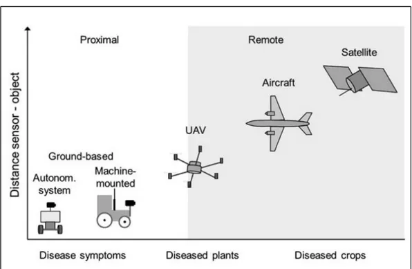
Figure 1.3. Example of proximal and remote sensors and relative distance between sensor and objects of study. From Gullino et al. [52].

The first main difference is that, for RS, the sensor is distant from the object of study by a scale equal to or greater than kilometers while in PS the distance from the sensor to the object of study is on the scale of meters (Figure 1.3) [53]. Moreover, conversely to RS that need geometric and atmosphere corrections, PS can be used without the need of substantial preprocessing of data. Examples of proximal sensors are hand-held, machine mounted or attached to unmanned aerial vehicles (UAVs)

(14)

8 whereas satellites, aircraft or UAVs covering larger areas are typical RS platforms. Lastly, PS has a higher spatial resolution (from 10-3_{to 10}-2_{m) than remote sensing (from 10}-1_{to 10}2_{m) [52].}

1.4 Ecophysiological techniques

Revealing the underlying ecophysiological factors governing net ecosystem exchange (NEE) of CO2 is necessary to strengthen future predictions regarding the role of terrestrial vegetation in the

global C balance and potential climatic change [26].

Among the systems used for measuring the photosynthesis at leaf level, those mainly diffused are gas exchange system and fiber optic fluorimeter measuring chlorophyll fluorescence. Gas exchange system provides direct instantaneous, non-destructive measurements of CO2 concentrations taken up

by photosynthesis and H2O released via transpiration. Particularly, CO2 exchange systems use

enclosure methods, where the leaf is closed in a transparent chamber and the rate of CO2 fixed by the

leaf enclosed is determined by measuring the change in the CO2 concentration of the air flowing

across the chamber [54].

This method involves the use of infrared gas analyzers (IRGAs) that measure the reduction in transmission of infrared wavebands caused by the presence of CO2 between the radiation source and

a detector. Beyond photosynthesis and transpiration, gas exchange systems are able to measure other parameters associated with photosynthesis such as leaf conductance, the intercellular CO2 mole

fraction over a range of conditions that can be manipulated by the researcher [55]. There are mainly two types of gas-exchange systems: closed and open systems. In closed systems, air is continually recycled throughout a system containing a cuvette in which a portion of or a whole plant is placed. Open gas exchange systems have largely replaced the closed systems since when advances in IRGA technology led to the development of commercially available open gas exchange systems. These open systems employ analysis of the gas concentrations in two different chambers: a reference chambers, which has an air stream that is not modified by the presence of a leaf, and a sample chamber, which contains a leaf [56]. Common problems encountered in gas exchange measurements are mainly associated with 1) the fundamentals of the technique, including calibration issue 2) the specific design of the leaf cuvettes used in most commercially available systems and 3) leaf physiology, which are independent of calibration and cuvette designs [55]. However, combining gas-exchange measurements with other techniques allows for an in-depth understanding of numerous processes related to photosynthesis beyond what gas exchange alone can provide.

(15)

9 To maintain energy balance and avoid damage, plants can re-emit excess energy through chlorophyll fluorescence or dissipate it as heat [57]. Chlorophyll fluorescence (Chl F) is one of the most popular techniques in plant physiology because of the easiness with which the user can gain detailed information on the state of photosystem II (PSII) at a relatively low cost. It has had a major role in understanding not just the fundamental mechanisms of photosynthesis but also the responses of plants to environmental change, genetic variation, and ecological diversity [58]. The theory beyond measurements of Chl fluorescence is that the light energy absorbed by chlorophylls associated with PSII can be used to drive photochemistry in which an electron is transferred from the reaction center chlorophyll, P680, to the primary quinone acceptor of PSII, QA. Alternatively, absorbed light energy can be lost from PSII as chlorophyll fluorescence or heat. The processes of photochemistry, chlorophyll fluorescence, and heat loss are in direct competition for excitation energy and these three processes do not exist in isolation but rather in competition with each other [59].

The development of the pulse amplitude-modulated (PAM) technique (an active technique that involves the use of a measuring light and a saturating light pulse) and the subsequent introduction of commercial PAM fluorometers enable the possibility to collect Chl F measurements not just in the laboratory but also in the field [60]. Despite PAM fluorometry has facilitated the study of the acclimation of photosynthesis and helped clarify the link between Chl F and photosynthetic CO2

assimilation, the technique has been restricted to the leaf level for practical reasons, and thus its applicability at the canopy and landscape levels remains unknown. To fill the gap, a new wave of developments attempt to measure Chl F from remote sensing platforms [61]. The remote sensing technique is based on the passive measurement of solar-induced chlorophyll fluorescence (SIF), taking advantage of the fact that atmospheric absorption bands (e.g., the Fraunhofer lines) contain a small fluorescence signal that can be detected with the appropriate narrow-band instruments, allowing quantification of this small signal against a larger background of solar radiation [62,63]. There are intrinsic differences between the basis of active Chl fluorescence measurement methods based on PAM measurement and that of the SIF; thus, consequent challenges are currently encountered [64]. However, the remote measurement of SIF opens a new perspective to assess actual photosynthesis at larger, ecologically relevant scales and provides an alternative approach to study the terrestrial carbon cycle [65].

(16)

10

1.5 State of the art

Traditional sampling techniques for estimating vegetation conditions based on field collection data (e.g. biomass harvesting, pigment analysis), are time-consuming, costly, and not generally applicable to inaccessible regions [30]. From the 1990s to the present, the eddy covariance approach achieved a resounding success in studying ecosystem physiology. This led to the set-up of several network of flux tower such as Euroflux, Ameriflux, MEDEFLUX (the Mediterranean region), AsiaFlux, and OzNet (Australia) thanks to which scientific community improved the understanding of inter- and intra-annual variations in the carbon fluxes at the ecosystem level. However, it is recognized that flux measurements are subject to several sources of error and limitations. Measurements of flux methods require homogenous vegetation in flat terrain around the towers to produce results that are representative of a particular ecosystem, and these conditions are often not perfectly met in natural landscapes [66]. In addition, the footprint of eddy covariance measurements it is affected by variation depending on wind direction and speed, measurement height, and vegetation structure [67]. Furthermore, while number of experimental sites equipped with eddy covariance tower was constantly increasing during the last decades (more than 500 according to Schimel et al. [68], the distribution of the sites was still too limited for quantifying carbon flux at global scale. In this context, satellite-imaging sensors offered synoptic-scale observations of ecosystems conditions and represented invaluable tools to help fill the large spatial gaps of in situ measurements, improving the accuracies of models. Remote sensing complements the restrictive coverage afforded by experimental plots and eddy covariance measurements, facilitating observations of broad-scale patterns of ecosystem functioning [2]. For this reasons, other networks such as SpecNet or Eurospec endorsed the integration of optical sampling with ecosystem-atmosphere fluxes of carbon dioxide [69,70]. Thus, the combination of these methods to address ecosystem-atmosphere fluxes is a relatively new experience and the advent of new tools (principally improved field spectrometers and sampling platforms) have enabled more detailed optical studies of the flux tower footprint [71]. At the moment, the combination of eddy covariance technique and remote sensing provide a promising means to upscale point measurements taken such as carbon fluxes at the ecosystem level to the regional and global scale [72,73].

Recently, the FLuorescence EXplorer (FLEX) mission selected as the European Space Agency (ESA) 8th Earth Explorer (EE8) started to detect the faint red glow of the Sun-Induced Fluorescence signal (SIF) emitted by plants. The FLEX satellite carries the FLuORescence Imaging Spectrometer (FLORIS) to measure fluorescence at the oxygen absorption bands, the reflectance in the red-edge and the Photochemical Reflectance Index (PRI) [74]. Following the work of the afore mentioned

(17)

11 networks (i.e., SpectNet, Eurospec), the current COST Action ES1304 “OPTIMISE” focus on enlarging the ground-truthing spectral networks, standardizing the optical sampling measurements within carbon flux monitoring networks and exploring the measurement and interpretation of multiscale chlorophyll fluorescence data to support satellite fluorescence data. New challenges and future work are mainly linked to present space missions that herald a new range of possibilities for retrieving SIF at the global scale. This could result in improved estimates of the global carbon budget and capacity to track the health of terrestrial ecosystems [61].

1.6 Objectives and thesis structure

The general aim of this research is to take advantage of the combination of different methodologies to better describe vegetation productivity and plant status using mainly 3 approaches: 1) eddy covariance technique, 2) remote and proximal sensing and 3) field sampling. These three approaches represent the common denominator of the study and are shared throughout the different parts of the work. Particularly, the study is organized in 3 parts that are presented after a concise introduction explaining the main characteristics of all the techniques adopted. In Chapter 2, a combination of remote sensing, proximal sensing, eddy covariance, and field sampling are used to monitor the productivity of a typical grassland ecosystem of Northern America. This chapter contribute to the understanding of how optical inputs (both satellite and ground measurements) to a simple empirical Light Use Efficiency model closely track seasonal carbon fluxes and provide a simple proxy to fill gaps in the eddy covariance. Successively, Chapter 3 explores the functionality of a deciduous broadleaf forest in Italy using simultaneously optical sampling, C flux data, leaf eco-physiological and biochemical traits. Spectral indices computed at canopy level were used to track changes in CO2 fluxes and to detect changes in photosynthetic pigment levels and energy dissipation

mechanisms in healthy and stressed vegetation. Besides water, carbon dioxide, and nutrients, plant requires solar radiation in the 400-700 nm range (photosynthetically active radiation or PAR) for photosynthesis. The fraction of PAR absorbed by the vegetation canopy (fAPAR) is therefore an important biophysical variable and is widely used in satellite-based productivity models to estimate gross primary productivity. Chapter 4 presents the validation of three different satellite fAPAR products (PROBA-V GEOV1, MODIS C5 and MODIS C6) against ground references at the same forest site in Italy. Three ground reference fAPAR, differing for temporal and spatial sampling, were collected using different devices (Apogee, PASTIS and DHP) for tracking the seasonal course of fAPAR over the aforementioned deciduous forest, a kind of ecosystem where lack of field data is recognized.

(18)

12 From this overview, it emerges that the three chapter of the thesis are strongly linked by the ecosystem productivity concept. In fact, if on one side, Chapter 2 and Chapter 3 are focused on estimating carbon productivity using optical measurements in different kind of ecosystems, Chapter 4 validates an essential input for photosynthesis modeling. Vegetation productivity is indeed directly related to the interaction of solar radiation with the plant canopy, based on the original logic of Montheith [75], who suggested that productivity was linearly related to vegetation absorbed PAR (light) for photosynthesis.Remotely sensed fAPAR data are widely used as input in carbon productivity models and the fAPAR accuracy is relevant as it has a considerable impact on the fluxes estimated by the model.

(19)

13

2. Monitoring grassland seasonal carbon dynamics, by integrating

optical and eddy covariance measurements

2.1. Introduction

The need to better understand and predict future carbon–climate interactions makes the assessment of biosphere-atmosphere carbon exchange for the various biomes of the planet a critical topic for the scientific community and the policy-makers [76]. There is growing interest in assessing biospheric carbon storage with the hope that management regimes can optimize carbon sequestration. Also, soil processes play important role in global climate change as soils have the potential to act as a net sink for CO2 due to the large amount of carbon currently stored in soil organic matter [77,78].

However, carbon fluxes are inherently dynamic, affected by short-term disturbance and weather events, making evaluation and prediction of carbon storage and climate feedbacks challenging. While much attention has been given to forests for their large feedbacks and carbon sequestration [79], the carbon storage potential of other biomes have been less thoroughly considered, even though many cover large areas, and contribute measurably to overall biospheric carbon uptake and storage.

Rangelands occupy close to 50% of the world’s land area[80],and are defined as lands where indigenous or introduced vegetation is grazed or has the potential to be grazed and are generally considered and managed as natural ecosystems [81]. Rangelands include natural grasslands, savannas, shrublands, deserts, tundra, alpine communities, marshes, and wet meadows [82]. The grassland or prairie biome is particularly important in Canada and in Alberta, as the Grassland Natural Region covers 14.4% of the province [83]. The Dry Mixedgrass Natural Subregion accounts for 47.5% of the Grassland Natural Region area, and thus represents 7% of the area of Alberta province [84]. Grassland provides a number of important services including carbon sequestration and livestock forage. The capacity of grassland ecosystems to sequester carbon is a leading factor in the consideration of policies and practices that maximize carbon storage without compromising managers’ profits [85]. The carbon sequestration of a grassland can vary considerably from year to year since it is influenced both by natural and anthropogenic factors such as temperature, rainfall, species composition, nutrient and water availability, light, grazing pressure and agricultural practices [86,87]. The combination of all these factors makes grasslands considered natural climate change signature ecosystems and so, particularly interesting to be monitored [88–90].

Historically, most attempts to assess ecosystem carbon storage have been based on field sampling of above- and below-ground biomass and carbon, which requires considerable investments in time and personnel [91], and may not capture the temporal dynamics in response to changing conditions.

(20)

14 Ecosystem carbon dynamics have been modeled using different input parameters such as climate [92,93] or soil and nutrient availability [94,95]. However, models often lack spatially or temporally sufficient data inputs, so may not take into account all ecosystem dynamics and interactions.

Significant progress in understanding ecosystem dynamics has been accomplished using the eddy covariance (EC) technique, which quantifies carbon and water vapour fluxes between the biosphere and the atmosphere[96]. This technique has been successfully applied to estimate carbon fluxes in grassland ecosystems [97,98]. Nevertheless, the EC technique is expensive, subject to data gaps, and limited to relatively flat, large landscape regions, so cannot offer universal sampling of fluxes for all locations.

Remote sensing and proximal optical sampling methods can provide cost-effective, uniform samplings under conditions where eddy covariance techniques would be impractical. Satellite remote sensing combined with weather data have been used to model global carbon exchange for many years now, but these current models often disagree with local field measurements due to the coarse scale of their optical and meteorological inputs [99]. For effective carbon policy, fine-grained measurements are needed to match the scale of local land management practices. Recent advances in automation and low-cost optical sensors are making a local-scale optical sensing approach increasingly attractive. Recent studies show that the combined application of remote and proximal optical sensors provide the opportunity to monitor productivity across a wide range of spatial and temporal scales and offer the possibility to relate spectral measurements with carbon fluxes as a foundation for modeling and upscaling [100]. Networks as SpecNet and EUROSPEC have been exploring the possibility of combining flux and spectral measurements[48,69,101]. In this context, models have recently became the bond between remote sensing measurements and carbon fluxes thanks to the increased availability of both information at tower sites. A crucial first step is to evaluate these optical methods in comparison to flux methods to enable proper model parameterization.

The most widely applied model for combining carbon fluxes and optical measurements is the Light Use Efficiency (LUE) model. Originating with the work of Monteith [75,102], more recent parameterizations have been used to estimate gross primary productivity (GPP) based on the equation:

GPP = ε * APARgreen (2.1)

Where APARgreen (absorbed photosynthetically active radiation) represents the amount of

radiation absorbed by green vegetation, and εrepresents the efficiency with which that absorbed light is used by vegetation to fix carbon. To obtain annual GPP, the equation terms can be integrated (summed) [72,99].

(21)

15 APARgreen can be further defined or measured as the product of fAPARgreen (the fraction of photosynthetically active radiation absorbed by green vegetation) and PAR (photosynthetically active radiation, also called the photosynthetic photon flux density, or PPFD):

APARgreen = fAPARgreen x PAR (2.2)

Damm et al. [65] reported that, especially in cropland and grassland, canopy structure and APAR covaries in time during a seasonal cycle. Partitioning between photosynthetic and non-photosynthetic components of vegetation in APAR calculations significantly improve estimation of ecosystem productivity with respect to models driven by total fAPAR [103]. Thus, APARgreen, a measure of

green vegetation structure closely linked to green biomass or leaf area index, plays a dominant role in the model for most grassland ecosystems.

Light use efficiency (ε) relates to vegetation physiology, presumably less important in the case of grasslands and annual systems where canopy growth dominates the seasonal phenological signals detectable with remote sensing [71]. Consequently, most of the variability in grasslands productivity could be explained by changes in APAR [104] when the ecosystem is not stressed [103]. For this reason, the hypothesis of a constant ε over the season (May-October) was adopted in this study.

The strength of the LUE model is related to the possibility of deriving its input values from remote sensing observations [20,99,105]. Several vegetation indices (VIs) have been used to estimate fAPARgreen, most notably the normalized difference vegetation index (NDVI) [106]. When combined

with PAR irradiance, either as a modeled or directly measured value (PAR sensor), fAPAR readily provides a reliable measure of APAR, the primary term in the LUE model (Equation 2.2).

The rising interest in linking carbon flux measurements, proximal (in situ) spectral measurements and remote sensing data has motivated the establishment of a global network of experimental sites in various ecosystems that simultaneously collect optical and flux datasets[69,101]. A key issue in combining optical and flux measurements is the evaluation of temporal scales, as optical and flux measurements vary on different time scales [69]. To our knowledge, few studies explicitly consider the effect on scale of aggregation when comparing optical and flux data, in part because satellite data are typically limited to a single overpass near midday. In this study, we took advantage of the continuous nature of flux and optical data to enable an explicit consideration of temporal aggregation, as recommended by the SpecNet community [101].

The objectives of this study were to:

 assess the seasonal patterns of CO2 exchange, above-ground biomass accumulation, and

optical properties of a prairie grassland ecosystem comparing different optical sampling techniques (NDVI680,800 from field spectrometer measurements, proxy NDVI measurements

(22)

16 from automated sensors on an “optical phenology station,” and MODIS NDVI measurements);

 compare midday data aggregation periods for accurate prediction of fluxes from optical data;  test different NDVI inputs and related biophysical parameters (fAPARgreen and APARgreen)

from both satellite and ground measurements as proxies for flux measurements using the LUE model;

 test the hypothesis of constant ε over the entire season in grassland ecosystem;  demonstrate how optical data can be used for gap-filling eddy covariance datasets.

2.2. Materials and Methods

2.2.1 Study site and experimental design

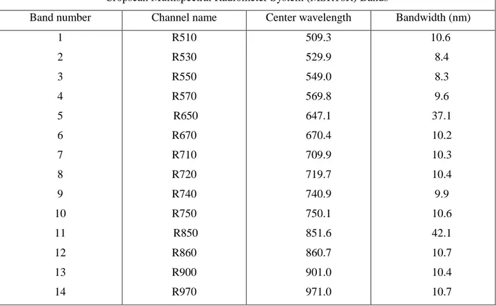
The Mattheis Ranch is a 4977 ha working cattle ranch located near Duchess in southern Alberta, Canada, and is mostly characterized by native prairie vegetation. Recently, this site has become a research area managed by the Rangeland Research Institute (University of Alberta), offering the possibility of long-term monitoring of ecosystem dynamics under management regimes typical of this region. The climate of southern Alberta presents long winters and short, windy summers with extreme temperatures in both seasons, and peak precipitation periods occurring in early summer (June). The rest of the summer usually has lower precipitation, but summer rainfall regimes can vary markedly from year to year, with a similarly variable effect on productivity[87].

Our study site centered around two eddy covariance tower locations designated “E5” (northern site, 50.9056N, 111.8823W) and “E3” (southern site, 50.8671N, 111.9045W), situated about 4.5 km apart. The two sites differed slightly in vegetation cover and microtopography; E5 appeared very flat and uniform, while the E3 landscape varied slightly more than E5 in microtopography and vegetation cover within the presumed flux tower footprint, but was still a relatively uniform grassland-dominated site. The E5 site represents typical dry mixed grass prairie as described by Adams et al. [84]. Based on a clay loam soil, the plant community is dominated by needle-and-thread grass (Hesperostipa comata), Junegrass (Koeleria macrantha), blue grama grass (Bouteloua gracilis), and western wheatgrass (Pascopyrum smithii ). In contrast, the soil at the E3 site is a sandy loam. Dominant grasses include sand grass (Calamovilfa longifolia), needle-and-thread grass (Hesperostipa comata), and low sedge (Carex stenophylla). Slight variations in topography allow forbs such as wild licorice (Glycyrrhiza lepidota) and golden bean (Thermopsis rhombifolia), and shrubs such as wild rose (Rosa woodsii) to flourish [107]. Due to these differences in vegetation, soil type and associated hydrology (not shown), these two sites provided a natural experiment encompassing two contrasting landscapes typical of southern Albertan rangelands.

(23)

17 The measurements at the two grassland sites (E3 and E5), included:

-CO2 flux measurements from eddy covariance,

-continuous, proxy NDVI [101,108] from a set of 2-band radiometers, PAR and PYR (pyranometers), comprising a “phenology station”,

-aboveground biomass samples from a 1 ha area around each flux tower site periodically collected following the sampling scheme reported in Figure 2.1,

- NDVI680, 800 measurements using a field spectrometer collected at regular intervals in the same

area (1 ha) using a 10 m grid spacing (Figure 2.1),

- incident and reflected incoming PAR measurements at each calibration point (numbered circles, Figure 2.1)

- MODIS satellite NDVI data downloaded for the study areas.

Each phenology station was located approximately 10 meters to the southeast of its corresponding flux tower. These two sites were monitored for two consecutive growing seasons (May-September) during 2012 and 2013.

Figure 2.1. Optical and biomass sampling design around each eddy covariance (EC) and phenology station (PS) location. Leaf-level NDVI was sampled at regular intervals within a one hectare region surrounding each flux tower using 10m grid spacing (approx. 100 samples; sampling locations represented by black dots). Biomass sampling and fAPAR calibration occurred at the locations indicated by numbered circles (1-12), with the sampling years indicated by each circle.

(24)

18

2.2.2 NDVI measurements

2.2.2.1 NDVI

680,800

from spectrometer measurements

Narrow-band reflectance measurements were obtained with a dual channel spectrometer (UniSpec-DC, PP-Systems, Amesbury, Massachusetts, USA), which has a spectral range of 305-1130 nm and a ≈3 nm nominal bandwidth (10 nm full width at half maximum). The spectrometer was fitted with two optical fibers, one looking upward and one looking downward, enabling simultaneous sampling of downwelling irradiance and target radiance and correction for variable sky conditions. The upward-looking detector was fitted with a hemispherical cosine head (UNI435, PP Systems, Amesbury MA, USA) and sampled downwelling radiation (about 0.5 m2 per sample); the downward-looking detector was fitted with a fiber optic (UNI684, PP Systems, Amesbury MA, USA) and field-of-view restrictor (hypotube, UNI688, PP Systems, Amesbury MA, USA) and sampled upwelling radiation with a nominal field-of-view of approx. 20 degrees from a distance of approx. 2 m.

The spectrometer sampling procedure involved sampling a 1-hectare grid centered on the flux tower (Figure 2.1). This grid sampling was completed approximately every 20 days during the growing season. Measurements were collected across a 100 X 100 m area (roughly 100 samples on a 10 m grid spacing) within one hour of solar noon. This allowed us to calculate the NDVI of a larger portion of the flux footprint and to compare the field spectral measurements with those derived from the MODIS satellite sensors. In addition to the grid sampling, the field spectrometer was also used to determine NDVI at exactly the same location of each aboveground biomass sampling site for the purpose of NDVI-biomass calibration (numbered circles, Figure 2.1).

Spectral processing software (Multispec, http://specnet.info) was used to calculate raw reflectance values, calculated as the ratio between upwelling surface radiance (Rtarget) and

downwelling solar irradiance (Idownwelling):

Raw reflectance = Rtarget / Idownwelling (2.3)

This software also interpolated reflectance to 1-nm wavebands for index calculation.

The next step was to calculate a cross-calibration value comparing downwelling solar irradiance (Idownwelling) to a 99% reflective white standard panel (Rpanel) (Spectralon, Labsphere Inc., North

Sutton, NH):

(25)

19 This cross-calibration was then used to calculate a corrected reflectance value as follows:

Rcorrected = (Rtarget/Idownwelling) * (Idownwelling/Rpanel) (2.5)

This application of the cross-calibration was corrected for optical differences among sensors and changing irradiance [109]. Both target and panel readings were taken under similar illumination and sun angle conditions. White panel measurements were taken at the beginning and ending of every grid sampling procedure.

Narrowband NDVI was calculated using spectrometer grid data using the 680 nm waveband for the red region of the spectra and the 800 nm waveband for the infrared region using the following formula:

NDVI680,800=(ρ800–ρ680)/(ρ800+ρ680) (2.6)

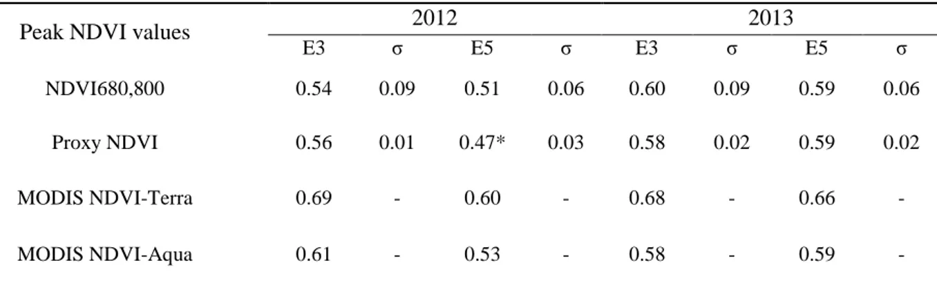
where ρ represents the reflectance at a given waveband, and subscripts indicate the wavelength values used. NDVI680,800 was compared to green biomass and fAPARgreen (see sections 2.2.4 and

2.2.5), but because of the low sampling frequency (about every 20 days) was not compared to daily flux values or used in the LUE model. For these purposes, reflectance spectra from the calibration sites were convolved against PAR, PYR, and MODIS NDVI band responses. These bands were then used to simulate proxy and MODIS NDVI values for calibration against fAPARgreen (see section

2.2.5 below).

2.2.2.2 Proxy NDVI measurements

Each site was monitored with an optical phenology station consisting of a data logger (H21-001, Onset Computer Corporation, Bourne, Massachusetts, USA) and two-band radiometer mounted on a boom and tripod, 3 m above the ground, placed approximately 10 meters southwest of each tower. The sensors detected incoming light (irradiance) and reflected light from the canopy. One band consisted of two PAR (photosynthetic active radiation) sensors (S-LIA, Onset Computer Corporation, Bourne, Massachusetts, USA) that measure the photosynthetic photon flux density (PPFD) within the PAR band (400-700 nm), and the other band consisted of two PYR (pyranometer) sensors (S-LIB, Onset Computer Corporation, Bourne, Massachusetts, USA) measuring across a spectral range from 300 to 1100 nm. Both up- and down-looking sensors had cosine (nominally 180 degree) foreoptics, allowing us to sample a relatively large area (≈ 100 m2_{) immediately adjacent to the flux tower, but}

restricted to a small portion of the total flux footprint (typically > 1 ha, with variations depending on windspeed and wind direction). This phenology station provided a continuous, high temporal resolution proxy NDVI by means of continuous broad-band reflectance in both PAR and PYR bands

(26)

20 sampled every 1-minute during the whole growing season and logged as 15-minute averages, thus monitoring seasonal changes in the vegetation photosynthetic phenology [108]. Additionally, temperature and relative humidity were monitored via appropriate sensors (RH; S-THB-M002, Onset Computer Corporation, Bourne MA, USA) allowing rainy-day optical data to be identified and filtered from the dataset (see Section 2.2.6, below). To derive proxy NDVI values, each sensor pair had been previously cross-calibrated against one another by comparing both upward- and downward-looking sensors in an upward-downward-looking (irradiance) configuration, yielding a coefficient that corrected for any sensor differences (typically less than 5%). These coefficients were then applied to each sensor pair (PAR and PYR) prior to calculating proxy NDVI. Subsequent analyses used the 15-minute averages to calculate midday average APAR and proxy NDVI values for comparison with midday average net CO2 flux from the eddy covariance tower (Figure 2.2).

The phenology station data were used to compute an NDVI proxy [101,108] following the formula:

NDVI proxy = (ρPYR - ρPAR)/(ρPYR + ρPAR) (2.7)

where ρPYR is the reflectance of the solar radiation (PYR band), calculated as the ratio of the

reflected solar radiation to the incoming solar radiation and ρPAR is the reflectance of the

photosynthetically active radiation (PAR band) calculated as the ratio between the reflected PAR and the incoming PAR. This provided a continuous NDVI proxy, which was then averaged over a 5-hour midday period (Figures 2.2-2.3) for comparison with the daily flux measurements. Using the calibrations derived from the harvest sites (equations 2.9-2.11), the NDVI proxy time series was used to derive green fAPAR for the LUE model (Figure 2.2). PAR from the phenology station was then combined with this fAPARgreen to calculate APARgreen in the LUE model (Equation 2.2, Figure 2.2).

(27)

21 Figure 2.2. Experimental design, summarizing steps used in derivation of NDVI and APAR (arrows), and comparisons with net CO2 fluxes (double lines).

2.2.2.3 MODIS NDVI measurements

The NASA Terra and Aqua satellites, which have orbited Earth since 1999 and 2002 respectively, each carry a MODIS (Moderate Resolution Imaging Spectroradiometer) sensor. These satellites pass daily over most of Earth’s surface and provide a nominal 250 m spatial resolution dataset in 36 spectral bands. NDVI values derived from MODIS NDVI products (MOD13Q1 from Terra and MYD13Q1 from Aqua) were downloaded from the Oak Ridge National Laboratory Distributed

Active Archive Center website

(http://daac.ornl.gov/cgi-bin/MODIS/GLBVIZ_1_Glb/modis_subset_order_global_col5.pl). MODIS bands 1 (red, 620 – 670 nm) and 2 (infrared, 841 – 876 nm) were used for MODIS NDVI calculation. The 16-day aggregation period was based on the best observations during the composite period, and the actual collection date for each optimal observation was used to provide more accurate time series. The date-corrected time series was then interpolated to produce a daily MODIS value for comparison with daily flux values (Figure 2.2).

(28)

22

2.2.3 CO

2

flux measurements

Net CO2 fluxes were measured using the eddy covariance (EC) technique [96]. Identical EC flux

towers were deployed at our E3 (50.8672º, -111.9045º) and E5 (50.9057º, -111.8823º) grassland sites. Sites exhibited uniform vegetation cover (described above), providing measureable fluxes from all wind directions (i.e., the flux footprint) except those passing through the tower structures. Each tower was equipped with an open-path infrared gas analyzer (IRGA; LI-7500, LI-COR, Lincoln NE, USA) and a three-dimensional sonic anemometer (CSAT3; Campbell Scientific, Logan UT, USA) to quantify vertical CO2 fluxes. Each EC sensor was affixed at 2.9 m (E3 site) and 3.0 m (E5 site) above

ground level and each IRGA was horizontally separated 15-17 cm from each sonic anemometer. Other sensors to quantify environmental conditions and weather were also fixed to each tower to measure half-hour averages of, for example, air temperature, relative humidity (RH) and soil conditions. All collected data were stored to a datalogger (CR5000, Campbell Scientific).

EC data were analyzed using the software package EddyPro (LI-COR, v. 5.1) to quality check raw data, remove outliers and apply standard corrections to calculate corrected vertical fluxes of CO2.

Raw 10Hz CO2 fluxes were preconditioned by eliminating data spikes greater than 3.5 standard

deviations (σ), temporary drop-outs (10% per bin), and heavily-skewed data (+2>x<-2). Calculated fluxes were corrected for density fluctuations using the Webb et al.[110] procedure. High-pass spectral corrections were implemented after Moncrieff et al. [111], while low-pass spectral corrections, integrating in-situ conditions to determine system cut-off frequencies, were used after Ibrom et al. [112]. Fluxes were further rejected when EC sensors malfunctioned or were affected by moisture, when wind passed through the tower before contacting EC sensors, or when friction velocities fell below 0.1 m s-1 (after Wille et al. [113]). Turbulence tests using the approach of Mauder and Foken [114] were used to remove the poorest-quality fluxes (level 2) when they did occur. Half-hour fluxes below -3σ or above +3σ were considered outliers and removed. Corrections applied to daytime data resulted in the removal of 23.33% of all calculated fluxes across all EC measurements at both sites. For final comparison with optical data (NDVI and APARgreen), a midday average net CO2 flux was calculated based on a 5-hour average, matching the period of averaging used for optical

(29)

23 Figure 2.3. Sample diurnal course of proxy NDVI (from phenology station, circles) and net CO2 flux

(from eddy covariance, triangles), showing average values (open symbols) calculated for the 5-hour midday period (arrow between two vertical lines). Data from site E3, June 7, 2012.

2.2.4 Biomass estimation

From May to August 2012, vegetation samples were harvested from four biomass calibration points approximately every 20 days using a 30 cm diameter ring in both sites (E3 and E5) at a distance of 70 m from the tower in four directions (South-East, North-East, North–West, South-West) (Figure 2.1). The grass material within the ring was cut at ground level and placed into labeled paper bags. The following year, samples from 12 points (4 points above, plus 2 points 17 and 34 m from the tower, in each of four cardinal directions (North, East, South and West) were collected from May to July about every 20 days (Figure 2.1). Biomass samples were collected at each of the harvest sampling points just after the collection of both fAPAR measurements and reflectance measurements, used to calculated narrow-band NDVI (NDVI680,800). Each sample was manually sorted into green biomass

and brown biomass, put into an oven at 60 °C for 24 hours, and weighed. The selection was carried out considering the living tissue that was visibly green as green biomass and the visibly dead tissue as brown biomass. This selection of green and dead biomass allowed us to measure the current year’s production, since the green tissue represented the current year’s growth, and the dead tissue consisted

(30)

24 of the previous year’s growth. For each date, average green and total (green plus brown) above-ground biomass was calculated from the manually sorted and weighed biomass samples. For each sampling date, green biomass was calculated as the average of green biomass at all sampling locations (Figure 2), expressed as g m-2. By providing a direct metric of productivity, this measure of biomass provided an independent check on the validity of the optical (NDVI) measurements and the resulting LUE model.

2.2.5 fAPAR and APAR calibration

At each calibration point (section 2.2.4 above; numbered circles, Figure 2.1), we also measured incident and reflected incoming PAR using a light bar (AccuPAR LP-80, Decagon, Pullman, Washington, USA). Particularly, along on NDVI from spectrometer measurements (Figure 2.1), we measured downwelling PAR above the canopy (S), upwelling PAR reflected from the canopy (R), downwelling PAR below the canopy (T), and upwelling PAR below the canopy (U). Ten measurements were made at each calibration point and averaged, then fAPAR was calculated,

following the procedure described in Accupar user’s manual

(http://www.decagon.com/manuals/LPman12.pdf) and the equation:

fAPAR = 1 – t – r + trs (2.8)

Where t is the fraction of radiation transmitted through the canopy (t = T/S), r is the fraction of radiation reflected by the canopy (r = R/S), and rs is the reflectance of the soil surface (rs = U/T).

These fAPAR measurements were multiplied by the green:total biomass fraction (see section 2.2.4) to calculate a fAPARgreen value (fraction of PAR absorbed by green canopy material) for

comparison with the proxy NDVI values (phenology stations) and NDVI values collected at each harvest site (Figure 2.1). The NDVI- fAPARgreen relationship was later used to derive the APARgreen

term of the LUE model (Equation 2.2), using the following equations derived from the fAPAR calibration sites:

fAPARgreen = (0.8799 * NDVI680,800) – 0.1394 (R2=0.79) (2.9)

fAPARgreen = (1.3916 * NDVIproxy) – 0.3603 (R2=0.82) (2.10)

fAPARgreen = (0.9879 * NDVIMODIS) – 0.2131 (R2=0.79) (2.11)

In accordance with equation 2.2, continuous APARgreen, was calculated as the product of PAR

(31)

25

2.2.6 Filtering and averaging process

Preliminary analysis of the optical data indicated that periods of rainfall led to invalid proxy NDVI values. These periods were easily detectible by evaluating proxy NDVI data relative humidity (RH) values. Proxy NDVI values associated with RH values greater than 76% were filtered from the dataset were discarded to remove invalid data as this threshold best withdraw outliers (data not shown). Similarly, automatic gain control (AGC), an IRGA diagnostic value, identified obstructions blocking the sensor’s optical path. Water droplets, rime, dew, dust or pollen on the optical path impede sensor function and reduce data quality. Proxy NDVI data with associated AGC values greater than 64% were filtered from the dataset. To achieve data comparable to the MODIS values, a midday averaging process was also applied to aggregate proxy NDVI and flux data. To determine how best to integrate flux and optical data, 3 different temporal aggregation periods were considered in our analysis by averaging measurements taken in the time window of 1-hour (13 pm-14 pm), 3-hour (12 am-15 pm) and 5-hour (11 am-16 pm) around midday (approx. 13:30 local daylight savings time). Based on this analysis, a 5 hour averaged value around midday for both CO2 flux and proxy NDVI

was used for our further analyses (Figure 2.2 and Figure 2.3).

2.2.7 Gap filling

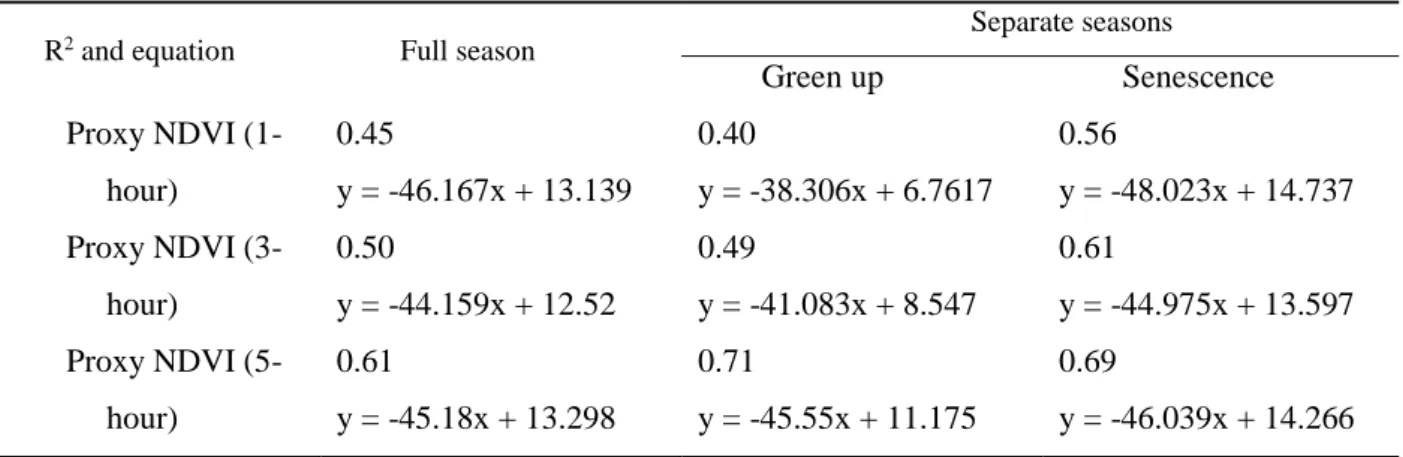
A primary study aim was to test the utility of optical data as a proxy of EC flux measurements, thus allowing gap-filling of the flux dataset. Non-gap-filled flux data were augmented by both filtered proxy NDVI data (which provided the most continuous time-series of all three NDVIs used in this study, but not necessarily the most spatially representative NDVI) and MODIS data (less continuous, but more spatially representative). The relationships between NDVI and fluxes were then used to estimate missing flux data by applying several parameterizations of the LUE model (Equation 2.1), each assuming an invariant efficiency (ε) but variable optical inputs representing APAR. According to LUE model, we used and compared different model terms: parameterizations ranged from simple NDVI (proxy NDVI and MODIS NDVI) to APAR, calculated by combining proxy fAPAR (derived from NDVI) with PAR irradiance (PPFD).

When comparing proxy NDVI to CO2 fluxes, both datasets were averaged for a 5-hour interval

around solar noon (11 am - 4 pm; Figure 2.3) and these values were used as the daily value for flux and proxy NDVI, respectively. These midday average values were then used to model and fill data gaps in the flux data from optical measurements.

When using MODIS NDVI values, NDVI for each day over the entire season was calculated through a linear interpolation of actual date values from MODIS NDVI products (MOD13Q1 from