On the Mean Difference Variance in Random Samples of Student’s Variables

ISSN Online: 2161-7198 ISSN Print: 2161-718X

DOI: 10.4236/ojs.2020.104040 Aug. 10, 2020 659 Open Journal of Statistics

On the Mean Difference Variance in Random

Samples of Student’s Variables

Fabio Manca, Claudia Marin

Department of Education, Psychology, Communication, University of Bari Aldo Moro, Bari, Italy

Abstract

The purpose of this paper is to obtain the expression of the sample mean dif-ference variance of the Student’s distributive model. In the 2007 the study of the mean difference variance, after some decades, was resumed by Campo-basso [1]. Using the Nair’s [2] and Lomnicki’s general results [3], he obtained the variance of sample mean difference for different distributive models (Laplace’s, triangular, power, logit, Pareto’s and Gumbel’s model). In addi-tion he extended the knowledge comparing to the ones already known for the other distributive model (normal, rectangular and exponential model).

Keywords

Mean Difference Variance, Random Sample, Student

1. The Mean Difference Variance General Expression

Let X be a continuous random variable with density function f(x) and distribu-tion funcdistribu-tion F(x). Then, let X X1, 2,,Xn be a simple random sample from

such population; the sample mean difference is

(

)

1 1 1 n n i j i j X X n n = = − ∆ = −

∑∑

(1) The mean value of ∆ is equal to the mean difference of the population

( ) ( )

d d x y f x f y x y

+∞ +∞ −∞ −∞

∆ =

_{∫ ∫}

− (2)

In 1952 Lomnicki [3] obtained the following general expression of the sample mean difference variance

How to cite this paper: Manca, F. and Marin, C. (2020) On the Mean Difference Variance in Random Samples of Student’s Variables. Open Journal of Statistics, 10, 659-663.

https://doi.org/10.4236/ojs.2020.104040 Received: July 9, 2020

Accepted: August 7, 2020 Published: August 10, 2020 Copyright © 2020 by author(s) and Scientific Research Publishing Inc. This work is licensed under the Creative Commons Attribution International License (CC BY 4.0).

http://creativecommons.org/licenses/by/4.0/ Open Access

DOI: 10.4236/ojs.2020.104040 660 Open Journal of Statistics

( )

₍

1

_{) (}

)

2

(

)

(

)

2 var 4 1 16 2 2 2 3 1 n n I n n n  σ  ∆ = _ − + − − − ∆ _ − (3)

in which σ2 _{and Δ are the variance and the mean difference of the considered}

distributive model respectively, whereas

( ) ( ) ( )

d I G x H x f x x +∞ −∞ =

_∫

(4) in which

( )

(

) ( )

d x G x x y f y y −∞ =

_∫

− ₍₅₎ and

( )

( )

H x =G x + −µ x,

(6)

in which µ _{is the mean value of such distributive model.}

The mean value µ and the variance are known for almost all the distributive models. Concerning the mean difference ∆ , the known results are collected in Girone’s and Mazzitelli’s paper [4].

So, to determine the expression of the sample mean difference variance it’s only needed the calculation of I.

2. I Expression for Odd g

The density function of the Student’s distributive model is

( )

(

)

(

)

1 2 2 1 2 , 2 , 2 g x f x x g B g g + + = − ∞ < < +∞ ₍₇₎

in which the parameter g is called number of degrees of freedom.

Using Mathematica software for such model for g=5, 7,,19 the obtained values of Ig are shown in Table 1.

The second term is easily represented by the following formula Table 1. The obtained values of Ig for g=5, 7,,19.

g values di Ig 3 15/(2π2_{) − 1/2} 5 1925/(432π2_{) − 5/18} 7 17,017/(4500π2_{) − 7/30} 9 9,561,123/(2,744,000π2_{) − 3/14} 11 2,369,851/(714,420π2_{) − 11/54} 13 2,170,568,075/(67,6190,592π2_{) − 13/66} 15 3,920,876,125/(1,250,497,248π2_{) − 5/26} 17 1,077,676,328,213/(349,825,132,800π2_{) − 17/90} 19 135,999,445,173,949/(44,757,574,933,500π2_{) − 19/102}

DOI: 10.4236/ojs.2020.104040 661 Open Journal of Statistics

(

)

6 2 g g − − . (8) The first term expression is more complicated to be determined. After several attempts comparing each first term to the previous one, we pointed out the re-curring formula:

(

)(

) (

)(

)

(

) (

)(

)

2 2 4 4 3 3 4 3 8 2 3 7 3 11 g g g g g g g A A g g g − − − − − = − − − , per g=5, 7, (9)

with the initial value

( )

2

3 15 2

A = π .

Considering the previous relation, we came to the following expression of the first Ig term for odd g values greater than 3:

(

)

(

) (

)

(

) (

) (

) (

)

2 2 3 1 2 2 1 3 2 1 3 2 2 2 2 1 6 2 5 6 g g g g g A g g g g Γ_ − _ Γ − Γ + = − Γ Γ − Γ − π, (10)

and then the Ig expression

(

)

(

) (

)

(

) (

) (

) (

)

(

)

2 2 3 1 2 2 1 3 2 1 3 6 2 2 2 2 2 1 6 2 5 6 g g g g g g I g g g g g Γ − Γ − Γ + π    = − − − Γ Γ − Γ − (11)

3. I Expression for Even g

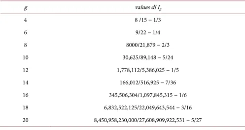
Using again Mathematica software for g=4, 6,, 20 the obtained values of

g

I are shown in Table 2.

The second term of Ig is represented again by the simple formula

(

)

6 2 g g − − . (12) After several attempts, comparing each first term to the previous one, we pointed out the recurring formula:

(

)(

) (

)(

)

(

) (

)(

)

2 2 4 4 3 3 4 3 8 2 3 7 3 11 g g g g g g g A A g g g − − − − − = − − − , per g=6,8, (13)

Table 2. The obtained values of Ig for g=4, 6,, 20.

g values di Ig 4 8 /15 − 1/3 6 9/22 − 1/4 8 8000/21,879 − 2/3 10 30,625/89,148 − 5/24 12 1,778,112/5,386,025 − 1/5 14 166,012/516,925 − 7/36 16 345,506,304/1,097,845,315 − 1/6 18 6,832,522,125/22,049,643,544 − 3/16 20 8,450,958,230,000/27,608,909,922,531 − 5/27

DOI: 10.4236/ojs.2020.104040 662 Open Journal of Statistics with the initial value A4 =8 15. It has to be noticed that the recurring formula

is the same one as the odd case.

Considering the previous relation, we came to the following expression of the first Ig term for even g values greater than 4:

(

) (

) (

) (

)

(

) (

) (

)

2 3 2 4 2 3 2 2 2 1 3 2 1 3 2 2 1 6 2 5 6 g g g g g g g A g g g − _{− Γ − Γ − Γ +} = Γ Γ − Γ − (14)

and then the Ig expression

(

) (

) (

) (

)

(

) (

) (

)

(

)

2 3 2 4 2 3 2 2 2 1 3 2 1 3 6 2 2 2 1 6 2 5 6 g g g g g g g g I g g g g − _{− Γ − Γ − Γ +} = − − Γ Γ − Γ − (15)

Through some algebraic steps it is easily verified that the two Ig formulas

for the odd case and the even one are the same and, moreover, a single more compact expression is the following

(

) (

)

(

) (

) (

) (

) (

)

(

)

3 2 2 2 3 2 1 3 2 1 3 6 2 1 2 2 , 2 2 1 6 2 5 6 g g g g g g I g g g B g g g g − _{Γ − Γ +} = − − − − Γ − Γ − (16)

4. The Sample Mean Difference Variance

Let us remind that for the Student’s distributive model the expressions of the mean value (µ), the variance (σ2) and the mean difference (Δ) are the

follow-ing: 0

µ

= _{, (17)} 2 2 g g σ = − ,

(18)

(

) (

)

(

) (

) (

)

2 3 1 2 , 1 2 2 1 , 2 , 2 2g g B g g g B g g B g g − − +     ∆ = − . (19)

Using the Lomnicki’s formula we came to the following expression of the mean difference variance for the Student’s distributive model:

( )

₍

(

_{) (}

)

₎

[

_{[ ]}

]

(

)

(

)

(

)

(

)

( )(

)

(

)

[ ]

(

)

2 2 5 2 6 2 2 2 1 2 1 2 var 2 3 2 4 1 3 2 1 ₁ 8 3 1 2 2 2 2 1 g_{g g g n} g n g n n _{n n} g g h g n g n n g g − _{Γ − Γ −  −} + _{ } + − − Γ − Γ_ − _ − + π − Γ = − ∆ (20) in which

( )

₍

(

2 1 3

_{) (}

) (

2 1 3

)

₎

2 1 6 2 5 6 g g h g g g Γ − Γ + = Γ − Γ − (21)

It is easily checked that, as g diverges,

( )

72 48 3 4

₍

(

48 24 3

₎

4

)

var 3 1 n n n − + − + + π π ∆ = − π , (22)

DOI: 10.4236/ojs.2020.104040 663 Open Journal of Statistics that represents the sample difference variance for the normal model. It is also easily verified that, as n diverges, the above mentioned variance approaches zero, which means that ∆ is also a consistent estimator.

5. Conclusions

The sample mean difference ∆ is a correct estimator of the mean difference population for every distributive model. To verify if it is also consistent or not we need to calculate its variance, in this paper we have obtained the variance of ∆ _{formal expression for the Student’s distributive model in terms of the} pa-rameter g (degrees of freedom) and of the sample size n.

Because, even for the Student’s distributive model, such variance approaches zero as the sample size n diverges, ∆ results consistent. As g diverges the Stu-dent’s distributive model tends to the normal one. As a matter of fact the vari-ance of ∆ expression we found approaches the varivari-ance of ∆ for the normal distributive model.

Acknowledgements

The helpful and constructive comments of a referee which lead to an improve-ment of the presentation of the paper and support from the editorial staff of Open Journal of Statistics to process the paper are all gratefully acknowledged.

Conflicts of Interest

The authors declare no conflicts of interest regarding the publication of this pa-per.

References

[1] Campobasso, F. (2007) Alcuni risultati sulla varianza della differenza media camp- ionaria. Annals of the Department of Statistical Sciences, 6.

[2] Nair, U.S. (1936) The Standard Error of Gini’s Mean Difference. Biometrika, 28, 428-436. https://doi.org/10.2307/2333957

[3] Lomnicki, Z.A. (1952) The Standard Error of Gini’s Mean Difference. Annals of Mathematical Statistics, 23, 635-637. https://doi.org/10.1214/aoms/1177729346 [4] Girone, G. and Mazzitelli, D. (2007) La differenza media nei principali modelli