SEISMIC PERFORMANCE OF STEEL DUAL SYSTEMS WITH BRBS
AND MOMENT-RESISTING FRAMES
Enrico TUBALDI1, Fabio FREDDI2, Alessandro ZONA3, Andrea DALL’ASTA4
ABSTRACT
Buckling-restrained braces (BRBs) are energy dissipation devices which have proven to be very effective in improving the performance of existing and new building frames. However, their post-elastic stiffness may lead to excessive residual deformations in the systems to be protected, and this may cause irreparable damage and jeopardize the capability of withstanding multiple shocks. Previous studies demonstrated that buckling-restrained braced frames (BRBFs) can be used in conjunction with special moment-resisting frames to form a dual system, able to minimize the residual drifts and optimize the performances of the BRBFs. The objective of this present paper is to provide recommendations regarding the proportioning in terms of forces, stiffness and ductility of the two systems. For this purpose, an extensive parametric analysis under the single degree of freedom approximation for the dual system is carried out to shed light on the parameters that control the seismic performance and residual capacity of frames equipped with BRBs. A non-dimensional formulation of the problem allows investigating wide ranges of configurations, including the case of BRBFs and the case of BRBFs forming a dual system with moment-resisting frames. The results of this study provide useful information for the preliminary sizing and the optimal choice of the design parameters of structural systems equipped with BRBs.
Keywords: Buckling-Restrained Braces; Dual Systems; Cumulative Ductility; Residual Displacement; Seismic Performance
1. INTRODUCTION
Buckling-restrained braces (BRBs) are elastoplastic passive energy dissipation devices (e.g. Soong and Spencer 2002, Christopoulos and Filiatrault 2006) employed in buckling-restrained braced frames (BRBFs) to resist the horizontal seismic-induced forces and dissipate the seismic energy. The use of these devices is gaining popularity for both new constructions and rehabilitation of existing buildings. In BRBs, a sleeve provides buckling resistance to an unbonded core that resists axial stress. As buckling is prevented, the core of the BRB can develop axial yielding in compression in addition to that in tension, ensuring an almost symmetric hysteretic behaviour.
While the large and stable dissipation capacity of BRBs is corroborated by many experimental studies (e.g. Black et al. 2002, Merritt el al. 2003), their low post-yield stiffness may result in inter-story drift concentration, (Zona et al. 2012), and large residual inter-storey drifts. The latter problem is associated with high repair costs and disruption of the building use or occupation (Erochko et al. 2010). Sabelli et
al. (2003) studied the seismic performance of buckling-restrained braced frames (BRBFs) reporting residual drifts on average in the range of 40 to 60% of the maximum drift. Usually, residual drifts lower than 0.5% are deemed acceptable for building frames since they would allow building reparability, e.g. doors, windows and elevators would still be functional (Iwata et al. 2006, McCormick et al. 2008). However, BRBFs designed according to the codes may exhibit residual drifts higher than this limit even under the design basis earthquake. In addition, the performance under
1Lecturer, Dept. of Civil & Environmental Eng., Strathclyde Univ., Glasgow, UK, [email protected] 2Lecturer, Dept. Civil, Environment & Geomatic Eng., Univ. College of London, UK, [email protected] 3Associate Professor, School Arch. & Design, Camerino Univ., Ascoli Piceno, Italy, [email protected] 4Professor, School Arch. & Design, Camerino Univ., Ascoli Piceno, Italy, [email protected]
2
aftershocks may also be jeopardized by excessive residual drifts due to the main shock.
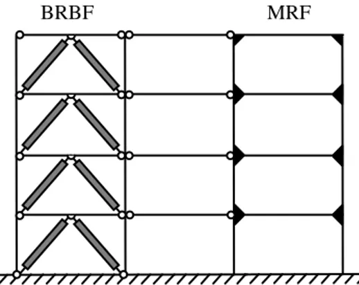
This issue, which may impair the cost-effectiveness of BRBFs, could be avoided by using a special steel moment-resisting frame (MRF) in parallel with the BRBF to create a dual system configuration (Kiggins and Uang 2006, Ariyaratana and Fahnestock 2011, Baiguera et al. 2016). The ASCE/SEI 7-10 (207-10) considers the situation of a dual system that combines a stiff primary seismic force-resisting system (e.g. BRBFs) with a special MRFs, as schematically represented in Figure 1. According to ASCE/SEI 7-10 (2010), the MRF in dual systems should be capable of resisting at least 25% of the prescribed seismic force. Kiggins and Uang 2006 investigated the seismic response of a 3-storey and a 6-storey BRBFs with and without a parallel MRFs designed to resist the 25% of the design base shear, showing that the MRF in parallel allows to reduce the residual drifts by about 50%, while providing similar performances in terms of peak inter-story drift demand. The efficiency of dual BRBF-MRF systems is also demonstrated in Ariyaratana and Fahnestock (2011) while using as case study a 7-storey frame. BRBs are also employed to enhance the lateral strength, stiffness as well as the dissipation capacity of existing reinforced concrete (RC) buildings (Freddi et al. 2013, Di Sarno and Manfredi 2010). RC frames and BRBFs also form a dual system, with the former often contributing to more the 25% of the total base shear.
MRF BRBF
Figure 1. Schematic dual system combining a buckling-restrained braced frame (BRBF) and a special moment resisting frame (MRF)
The works above evaluated the efficiency of BRBFs used to form dual systems by considering only few case studies, without providing general indications regarding the influence of the shear ratio, stiffness ratio and target design ductility of the two systems on the seismic performance and their optimal values. In this work, an extensive parametric investigation is carried out to shed light on this behavioural aspect, and provide useful recommendations for preliminary design. The problem is analysed by assuming that both the BRBF and the MRF can be described as single degree of freedom (SDOF) systems. This representation, demonstrated suitable for low-rise frames under some regularity conditions (e.g. Kim and Seo 2004, Choi and Kim 2006, Ragni et al. 2011, Maley et al. 2010), allows to derive a non-dimensional formulation of the problem and highlight the few characteristic parameters that control the seismic performance. By changing the values of these parameters, it is possible to explore the performance of wide ranges of configurations under a set of ground motion records representative of the uncertainty of the seismic input.
Engineering demand parameters (EDPs) of interest include the peak normalized response, the normalized residual displacements, and the cumulative ductility demand in the BRBs. These EDPs are evaluated in correspondence of the design condition, where the BRBF and MRF attain simultaneously their target ductility capacity. It is noteworthy that some response parameters such as the residual displacements may exhibit larger dispersion due to record-to-record variability effects compared to others (Ruiz Garcia and Miranda 2006). Thus, the reported parametric study results include not only the median (estimated by the geometric mean GM), but also the lognormal standard deviation of the EDPs of interest. In order to provide recommendations useful for the optimal design of the coupled system, different design choices are investigated, corresponding to various combinations of the ductility demand of the BRBF and MRF, within the respective capacity limit.
3
2. PROBLEM FORMULATION
2.1 Equation of motion
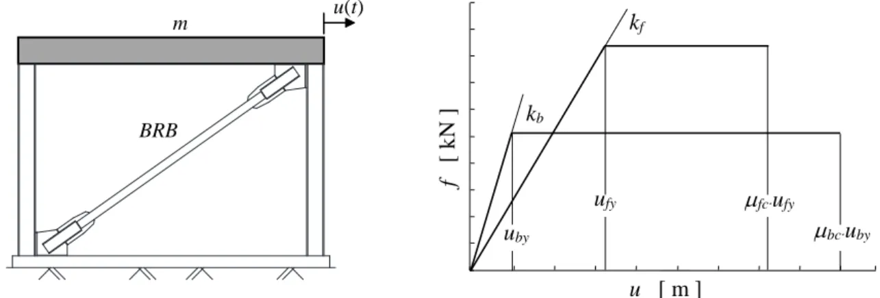
The equation of motion governing the seismic response of a SDOF system representative of a dual system, as represented in Figure 2(a) can be expressed as:
f
f b g
mu t
c u t
f
f
u
t
(1)where m and cf denote respectively the mass and the viscous damping constant of the system, ff the
resisting force of the frame, fb the resisting force of the BRBF, üg(t) the ground acceleration input.
u(t) m BRB u [ m ] f [ kN ] ufy fcufy bcuby uby kb kf
Figure 2. a) SDOF dual system with BRB, b) Constitutive law of the dual systems.
The frame is assumed to have elastoplastic behaviour, with initial stiffness kf, yield displacement ufy
and ductility capacity fc as reported in Figure 2(b). The BRBF system has a constitutive law described
by the model of Zona and Dall’Asta (2012). This model is characterized by a number of parameters describing the hardening and the hysteretic behaviour. In order to keep the problem as simple as possible, most of them are assumed as fixed and the BRBF hysteretic behaviour is controlled only by the initial stiffness kb, the yield displacement uby and ductility capacity bc. These parameters are the
ones which exhibit significant variation from device to device and they are the design parameters explicitly reported in catalogues. The two models working in parallel, whose constitutive behaviour is illustrated in Figure 2(b), are representative of the dual SDOF system.
Such a model can describe a wide range of structural configurations, e.g. the case of BRBFs combined with MRFs to form a dual system (Kiggins and Uang 2006, Ariyaratana and Fahnestock 2011, Baiguera et al. 2016) or retrofit applications involving BRBs inserted into existing RC frames (Freddi
et al. 2013, Di Sarno and Manfredi 2010).
The seismic input is characterized by significant uncertainty affecting not only its intensity, but also the duration and frequency content. As usual in Performance Based Earthquake Engineering, the uncertainty of the seismic input is treated by introducing a seismic intensity measure (IM) (Shome et
al. 1998, Freddi et al. 2017) whose statistical description is the object of the hazard analysis. The
ground motion randomness for a fixed intensity level im, usually denoted as record-to-record variability, can be described by selecting a set of ground motion realizations characterized by a different duration and frequency content and scaling these records to the common im value. The system response for a ground motion with an intensity im can be expressed as:
f
f b g
mu t
c u t
f
f
im u
t
(2)where ug
t denotes the ground motion records scaled such that im = 1 for that record.4
and hazard computability (Shome et al. 1998, Freddi et al. 2017, Tubaldi et al. 2015, Galasso et al. 2015). In this paper, the spectral acceleration Sa(0,), at the fundamental circular frequency of the system, 0, and for the damping factor is employed as IM.
2.2 Non-dimensional formulation
Based on Equation 2, the maximum relative displacement of the system, umax, under the fixed ground motion with history ug
t , can be expressed as:
max
,
f,
f, u ,
fy b, u ,
byu
f m c k
k
im
(3)The 8 variables appearing in Equation 3 have dimensions: [umax]=L, [m]=M, [cf]=MT-1, [kf]=ML-2,
[ufy]=L, [kb]=ML-2, [uby]=L, [im]=LT-2 where the 3 physical dimensions are the time T, the mass M, and
the length L. By applying the Buckingam -theorem (Barenblatt 1987), Equation 3 can be conveniently reformulated in terms of dimensionless parameters, denoted as -terms identifying the parameters that control the seismic response of the system and also reducing the number of variables. The problem involves 3 physical dimensions and 8 dimensional variables, thus, only 8 - 3 = 5 dimensionless parameters are needed. By selecting the systems mass m, the seismic intensity measure
im, and the initial frame stiffness kf as repeating variables, the -terms can be derived and after
manipulation, the following alternative set of -terms can be obtained, which are given below a physical interpretation:
2
max 0 max max
0 , , , , 2 f b f b fy by f c u u u f im u u m f
(4)where 02 = (kb + kf)/m denotes the square of the circular frequency of the SDOF dual system.
The parameter denotes the displacement demand umax normalized with respect to the displacement value im
02. By considering Sa
0,
as IM, it can be interpreted to as the displacement amplification factor, being the ratio between umax and the pseudo-spectral displacement
20, 0, 0
d a
S
S
. The parameters f and b denote the ductility demand respectively of theMRF and the BRBF. The parameter , representing the ratio between the strength capacity of the bracing system and that of the frame, was already employed in Freddi et al. (2013) for evaluating the retrofit effectiveness of BRBFs inserted within a reinforced concrete frame. The strength ratio considered in SEI/ASCE 7-10 (2010) to define a dual system is equal to:
1 1 f b f V V V
(5)
Thus, should be lower than d = 3 for the system to be considered as dual.
It is important to observe that while the parameters f, b and of Equation 4 depend on the response
of the system through umax, the parameters and are independent from the response.
Other EDPs of interest for the performance assessment can be derived from the non-dimensional solution. In particular, the following EDPs are considered:
, , bp cum b cum by u u
, 2 0 , res res elu
im
, max res res u u
, max abs a im
(6)where b,cum denotes the normalized cumulative plasticity (i.e., ductility) demand of the BRBF, res,el
5
ratio between the residual and the peak inelastic displacement of the system, and abs the absolute
acceleration amax normalized by the seismic intensity im.
The system response in terms of these EDPs depends on the characteristics of the input via the circular frequency 0. In fact, seismic inputs with the same intensity im but with different characteristics propagate differently and have different effects on systems with different natural frequencies 0. This has been demonstrated in Tubaldi et al. (2015) by considering SDOF systems with nonlinear viscous dampers but the same reasoning holds for the problem considered in this study. Alternatively, the ratio 0/g between the bare system frequency and a frequency synthetically representing the ground motion frequency content could be considered (Dimitrakopoulos et al. 2009, Karavasilis et al. 2011 and Málaga-Chuquitaype 2015).
3. PERFORMANCE ASSESSMENT METHODOLOGY
The objective of the proposed study is to evaluate how the coupled system behaves in correspondence of the design condition, defined by the target ductility levels of the BRBF and the MRF (Freddi et al. 2013, Zona et al. 2012), respectively bt and ft, corresponding to the design earthquake input. More
specifically, assuming a target ductility level bt≤ bc for the BRBF and a target ductility level ft ≤ fc
for the frame, the design condition corresponds to b =bt and f =ft under the assumed seismic input.
For example, the BRBF may be designed to attain a ductility demand bt = 10, while the MRF may be
designed to remain elastic with ft =1. In design practice, this condition is ensured by considering a
deterministic performance (Dall’Asta et al. 2016), i.e., by considering the mean ductility demand obtained for the different earthquake inputs describing the record-to-record variability effects.
The above design criterion imposes a constraint on the values that can be assumed by the non-dimensional problem parameters, which makes the methodology different from those followed in other researches on similar systems employing non-dimensionalization and considering free parameters variations (Tubaldi et al. 2015, Karavasilis et al. 2011, Málaga-Chuquitaype 2015). Given the system properties independent from the response ,, ft, bt, , the design condition can be
found by the following optimization problem: find the value * of the normalized displacement
demand such as f fc and b bc, where the over score denotes the mean across the samples, and thus
denotes the mean ductility demand. The following procedure can be applied to ensure the attainment of the design condition under the set of records employed to describe the seismic input:1. Assign arbitrary values to the target mean displacement demand umax* and to m, e.g. * max
u = 1 m and m = 1ton. The corresponding non-dimensional parameter values are: cf = 2m0,
* max/
fy f
u u , ubyumax* /b, kf 02m
1ufy/uby
, kb
ufy/uby
kf; 2. Scale the records to a common value of the intensity measure e.g. im = 1; 3. Perform nonlinear dynamic analyses for the different records;4. Evaluate the mean system displacement response
u
max. Ifu
max is equal to the target value *max
u , then
*, where
* umax*
02 im, and go to step 5. Otherwise multiply im by the ratio umax* /umaxand restart step 2. This procedure corresponds to a linear interpolation between the relationu
max and im. If this procedure does not converge, resort can be made to any optimization algorithm;5. Evaluate the statistics of res,res,el,abs,and b,cum.
Steps 1-4 ensure that the design condition of the MRF and the BRBFs attaining simultaneously their performance target under the design earthquake input is achieved.
6
4. PARAMETRIC STUDY
4.1 System properties
The performance of the systems corresponding to different values of 0, , ft, bt, is studied in this
section considering the constraint posed by the attainment of the design condition, which corresponds to =*. The parameter
0 is varied in a range corresponding to a vibration period T0 = 2/0 in the
range between 0 and 4 sec. The strength ratio assumes the values in the range between 0 and 100. The lower bound = 0 represents the case of the bare frame, whereas the upper bound represents the case of frame with pinned connections where the horizontal stiffness and resistance is provided only by the BRBF. The parameter ft assumes values in the range between 1 and 4. The case ft = 1
corresponds to a design condition where the frame behaves in its elastic range under the design earthquake. The case ft = 4 corresponds to a highly ductile behaviour of the frame under the design
earthquake. The parameter bt assumes values in the range between 5 and 20. Values of 15-20 are
typical ones for the ductility capacity of a BRB device. In some situations, such as the seismic retrofit of RC frames (Freddi et al. 2013), the BRB device is arranged in series with an elastic brace exhibiting adequate over-strength. This leads to reduced values of the ductility capacity which may attain the lower bound of 5 for a very flexible elastic brace (Ragni et al. 2011). The value of 2% is assumed for the damping factor in this study.
4.2 Seismic input description
A set of 28 ground motions is considered in the parametric study to describe the record-to-record variability (Tubaldi et al. 2015). The records have been selected from the PEER strong motion database (FEMA P695) on the basis of three fundamental parameters: site class, source distance, and magnitude. Ground motions associated with site class B, as defined in Eurocode 8, source-to-site distance, R, greater than 10km, and a moment magnitude, Mw, in the range between 6.0 and 7.5 are considered. The record number is deemed sufficient to obtain accurate response estimates, given the efficiency of the intensity measure employed (Shome et al. 1998).
4.3 Parametric study results
Figure 3 shows the GM of the normalized peak displacement demand vs the base shear ratio , for different values of the target BRBF ductility bt. The different figures refer to different values of T0 and of the target frame ductility ft. All the curves attain the same value for = 0 (MRF only), and in
particular for ft = 1 they attain a value of about 1. This result is expected, since for = 0 the response
is not dependent on the BRBF’s ductility capacity, and for ft = 1 the system behaves (on average)
elastically, so that the inelastic displacement coincides with the elastic one. On the other hand, for = 0 and ft = 4, a simple bilinear oscillator is obtained and can be significantly different than 1. In
particular, higher values of the normalized peak displacement are observed for low values of the period T0. In the case of dual system ( > 0), for low periods and increasing values of , the normalized peak displacement increases, whereas for high periods remains almost constant and slightly less than 1.
Figure 4 illustrates the variation of the normalized displacement response dispersion. The lowest dispersion values are observed for = 0. For low periods, the dispersion increases for increasing values of , of bt, and of ft, and can attain very high values of the order of 1 in the case of pure
BRBF. For the other, higher periods considered, it is practically constant and equal to about 0.5. These trends also reflect the reduction of efficiency of the IM considered in this study, yielding an almost null dispersion only in the case of = 0 and ft = 1, i.e., of the elastic bare frame. It is noteworthy that
the dispersion is not exactly 0 even for this case, because only the mean ductility demand is equal to 1, and thus for some records the system behaves inelastically.
7 10-1 100 101 102 [ - ] 0 2 4 6 8 T0 = 0.1sec GM (=0) ) = 1.0376 10-1 100 101 102 [ - ] 0 GM (=0)) = 0.9994 0.5 1 1.5 10-1 100 101 102 [ - ] 0 GM (=0)) = 0.9999 0.5 1 1.5
a)
c)
e)
10-1 100 101 102 [ - ] 0 2 4 6 8 GM (=0)) = 2.3322 10-1 100 101 102 [ - ] 0 GM(=0)) = 0.9019 0.5 1 1.5 10-1 100 101 102 [ - ] 0 GM (=0)) = 0.8329 0.5 1 1.5b)
d)
f)
ft = 1 T0 = 1sec ft = 1 T0 = 4sec ft = 1 T0 = 0.1sec ft = 4 T0 = 1sec ft = 4 ft = 4 T0 = 4sec 5 10 15 20 GM ) [ - ] ] GM ) [ - ] ] GM ) [ - ] ] GM ) [ - ] ] GM ) [ - ] ] GM ) [ - ] ]Figure 3. Geometric mean of the normalized peak displacement demand vs the base shear ratio , for different values of T0 (0.1, 1 and 4 sec), of ft (1 and 4) and of bt (5, 10, 15 and 20)
10-1 100 101 102 [ - ] 0 T0 = 0.1sec (=0)) = 0.13418 10-1 100 101 102 [ - ] 0 (=0)) = 0.001664 10- 100 101 102 [ - ] 0 (=0)) = 0.0002223 0.5 1
a)
c)
e)
10-1 100 101 102 [ - ] 0 (=0)) = 0.67169 10-1 100 101 102 [ - ] 0 (=0)) = 0.46868 10- 100 101 102 [ - ] 0 (=0)) = 0.37954b)
d)
f)
ft = 1 T0 = 1sec ft = 1 T0 = 4sec ft = 1 T0 = 0.1sec ft = 4 T0 = 1sec ft = 4 ft = 4 T0 = 4sec 5 10 15 20 ) [ - ] ] ) [ - ] ] ) [ - ] ] ) [ - ] ] ) [ - ] ] ) [ - ] ] 0.5 1 0.5 1 0.5 1 0.5 1 0.5 1Figure 4. Dispersion of the normalized peak displacement demand vs the base shear ratio , for different values of T0 (0.1, 1 and 4 sec), of ft (1 and 4) and of bt (5, 10, 15 and 20)
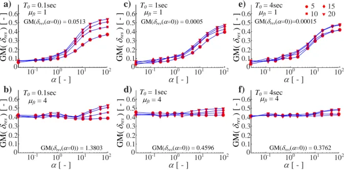
Figure 5 shows the GM of the normalized residual displacement demand res vs the base shear ratio ,
for different values of the target BRBF ductility bt. The different figures refer to different values of T0 and of the target frame ductility ft. In general, the period T0 does not influence significantly this response parameter. Moreover, when the system behaves linearly ( = 0,ft = 1), the residual
displacements are zero. Obviously, adding in parallel to a linear system a nonlinear one ( > 0 in Figure 5 (a, c, e)) results in an increase of residual displacements. This increase is higher for higher values of the target BRBF ductility bt. Thus, high values of must be avoided to limit residual
displacements. The limit d = 3 posed by SEI/ASCE 7-10 (2010) on the maximum values of in dual
systems provides a good control of the residual displacements, ensuring values of res lower than 0.25.
On the other hand, if the frame exhibits a nonlinear behaviour with a target ductility ft = 4, then it is
8
BRBs ( > 0 in Figure 5 (b, d, f)) does not increase them significantly. It is noteworthy that the values of res for = 0 and ft = 4 are similar to the ones observed in Liossatou and Fardis (2015) for an
elasto-plastic system with a strength reduction factor of 4 under a different set of records than the one considered in this study.
10-1 100 101 102 [ - ] 0 T0 = 0.1sec GM(res(=0)) = 0.0513 10-1 100 101 102 [ - ] 0 10-1 100 101 102 [ - ] 0
a)
c)
e)
10-1 100 101 102 [ - ] 0 10-1 100 101 102 [ - ] 0 10-1 100 101 102 [ - ] 0b)
d)
f)
ft = 1 T0 = 1sec ft = 1 T0 = 4sec ft = 1 ft = 4 T0 = 1sec ft = 4 ft = 4 T0 = 4sec 5 10 15 20 0.2 0.4 0.6 0.5 0.3 0.1 0.2 0.4 0.6 0.5 0.3 0.1 0.2 0.4 0.6 0.5 0.3 0.1 0.2 0.4 0.6 0.5 0.3 0.1 0.2 0.4 0.6 0.5 0.3 0.1 0.2 0.4 0.6 0.5 0.3 0.1 T0 = 0.1sec G M ( res ) [ ] G M ( res ) [ ] G M ( res ) [ ] GM(res(=0)) = 1.3803 GM(res(=0)) = 0.4596 GM(res(=0)) = 0.0005 GM(res(=0))=0.00015 GM(res(=0)) = 0.3762 G M ( res ) [ ] G M ( res ) [ ] G M ( res ) [ ]Figure 5. Geometric mean of the normalized residual displacement demand res vs the base shear ratio , for different values of T0 (0.1, 1 and 4 sec), of ft (1 and 4) and of bt (5, 10, 15 and 20)
Figure 6 shows the values of the dispersion of res. These values are very high, particularly for low
values of the frame ductility capacity and low values of However, it should be noted that the dispersion is similar to the coefficient of variation (c.o.v.) only for low values of . In fact, the values assumed by the c.o.v. for res are never higher than 1.5.
10-1 100 101 102 [ - ] 0 T0 = 0.1sec res(=0)) = 16.42 10-1 100 101 102 [ - ] 0 res(=0)) = 12.86 10-1 100 101 102 [ - ] 0 res(=0)) = 1.0401
a)
c)
e)
10-1 100 101 102 [ - ] 0 res(=0)) = 1.3212 10-1 100 101 102 [ - ] 0 res(=0)) = 1.0169 10-1 100 101 102 [ - ] 0 res(=0)) = 1.4399b)
d)
f)
ft = 1 T0 = 1sec ft = 1 T0 = 4sec ft = 1 T0 = 0.1sec ft = 4 T0 = 1sec ft = 4 ft = 4 T0 = 4sec 5 10 15 20 res ) [ - ] ] res ) [ - ] ] res ) [ - ] ] res ) [ - ] ] res ) [ - ] ] res ) [ - ] ] 1 2 3 4 5 1 2 3 4 5 1 2 3 4 5 1 2 3 4 5 1 2 3 4 5 1 2 3 4 5Figure 6. Dispersion of the normalized residual displacement demand res vs the base shear ratio , for different values of T0 (0.1, 1 and 4 sec), of ft (1 and 4) and of bt (5, 10, 15 and 20)
9
The trends of variation of the normalized absolute acceleration abs are not shown due to space
constraint. The GM values of abs are equal to one for the linear system, and reduce by increasing the
level on nonlinearity of the system, i.e., by increasing the values of , of bt, and of ft. For very short
period systems, abs increases as period decreases because the peak absolute acceleration eventually
approaches the peak ground acceleration as T tends to zero (Karavasilis and Seo 2011). It is noteworthy that for values of increasing beyond 1, the absolute acceleration does not decrease significantly.
Figure 7 shows the GM of the cumulative plastic ductility demand in the BRBF b,cum vs. the base
shear ratio , for different values of the target BRBF ductility bt. The different figures refer to
different values of T0 and of the target frame ductility ft. In general, the cumulative ductility demand
reduces by increasing . This can be explained by observing that the system becomes more nonlinear by increasing , and this generally results in fewer cycles at the maximum deformation and less ductility accumulation under an earthquake history, as it can be seen in Figure 7 for a specific case and earthquake record. The cumulative ductility increases with the target ductility level. This increase is different for the different period considered. The obtained trends are quite different from those observed in Choi and Kim (2006), showing that the accumulated ductility ratios are nearly constant in BRBFs with T0 > 0.1 sec Moreover, there is an almost linear relation between b,cum and bt. Thus, the
curves b,cum/bt collapse into a single master-curve. These trends suggest that higher values permit
to control better the cumulative ductility demand in the BRBs. However, the decrease is higher for low values, whereas for > d the cumulative ductility does not decrease significantly, similar to the
normalized accelerations.
The trends of variation of the dispersion are not shown due to space constraint. In general, the values are between 0.4 and 0.6, do not change significantly with the period, with ft, and with bt, and in most
of the cases they slightly increase for increasing values.
10-1 100 101 102 [ - ] 0 10-1 100 101 102 [ - ] 0 10-1 100 101 102 [ - ] 0
a)
c)
e)
10-1 100 101 102 [ - ] 0 10-1 100 101 102 [ - ] 0 10-1 100 101 102 [ - ] 0b)
d)
f)
T0 = 4sec ft = 1 5 10 15 20 2 4 6 8 ×10² T0 = 0.1sec ft = 1 G M ( b,c um ) [ - ] ] G M ( b,c um ) [ - ] ] G M ( b,c um ) [ - ] ] GM ( b,c um ) [ - ] ] G M ( b,c um ) [ - ] ] GM ( b,c um ) [ - ] ] 2 4 6 8 T0 = 1sec ft = 1 ×10² 2 4 6 8 ×10² T0 = 0.1sec ft = 4 2 4 6 8 ×10² T0 = 1sec ft = 4 2 4 6 8 ×10² T0 = 4sec ft = 4 2 4 6 8 ×10²Figure 7. Geometric mean of the BRBF’s normalized cumulative ductility demand b,cum vs the base shear ratio
, for different values of T0 (0.1, 1 and 4 sec), of ft (1 and 4) and of bt (5, 10, 15 and 20)
5. CONCLUSIONS
This paper presented the results of a study on the seismic performance of dual systems consisting of BRBFs coupled with MRFs, designed according to a criterion which aims to control the maximum ductility demand on both the resisting systems. A single degree of freedom system assumption and a non-dimensional problem formulation allow estimating the response of a wide range of configurations
10
while limiting the number of simulations. This permits to evaluate how the system properties, and in particular the values of the ratio between the base shear of the BRBF and the MRF, affect the median demand and the dispersion of the normalized displacements, residual displacements, and cumulative BRB ductility.
Based on the results of the study, the following main conclusions are drawn: i) adding a very ductile BRBF in parallel to the MRF may result in excessively high residual displacements, particularly for high values of . The limit d = 3 posed by SEI/ASCE 7-10 on the maximum values of in dual
systems yields values of the median residual-to-peak displacements of the order of 0.15-0.20, which may be excessive in some situations. In fact, for a maximum inter-storey drift ratio of 4%, the expected residual drift would be of the order of 0.60%-0.80%, higher than the limit of reparability. ii) the dispersion of the residual displacements is very high, and this should be taken into account when assessing the probability of repairing a structure after an earthquake. iii) The median cumulative ductility demand of the BRBFs has an opposite trend of variation with compared to the residual displacement, i.e., it decreases by increasing . This result has also an impact on the choice of in the design, since excessive accumulation of plastic deformations affect the safety of the BRBs and their capability to withstand aftershocks and multiple earthquakes.
6. ACKNOWLEDGMENTS
This research is supported by Marie Sklodowska-Curie Action Fellowships within the H2020 European Programme under the Grant number 654426.
7. REFERENCES
Ariyaratana C, Fahnestock LA (2011). Evaluation of buckling-restrained braced frame seismic performance considering reserve strength. Engineering Structures, 33: 77-89.
ASCE/SEI 7-10 (2010). Minimum design loads for buildings and other structures. American Society of Civil Engineers, Reston, VA.
Baiguera M, Vasdravellis G, Karavasilis TL (2016). Dual seismic-resistant steel frame with high post-yield stiffness energy-dissipative braces for residual drift reduction. Journal of Constructional Steel Research, 122: 198–212.
Barenblatt GI (1987). Dimensional Analysis, Gordon and Breach Science Publishers, New York, USA.
Black CJ, Makris N, Aiken ID (2002). Component testing, seismic evaluation and characterization of BRBs. Journal of Structural Engineering, 130(6): 880-894.
Choi H, Kim J (2006). Energy-based seismic design of buckling-restrained braced frames using hysteretic energy spectrum. Engineering Structures, 28(2): 304-311.
Christopoulos C, Filiatrault A (2006). Principles of passive supplemental damping and seismic isolation. IUSS Press, Pavia, Italy.
Dall'Asta A, Tubaldi E, Ragni L (2016). Influence of the nonlinear behavior of viscous dampers on the seismic demand hazard of building frames. Earthquake Engineering & Structural Dynamics, 45(1): 149-169.
Dimitrakopoulos E, Kappos AJ, Makris N (2009). Dimensional analysis of yielding and pounding structures for records without distinct pulses. Soil Dynamics and Earthquake Engineering, 29(7): 1170-1180.
Di Sarno L, Manfredi G (2010). Seismic retrofitting with buckling restrained braces: Application to an existing non-ductile RC framed building. Soil Dynamics & Earthquake Engineering, 30: 1279–1297.
Erochko J, Christopoulos C, Tremblay R, Choi H (2010). Residual drift response of SMRFs and BRB frames in steel buildings designed according to ASCE 7-05. Journal of Structural Engineering, 137(5): 589-599.
Eurocode 8 (2004). Design of Structures for Earthquake Resistance. Part 1: General Rules, Seismic Actions and Rules for Buildings. European Committee for Standardization, Brussels.
FEMA P695 (2008). Quantification of building seismic performance factors. ATC-63 Project. Applied Technology Council, CA, USA.
11
Freddi F, Tubaldi E, Ragni L, Dall’Asta A (2013). Probabilistic performance assessment of low-ductility reinforced concrete frame retrofitted with dissipative braces. Earthquake Engineering & Structural Dynamics, 42: 993-1011.
Freddi F, Padgett JE, Dall'Asta A (2017). Probabilistic Seismic Demand Modeling of Local Level Response Parameters of an RC Frame. Bulletin of Earthquake Engineering, 15(1): 1-23.
Galasso C, Stillmaker K, Eltit C, Kanvinde A (2015). Probabilistic demand and fragility assessment of welded column splices in steel moment frames. Earthquake Engineering & Structural Dynamics, 44(11): 1823 - 1840. Iwata Y, Sugimoto H, Kuguamura H (2006). Reparability limit of steel structural buildings based on the actual data of the Hyogoken–Nanbu earthquake. 38th Joint Panel on Wind and Seismic Effects, NIST Special Publication 1057.
Karavasilis TL, Seo CY, Makris N (2011). Dimensional response analysis of bilinear systems subjected to nonpulse-like earthquake ground motions. Journal of Structural Engineering, 137(5): 600-606.
Kiggins S, Uang CM (2006). Reducing residual drift of buckling-restrained braced frames as dual system. Engineering Structures, 28, 1525-1532.
Kim J, Seo Y (2004). Seismic design of low-rise steel frames with buckling-restrained braces. Engineering structures, 26(5): 543-551.
Málaga-Chuquitaype C (2015). Estimation of peak displacements in steel structures through dimensional analysis and the efficiency of alternative ground-motion time and length scales. Engineering Structures, 101: 264-278.
Maley TJ, Sullivan TJ, Della Corte G (2010) Development of a Displacement-Based Design Method for Steel Dual Systems with Buckling- Restrained Braces and Moment-Resisting Frames, Journal of Earthquake Engineering, 14: S1, 106-140.
McCormick J, Aburano H, Ikenaga M, Nakashima M (2008). Permissible residual deformation levels for building structures considering both safety and human elements. 14th World Conference on Earthquake Engineering, October 12-17, Beijing, China.
Merritt S, Uang CM, Benzoni G (2003). Subassemblage testing of star seismic BRBs. Structural system research project report No. TR-2003/04; San Diego, University of California.
Ragni L, Zona A, Dall’Asta A (2011). Analytical expressions for preliminary design of dissipative bracing systems in steel frames. Journal of Constructional Steel Research, 67(1): 102-113.
Ruiz-García J, Miranda E (2006). Residual displacement ratios for assessment of existing structures. Earthquake Engineering & Structural Dynamics, 35(3): 315-336.
Sabelli R, Mahin SA, Chang C (2003). Seismic demands on steel braced-frame buildings with buckling-restrained braces. Engineering Structures, 25: 655-666.
Shome N, Cornell CA, Bazzurro P, Carballo JE (1998). Earthquake, records, and nonlinear responses. Earthquake Spectra, 14(3): 469-500.
Soong TT, Spencer BF (2002). Supplemental energy dissipation: state-of-the-art and state-of-the-practice. Engineering Structures, 24(3): 243-259.
Tubaldi E, Ragni L, Dall'Asta A (2015). Probabilistic seismic response assessment of linear systems equipped with nonlinear viscous dampers. Earthquake Engineering & Structural Dynamics, 44(1): 101-120.
Zona A, Dall’Asta A (2012). Elastoplastic model for steel buckling-restrained braces, Journal of Constructional Steel Research, 68(1): 118-125.
Zona A, Ragni L, Dall’Asta A (2012). Sensitivity-based study of the influence of brace over-strength distributions on the seismic response of steel frames with BRBs. Engineering Structures, 37(1): 179-192.