Neuroanatomical and functional magnetic resonance imaging studies for pediatric applications

(1)

D

OCTORAL

S

CHOOL IN

E

NGINEERING

XXIV

C

YCLE

Dissertation

Neuroanatomical and Functional Magnetic Resonance

Imaging Studies for Pediatric Applications

Dr. Federico Nocchi

S

UPERVISOR

:

Prof. Tommaso D’Alessio

C

O

-S

UPERVISOR

:

Dr. Vittorio Cannatà

C

O

-S

UPERVISOR

:

Dr. Carlo Capussotto

C

OORDINATOR

:

Prof. Lucio Vegni

(2)

Acknowledgments

This work is the result of the cooperation between the Department of Applied Electronics of the University Roma Tre and the Clinical Technology Innovations Research Area (Scientific Direction) of Bambino Gesù Children’s Hospital.

I would like to thank Professor Tommaso D’Alessio and his staff at the BioLab3 Laboratory for the support and advice they have provided throughout the duration of my Ph.D. I am indebted to Dr. Vittorio Cannatà for teaching me the basis of MRI and to Dr. Carlo Capussotto and Dr. Pietro Derrico for providing the impetus for much of my work. I would also like to thank all the researchers of the Imaging, Neurorehabilitation and Robotics, and Health Technology Assessment Research Units, together with the physicians and technicians of Bambino Gesù Children’s Hospital with whom I have worked over the past years.

Finally, my research work would not have been possible without the countless sacrifices that I asked to my family. I hope to be able, from now on, to devote adequate time to my family, confident that I’ll be given the strength to help preserve its values.

(3)

SUMMARY

INTRODUCTION ... I

CHAPTER 1: PRINCIPLES OF MAGNETIC RESONANCE IMAGING . 1

1.1 Basic principles of MRI ... 2

1.1.1 Principles of data acquisition... 4

1.1.1.1 Static magnetic field ... 4

1.1.1.2 Radiofrequency excitation ... 7

1.1.1.3 Spatial localisation: magnetic field gradients ... 11

1.1.2 Basic acquisition sequences ... 14

1.1.2.1 Spin echo sequences ... 17

1.1.2.2 Inversion recovery ... 20

1.1.2.3 Gradient echo sequences ... 21

1.1.2.4 Echo Planar Imaging sequences ... 23

1.1.2.5 3D imaging sequences ... 25

1.2 Overview of neuroimaging techniques ... 26

1.2.1 Techniques for studying brain structure ... 26

1.2.2 Techniques for studying brain function ... 31

CHAPTER 2: VOXEL-BASED MORPHOMETRY ... 39

2.1 Principles of VBM ... 40

2.1.1 Applications of VBM ... 41

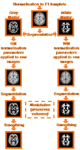
2.1.2 Processing of structural data ... 42

2.1.2.1 Segmentation ... 44

2.1.2.2 Normalisation ... 47

2.1.2.3 Customised templates ... 51

2.1.2.4 Modulation... 52

2.1.2.5 Smoothing ... 53

2.1.2.6 Statistical threshold for mass-univariate analyses ... 54

2.2 Choice of sample size in VBM: a simulation study ... 57

2.2.1 Layout of the study ... 59

2.2.2 Results of the simulation study... 62

2.3 Application of VBM to a clinical study: grey matter decrease in the early stages of anorexia nervosa in adolescents ... 66

2.3.1 Neuroimaging studies on Anorexia nervosa ... 67

2.3.2 Experimental design ... 68

2.3.2.1 Subjects and clinical procedures ... 68

2.3.2.2 MRI acquisition ... 69

2.3.2.3 Processing and statistical analyses of grey matter ... 70

2.3.2.4 Global and local volume of grey matter ... 71

2.3.2.5 Correlation analyses... 71

2.3.3 Results ... 72

(4)

2.3.3.2 Global volume changes ... 73

2.3.3.3 Regional distribution of GM changes ... 74

2.3.3.4 Region-specific GM changes ... 76

2.3.3.5 Correlations between GM changes and clinical variables in AN-r patients ... 77

2.3.3.6 Further results ... 79

2.3.4 Discussion of the results of the AN-r study ... 86

CHAPTER 3: FUNCTIONAL MAGNETIC RESONANCE IMAGING ... 93

3.1 Principles of fMRI... 94 3.1.1 Applications of fMRI ... 96 3.1.2 Physiological principles ... 98 3.1.3 Experimental paradigms ... 103 3.1.3.1 Block designs ... 105 3.1.3.2 Event-related designs ... 106

3.1.4 Preparing fMRI data for statistical analysis ... 108

3.1.4.1 Realignment ... 110 3.1.4.2 Slice-timing correction ... 114 3.1.4.3 Coregistration ... 115 3.1.4.4 Normalisation ... 118 3.1.4.5 Smoothing ... 119 3.1.4.6 Intensity normalisation ... 119 3.1.4.7 Temporal filtering ... 120

3.1.5 Statistical analysis of fMRI data ... 121

3.1.5.1 The general linear model ... 121

3.1.5.2 Independent component analysis of fMRI data ... 126

3.1.6 Systems for subject stimulation ... 130

3.2 An example application: motor planning... 134

3.2.1 A motor planning task ... 134

3.2.2 The Tower of London task ... 136

3.3 fMRI for the pre-surgical assessment of language function in drug-resistant epilepsy patients ... 143

3.3.1 The role of the lateralisation index ... 145

3.3.2 An experimental protocol for identifying eloquent regions and computing the lateralisation index ... 147

3.3.3 EEG-fMRI ... 155

3.3.4 Simultaneous EEG-fMRI recording with a reduced set of electrodes ... 159

CHAPTER 4: NEUROIMAGING AND ROBOTIC TRAINING IN NEUROREHABILITATION ... 165

4.1 Brain plasticity and neurorehabilitation ... 166

4.2 Robot-mediated therapy for motor recovery ... 169

4.2.1 The MIT-Manus robotic device ... 172

4.3 Congenital and acquired hemiparesis in children ... 174

4.4 Neuroimaging and robotic training: rationale and relevance of the research ... 176

4.5 Preliminary fMRI study on healthy adults ... 179

4.5.1 Introduction to the preliminary study ... 179

4.5.2 Experimental design ... 185

4.5.2.1 MRI data acquisition... 188

4.5.2.2 fMRI data analysis ... 188

4.5.3 Results ... 190

4.5.3.1 Subjects’ performance ... 190

4.5.3.2 Observation of arm movements and cue trajectories ... 190

(5)

4.5.4 Discussion of the results ... 198

4.6 Upper limb robot-mediated therapy and neuroimaging in children with hemiparesis ... 202

4.6.1 Design of the study ... 202

4.6.1.1 Inclusion criteria ... 202

4.6.1.2 Subjects assessment ... 203

4.6.1.3 Rehabilitative training ... 204

4.6.1.4 Neuroimaging assessment protocol ... 205

4.6.2 Preliminary results ... 207

CONCLUSIONS ... 213

LIST OF ABBREVIATIONS ... 216

(6)

________________________________________________________________________

INTRODUCTION

Magnetic resonance imaging (MRI) is considered the most important medical imaging advance since the introduction of X-rays and has assumed a role of unparalleled importance in diagnostic medicine and in basic research. MRI provides a good spatial resolution and high contrast between soft tissues of the body, which makes it especially useful in imaging the brain. A variety of properties may be used to generate different types of MR images by varying the scanning parameters. Therefore, a collection of techniques exist that enable many aspects of the structure, biochemistry, and function of the human brain to be investigated.

The present work is focused on the application of two MR neuroimaging techniques in children and adolescent patients and in healthy adult subjects. Voxel-based morphometry (VBM) was used to investigate the anatomical correlates of pathologic conditions, while functional magnetic resonance imaging (fMRI) was applied to study brain function.

VBM is an objective morphometric technique used to study neuroanatomical differences between groups of subjects, without a priori hypotheses about their localisation. It allows answering the question whether a group of subjects shows specific structural features that could be related to a pathologic condition or to a common characteristic of the group. VBM has been successful in characterising structural brain abnormalities in a variety of diseases. Furthermore, several VBM studies in groups of healthy subjects have shown structural changes at the macroscopic level, thus challenging the traditional view that the acquisition of new skills only impacts on brain function.

(7)

INTRODUCTION _

________________________________________________________________________ II

Following these results, recent studies provided evidence of structural neuroplasticity in patients after a rehabilitative training.

fMRI allows non-invasively observing the human brain at work and linking brain structure and function. During the last two decades, it has had a major impact in cognitive neuroscience and has been used in research studies on a number of diseases and disorders and on the recovery of brain function. Despite still in the earliest stages of translation from research laboratories to clinical applications, fMRI has also a growing role in clinical neuroimaging. A drawback of this technique is that it does not directly detect the electrical activity of neurons, nor does it measure the rapid increase in metabolism. Instead, fMRI indirectly estimates neuronal activity by recording an MR signal related to brain haemodynamics. However, fMRI opens an array of opportunities to advance understanding of the organisation of brain functions in healthy subjects and in those in disease states.

The research projects in which both VBM and fMRI were applied also involved the combined use of further approaches and technologies, notably electroencephalography (EEG) for EEG-fMRI coregistration and robotic devices for robot-mediated therapy (RMT).

Research involving pediatric populations, both with VBM and fMRI, is less common than studies in adults, but it represents a growing field of inquiry that is generating a rapidly expanding body of knowledge about the development of brain structure and cognitive processes in children. The non-invasive nature of MRI allows performing longitudinal analyses, which are useful in studies on brain recovery and on the development of cognitive functions in child populations. However, there are many specific issues to consider when MRI is applied in children. Some aspects of brain development continue to progress in childhood. Many physical changes are associated with the process of brain maturation, including synaptogenesis and pruning, alterations in grey matter thickness, and increases in white matter volume,

(8)

INTRODUCTION _

________________________________________________________________________ III

which can cause regional and global variation in brain structure across children of different ages and with various neurologic and developmental disorders. This process of development has many important implications. In addition to these physical changes, normal patterns for cognitive processes associated with specific tasks may change depending on the developmental level of the child. For example, some cognitive studies show that the extent of functional activation for a given task is often larger for younger children and becomes more focal as development progresses. fMRI requires subject cooperation and depends on patient’s attention which may affect the haemodynamic response, thus producing a relevant variability of activations between subjects and in repeated exams in the same subject. Therefore, patient sedation in case of anxiety or claustrophobia, which are more frequent in young children than in adults, is not possible. This may result in subject’s movement, which in turn reduces signal-to-noise ratio in fMRI images and, if it is stimulus-correlated, can introduce artefacts in the activation maps. Data processing methods can remove some movement artefact; however studies with children are sometimes compromised by excessive movement. Designing appropriate tasks for a child’s developmental level is also critical. Paradigms that are too easy may result in little activation. Tasks that are too hard may cause a child to give up. Therefore, the age and condition of the child to be scanned is an important consideration for successful fMRI task completion. However, by gearing paradigms to each child’s developmental level, it becomes difficult to make group generalisations and comparisons across these graded tasks.

The present work is divided into 4 Chapters.

Chapter 1 presents the principles of MRI. The mechanisms of data acquisition are described, together with basic imaging sequences. An overview of neuroimaging technologies and techniques is also provided in this Chapter. Computational neuroanatomy approaches for exploring brain structure in cross-sectional and longitudinal studies are briefly introduced. A summary

(9)

INTRODUCTION _

________________________________________________________________________ IV

description is also given of the differences between the physiological principles on which invasive and non-invasive functional techniques are based, together with the strengths and weaknesses of each technique.

Principles and applications of VBM are examined in Chapter 2, where details are provided on the processing of structural data (including segmentation, normalisation and use of customised templates) and on mass-univariate analyses for statistical parametric mapping.

Recruiting large groups of patients in pediatric trials can take several months or years, depending on the pathology under investigation. The issue of the number of subjects that should be included for VBM studies to provide reliable results is addressed and a simulation study intended to provide guidelines for recruiting subjects is presented. The simulation study also assesses the effects of including outliers in VBM analyses, i.e. subjects that have different anatomical characteristics from the group in which they are included.

In close collaboration with a team of neuropsychiatrists and neuroradiologists of Bambino Gesù Children’s Hospital, VBM was applied to a clinical study in a group of adolescent patients with anorexia nervosa. The characteristics of the subjects included in the study allowed searching for brain areas possibly involved in the early stages of the illness. Results of this study showed a significant global reduction of grey matter in anorexia nervosa patients, compared to control subjects. Furthermore, a region-specific reduction of grey matter was found in brain areas known to participate in mental processes related to the pathology. The latter result may indicate a greater vulnerability of these regions that could play a role in the pathophysiology of the disease and may explain the presence of a distorted body image in anorexia nervosa patients.

Chapter 3 discusses principles and applications of fMRI. This technique depends on several factors. Exam paradigm (i.e. the stimulus sequence), data processing pipeline (i.e., the sequential combination of spatio-temporal image

(10)

INTRODUCTION _

________________________________________________________________________ V

processing steps) and statistical analysis of data are all relevant aspects for the outcome, both for single subject and group studies. Strategies for controlling movement artefacts and for coregistering images from different acquisition modalities are examined, together with the general linear model for the statistical analysis of pre-processed data. Overviews are also provided of MR-compatible stimuli-delivery systems and of the fMRI experimental setting of the Imaging Department of Palidoro at Bambino Gesù Children’s Hospital. Paradigms for preliminary studies on motor planning implemented with this experimental setting are presented as example applications of fMRI.

The cumulative incidence of epilepsy in children is approximately 1% and in 30÷40% of cases drug-resistant forms are present, often eligible to be surgically treated. Indeed, neurosurgery can prevent the deleterious effects on cognitive development that are evident in some forms of childhood epilepsy. The pre-surgical mapping of brain functions allows predicting the likelihood of post-surgical deficits and to spare tissue that, if injured, would cause new clinical deficits or limit good recovery. fMRI may represent a helpful tool to localise cerebral functions in tissue within or near regions intended for neurosurgical resection of epileptic foci. Furthermore, fMRI can be used to non-invasively investigate lateralisation, which has proven useful to study organisation of cognitive functions in children and for pre-surgical evaluation of patients with medically intractable epilepsy. For such reasons, an experimental protocol for the localisation of language and motor functions and the assessment of functional lateralisation was designed. The protocol consists in a set of tasks that are likely to be easy to perform for children and impaired subjects. Furthermore, a tool was designed and implemented both to determine the dominant hemisphere and to provide the lateralisation of brain functions in specific regions of interest. A preliminary study was carried out on healthy adult subjects with the aim of providing a set of reference values for the analysis of lateralisation in children with drug-resistant epilepsy.

(11)

INTRODUCTION _

________________________________________________________________________ VI

In recent years there has been an increase of interest in the multimodal approach to the study of neuroscience due to the advantages provided by the combined use of non-invasive functional imaging tools and traditional neurophysiological techniques. In particular, simultaneous EEG and fMRI recording has overcome the inherent limitations of individual techniques, allowing localisation of the generators of functional changes that underlie specific events. The interest in this tool is supported by its potential clinical applications for the pre-surgical localisation of ictal foci. The goal is to identify regions of the brain that show signal changes immediately following epileptic spikes. However, despite the promising results from leading centres, several aspects of the combined approach are still being investigated. A preliminary study was carried out, in collaboration with a team of neurologists at Bambino Gesù Children’s Hospital, to set up the simultaneous EEG-fMRI recording technique. A substantial reduction of the MR-induced artefacts on the EEG was obtained and the quality of fMRI images was fully preserved. However, wearing conventional EEG caps used in EEG-fMRI recordings may be particularly problematic in children. Therefore, the use of a reduced set of electrodes was also explored, by testing a prototype. The results obtained showed that when the interest is in detecting when an event happens, and in localising the corresponding neuronal activations with fMRI, a reduced set of electrodes could be preferred to standard EEG caps.

An issue dominating the current debate in the field of rehabilitation concerns with the nature of functional recovery after brain injury. The recovery of motor function has been partly attributed to adaptive functional reorganisation within the central nervous system. Therefore, current rehabilitation models seek to stimulate functional recovery by capitalising on the inherent potential of the brain for positive reorganisation. Studies suggest the potential modulative effects of focused, intensive rehabilitative training in facilitating the use-dependent reorganisation. With the use of fMRI,

(12)

INTRODUCTION _

________________________________________________________________________ VII

rehabilitation therapy-induced adaptive reorganisation has been investigated. Nevertheless, the correlates between motor functional gains and changes in brain organisation are still a matter of debate. VBM studies investigated the impact of learning and practice on brain structure and studies on healthy subjects with this technique have challenged the traditional view that the acquisition of new skills only changes the way the brain functions, by showing structural changes at the macroscopic level. Recently, evidence was also provided of structural neuroplasticity resulting from rehabilitative therapy. New technologies such as robotics and virtual reality are increasingly placing side by side traditional rehabilitation treatments to assist, enhance and assess motor training. The role of these technologies within therapeutic treatment programs has been a very active area of research in recent years and is currently under debate. However, the potential of RMT and virtual reality in rehabilitation has not been extensively investigated with neuroimaging tools yet. Moreover, few studies on RMT have been conducted with patients in developmental age, when there is a bigger window for neuronal plasticity and the expected functional recovery could be better. The Movement Analysis and Robotics Laboratory (MARLab) of Bambino Gesù Children’s Hospital is the first organisation worldwide using robotic instrumentation in clinical protocols.

Chapter 4 is focused on a project developed in collaboration with a team of neurorehabilitators and neuropshycologists of the MARLab. The research is aimed at applying neuroimaging techniques to explore the effectiveness of motor RMT protocols on the recovery of upper limb deficits in children affected by congenital or acquired hemiparesis. Furthermore, it aims at comparing RMT to traditional rehabilitation techniques. VBM and fMRI are used to detect potential anatomical and functional cerebral plasticity induced by rehabilitation and underlying the recovery of upper limb motor performance. This would provide an objective means for proving or refuting the greater effectiveness of RMT, when compared to traditional therapy. The final goal is to obtain specific

(13)

INTRODUCTION _

________________________________________________________________________ VIII

indications on the most effective rehabilitation protocols for children with hemiparesis based on clinical evidence. The results of the research could also expand our knowledge on how the human brain recovers or improves impaired motor skills after brain damage in developmental age. Pediatric patients with mild to moderate upper extremity hemiparesis, clinically stable and able to participate in a RMT program, are taking part in this longitudinal study. Clinical evaluations based on standard functional scales, neuropsychological assessment, robot-based measurements, and MRI exams (fMRI tasks implemented for this study and T1 sequences for VBM analyses) are performed at the enrolment and completion of the rehabilitative training. Children are randomly assigned to receive a traditional rehabilitation therapy or a treatment with the two degrees-of-freedom planar InMotion2 robot used at the MARLab for upper limb rehabilitation. However, owing to the effort required by the training protocol (lasting 4 weeks for each subject), only very preliminary results are presented for this study.

In preparation for the application to hemiplegic children, a preliminary study was carried out on healthy adult subjects. A visual fMRI protocol was set up, able to detect a neuronal network associated with upper limb robotic training with the InMotion2 robot. The fMRI task was designed to identify the neuronal activation patterns associated with processing (observation, analysis, and representation) of human and abstract object movements similar to those executed and observed during robotic training. The subsequent aim was to verify commonalities and differences in the brain networks able to process upper limb gestures and abstract object movements, i.e. to assess the brain’s ability to assimilate abstract movements to human motor gestures. This analysis is useful to test the effectiveness of the non-biological visual feedback provided to patients during robotic rehabilitation, with respect to human movement observation, in activating brain networks for motor processing.

(14)

________________________________________________________________________

CHAPTER 1: Principles of Magnetic

Resonance Imaging

(15)

CHAPTER 1 Principles of Magnetic Resonance Imaging

________________________________________________________________________ 2

1.1 Basic principles of MRI

Nuclear magnetic resonance (NMR) is a physical phenomenon in which magnetic nuclei in a magnetic field absorb and re-emit electromagnetic radiation. This energy is at a specific frequency which depends on the strength of the magnetic field and the magnetic properties of the material that is being examined. This property can be used to record the signals emitted when the nuclei are excited at the resonance frequency.

Magnetic resonance imaging (MRI) makes use of the property of NMR to image nuclei of atoms inside the body. It is a medical imaging technique used in radiology to visualize detailed internal structures and to distinguish pathologic tissue from normal one. Any nucleus with a net nuclear spin could potentially be imaged with MRI. Such nuclei include 3He, 13C, 19F, 17O, 23Na, 31P and 129Xe. However, hydrogen is the most frequently imaged nucleus in MRI because it is present in biological tissues in great abundance (in water molecules, as well as in proteins and lipids), and because its high gyromagnetic ratio gives a strong signal. Therefore, most MR techniques are based on the acquisition of the radio frequency (RF) energy from hydrogen protons, while 13C, 19F, 23Na, and 31P are currently used in research studies more than for clinical purposes. As the result of a combination of the naturally occurring proportions of these nuclei in the body and the lower intrinsic NMR sensitivity, studies with these latter species suffer from relatively low levels of signal to noise ratio (SNR) and resolution. However, they can provide important information about biochemical and metabolic processes.

MRI is a relatively new technology. In the 1950s, Herman Carr reported on the creation of a one-dimensional NMR image. In 1971 Raymond Damadian reported that tumours and normal tissue can be distinguished in vivo by NMR and suggested that these differences could be used to diagnose cancer. While

(16)

________________________________________________________________________ 3

researching the analytical properties of NMR, in 1972 he discovered the NMR tissue relaxation differences and described the concept of whole-body NMR scanning. However, he did not describe a method for generating pictures from such a scan or precisely the characteristics that such a scan should have. Paul Lauterbur expanded on Carr’s technique and developed a way to generate the first two-dimensional (2D) and three-dimensional (3D) MRI images using gradients. In 1973, Lauterbur published the first NMR image and the first cross-sectional image of a living mouse was published in 1974. Subsequently Peter Mansfield developed a mathematical technique that would allow scans to take seconds rather than hours and produce clearer images than Lauterbur had. Damadian, along with Larry Minkoff and Michael Goldsmith, subsequently went on to perform the first MRI body scan of a human being in 1977. Paul Lauterbur and Sir Peter Mansfield were awarded the 2003 Nobel Prize in Physiology or Medicine for their discoveries concerning magnetic resonance imaging (the award was vigorously protested by Raymond Damadian). The Nobel citation acknowledged Lauterbur’s insight of using magnetic field gradients to determine spatial localisation, a discovery that allowed rapid acquisition of 2D images. Mansfield was credited with introducing the mathematical formalism and developing techniques for efficient gradient utilisation and fast imaging.

MRI is considered the most important imaging advance since the introduction of X-rays by Conrad Röntgen in 1895. Since its introduction in the clinic in the 1980s, it has assumed a role of unparalleled importance in diagnostic medicine and more recently in basic research (Logothetis, 2008). It provides a good spatial resolution and high contrast between the different soft tissues of the body, which makes it especially useful in imaging the brain compared with other medical imaging techniques such as Computed Tomography (CT). Unlike CT scans, MRI uses non-ionizing radiation and is

(17)

________________________________________________________________________ 4

harmless to the patient. Therefore, this technique is currently widely used in medical imaging.

Unlike other imaging modalities, MRI is a collection of techniques that enable many aspects of the structure, biochemistry, and function of the brain to be identified (Kuzniecky and Jackson, 2005). There are a number of choices that have to be made by the operator in order to acquire the most relevant information. Today, several MRI techniques are being used in the field of medical imaging. Examples include MR spectroscopy, diffusion MRI, MR angiography, arterial spin labelling, and functional magnetic resonance imaging, to mention only some of the most frequently used. MRI scanners are among the most complex and expensive medical technologies: the acquisition cost for a 1.5 T or 3 T scanner for medical diagnosis is currently 106> €.

1.1.1 Principles of data acquisition

1.1.1.1 Static magnetic field

The basis of MRI is the directional magnetic field associated with nuclei containing an odd number of protons and/or neutrons. Because nuclei are charged particles with a precession motion, they produce a small magnetic moment. When no external magnetic field is applied, the magnetic moments of the particles are oriented in a random manner. However, when a human body is placed in a large magnetic field, many of the free hydrogen nuclei align themselves with the direction of the magnetic field and precess about this direction like gyroscopes. This behaviour is termed Larmor precession. The frequency of precession of magnetic moments around the axis of an external magnetic field (called the Larmor frequency, ω0) is proportional to strength of

(18)

________________________________________________________________________ 5

(1.1)

where γ is the gyromagnetic ratio and B0 is the strength of the magnetic

field. The gyromagnetic ratio is nuclei specific (for hydrogen, γ=42.6 MHz/T), however, it is influenced by the molecular environment surrounding the nuclei. That is, the effects of the local environment of the molecule act to alter the effect of the applied magnetic field at the nucleus (e.g. hydrogen protons in fat molecules have different γ values from those in water molecules). Given a certain B0 static field, the frequency variation determined by a different γ value

is called the chemical shift.

Two discrete possibilities exist for the direction of precession: one for the nucleus aligned along the direction of the external magnetic field and another one in the opposite direction (anti-aligned). These two states are referred to as parallel and anti-parallel states. The parallel state is slightly lower in energy than the anti-parallel state. More nuclei occupy the lower energy than the higher energy state, thus producing a net magnetisation vector. Clinical MRI scanners use powerful magnetic fields, with field strengths between 0.1 and 3 T and even more, depending on the application (while the strength of the earth’s magnetic field is about 50 μT, i.e. about 2,000 to 60,000 times smaller). However, even with these strong fields, the excess of protons in the parallel state is only a few parts per million. Although the magnetisation effect is small, the natural abundance of protons makes the cumulative magnetisation sufficiently large to be measurable. The parameter describing the contribution of protons to the net magnetisation vector is proton density (ρ), which is one of the 3 main parameters used to contrast between different tissues (the remaining 2 parameters are the relaxation times, which will be described later).

The stronger is the B0 field, the larger will be the density of protons

(19)

________________________________________________________________________ 6

Therefore, ever stronger static magnetic fields are being produced for MRI scanners. The static magnetic field can be obtained with permanent magnets, electromagnets, or superconducting magnets. Currently, most scanners use a large coil of superconducting wire, to produce homogeneous static magnetic fields of 1> T (i.e. 10,000> Gauss). These scanners are far less power consuming than electromagnets, while the operating expenses of a superconducting magnet come from maintenance of the cooling agents, or cryogens (newer systems use liquid helium and a cold-head compressor). The superconducting magnet consists of a solenoid of wire, typically made of niobium-titanium, tightly wound to form a solenoid or cylinder around the bore of the magnet. When a constant current flows through the wire, a static, relatively uniform magnetic field is generated within the bore of the magnet, aligned in the direction of the bore. At room temperature, niobium-titanium has normal resistance. However, when it is cooled to less than 9.5 K, it becomes superconducting. Once a superconducting magnet is ramped up and fully installed, it is always on. It is essential that the main magnetic field is as homogeneous as possible, as small variations in the magnetic field are used to encode spatial position. For this reason, inhomogeneities (e.g., caused by metal) will grossly interfere with image quality. The inhomogeneity of a field is typically described in parts per million. Additional coils (known as shim coils) are used to improve the field homogeneity over the area of imaging. Shimming is particularly important after a subject is introduced into the magnet bore because the presence of the body distorts the magnetic field.

The magnetic field directed along the main axis, or bore, of the magnet usually defines the z axis. Magnetisation along the bore is referred to as longitudinal magnetisation, while that perpendicular to the bore is called transverse magnetisation. Because of the symmetry of magnetisation in the transverse plane, the x and y directions are interchangeable. By convention, 3D magnetisation vectors M are therefore considered in terms of their longitudinal

(20)

________________________________________________________________________ 7

(Mz) and transverse (Mxy) components. The angle of the vector M with respect to

the z axis, α, is referred to as the flip angle.

1.1.1.2 Radiofrequency excitation

The longitudinal magnetisation of protons in a given tissue is very small when compared to the static magnetic field B0 of the MRI scanner, so the net

magnetisation vector cannot be measured at steady state. It is therefore necessary to modify this equilibrium condition. The steady state can be perturbed by exciting protons with a brief application of a RF pulse generated by a transmitting coil, i.e. with a pulse of oscillating magnetic field that is itself precessing at the fundamental precessional frequency of the nuclei.

The energy difference between parallel and anti-parallel energy state is directly related to the precessional frequency through the following equation:

(1.2)

where h is the Planck’s constant and f is the precessional frequency, related to the Larmor frequency, ω, through:

(1.3) Thus, transitions from the parallel to the anti-parallel state can be induced in the sample when it is excited with electromagnetic radiation of energy ΔE. This energy is about 1.75x10-7 eV for a proton in a 1 T field, a tiny amount of energy compared with electron binding energies. The energy difference between the nuclear spin states corresponds to a RF photon, i.e. the energy of electromagnetic radiation in the RF region of the electromagnetic spectrum. So,

(21)

________________________________________________________________________ 8

if a tissue sample was placed in a magnetic field of 1 T and RF waves at 42.58 MHz were beamed into it, protons would be excited from the parallel to the anti-parallel state. The RF pulse represents a weak magnetic field, called B1, which

needs to be oriented perpendicular to B0 for the energy to be efficiently

absorbed. B1 tilts the net magnetisation away from the direction of the bore of

the magnet. Two processes occur simultaneously during absorption of the radiant energy:

1. reduction in longitudinal magnetisation (Mz): some of the protons resonate

and move to the anti-parallel state, resulting in a reduction in the longitudinal magnetisation;

2. phase coherence: the vectors align with each other in phase.

The outcome of phase coherence is the establishment of a net magnetic vector in the transverse plane, called the transverse magnetisation (before the RF pulse, the phases of spins were random and the magnetisation vector in the transverse plane was null). So, once longitudinal magnetisation is established by placing a patient in the magnet of an MRI scanner and radio waves at the resonant frequency are generated, we establish a transverse magnetisation while reducing the longitudinal magnetisation.

Once the RF pulse has excited the protons, tipping their magnetisation toward the transverse plane, the transmitting coil is turned off. The magnetic moments are exposed again only to the static B0 magnetic field and the

magnetisation vector will tend to relax back to its equilibrium state, becoming realigned with B0. This phenomenon is referred to as relaxation. Transitions

back to the parallel state occur spontaneously over a time period which is characteristic of individual tissues and their various pathological conditions. The recovery of longitudinal magnetisation is called longitudinal or T1 relaxation and occurs exponentially with a time constant T1. The loss of phase coherence in the transverse plane is called transverse or T2 relaxation. T1 is thus associated with the enthalpy of the spin system (the number of nuclei with parallel versus

(22)

________________________________________________________________________ 9

anti-parallel spin) while T2 is associated with its entropy (the number of nuclei in phase). Therefore, transverse and longitudinal magnetisation are components of a vector with time-varying module and represent different relaxation processes.

The rotating transverse component of net magnetisation produces an oscillating magnetic field which induces a small current in the receiver coil (frequently, the same coil is used to detect the resulting signal after the excitation stage has been terminated: the coil is then called a combined transmitter-receiver coil). It should be noted that signals cannot be detected in the longitudinal plane, while the transverse magnetisation component can be measured because it is orthogonal to the B0 field. The current collected by the

receiving coil is amplified and measured as MR signal. The detected emissions produce an exponential signal called Free Induction Decay (FID). In an idealized NMR experiment, the FID decays approximately exponentially with a time constant T2, but in practical MRI small differences in the static magnetic field at different spatial locations (inhomogeneities) cause the Larmor frequency to vary across the body creating destructive interference which shortens the FID. The time constant for the observed decay of the FID is called the T2* relaxation time, and is always shorter than T2.

Typically in soft tissues T1 is around one second while T2 and T2* are a few tens of milliseconds, but these values vary widely between different tissues (and different external magnetic fields), giving MRI its high soft tissue contrast (Table 1.1). Relaxation times depend on the efficiency of energy transfer between protons and the surrounding environment, which in turn depends on the freedom of movement of the molecules. Together with proton density ρ, relaxation times allow to contrast different tissues.

(23)

CHAPTER 1 Principles of Magnetic Resonance Imaging ________________________________________________________________________ 10 T1 (ms) T2 (ms) Grey Matter 920 100 White Matter 790 92 CSF 2.400 160

Table 1.1 - T1 and T2 values of brain tissues at 1.5 Tesla.

As stated above, the time required for protons to recover the steady state longitudinal magnetisation is expressed as the time constant T1 which, at a given magnetic field strength, is a property of the examined tissue and depends on the energy transfer with the surrounding environment. Following RF excitation, it is interactions with the local environment which cause protons to lose their excess energy and return to the lower energy state with the emission of RF radiation. This is the origin of the re-establishment of longitudinal magnetisation during relaxation. This phenomenon is called spin-lattice relaxation (spin referring to the spinning proton and lattice to its local environment). The rate at which molecules can move within their environment is related to their size and hence small molecules have a low probability for interaction. This is why fluids such as cerebrospinal fluid (CSF) have long T1 values, for instance. Medium-sized molecules (e.g. lipids), in contrast, have a greater probability for interaction and exhibit relatively short T1 values. The recovery of the longitudinal magnetisation is governed by the Bloch equation for

Mz, which has the solution:

(1.4) The decay of the transverse magnetisation is governed by:

(24)

________________________________________________________________________ 11

The so-called spin-spin interactions are interactions where two nearby protons can cause each other to flip so that one changes from anti-parallel to parallel alignment, while the other changes from parallel to anti-parallel, i.e. one gains the excitation energy from the other. Phase coherence with other excited protons is lost during this exchange and the end result is a relaxation of the transverse magnetisation. This spin-spin interaction is also called T2 relaxation. Since T2 arises mainly from neighbouring protons, a higher interaction probability exists with larger than with smaller molecules. Macromolecular environments will therefore display shorter T2 values than water-based fluids, e.g. CSF. Transverse relaxation tends to happen much more rapidly than longitudinal relaxation and T2 values are therefore generally smaller than T1 values.

Paramagnetic and ferromagnetic materials have a high magnetic susceptibility. When the field strength is raised around these materials, the magnetic field distortions raise in turn. This phenomenon produces a local variation of relaxation times. Moreover, inhomogeneities are present in the main magnetic field due to scanner non-idealities. As a consequence, neighbouring protons experience different field strengths and vary their frequency of precession, thus dephasing. Thus, differently from T2, the T2* time constant takes into account the compounding effect of imperfections in the external magnetic field and of spin-spin interactions.

1.1.1.3 Spatial localisation: magnetic field gradients

To locate the sources of MR signal, spatial encoding is required. This relies on applying strong magnetic field gradients, i.e. fields that are superimposed to the static field B0 and that vary in given directions. The

(25)

________________________________________________________________________ 12

the scanner (Figure 1.1). Magnetic field intensity varies in a linear manner along the gradient application axis. By applying a magnetic field gradient along a given direction, precessional frequencies can be deliberately made to vary with position in the magnetic field. Therefore, 3D spatial information can be obtained by providing gradients along each axis:

(1.6)

Figure 1.1 – The magnetic field gradient set (source: www.magnet.fsu.edu).

Each gradient is characterised by its strength (greater or lesser field variation for the same unit of distance), direction and the moment and time of application. First of all, a slice selection gradient is used to select the anatomical plane of interest. Within this plane, the position of each point will be encoded by applying a phase encoding gradient, and a frequency-encoding gradient. The different gradients have identical properties but are applied at distinct moments and in different directions. Gradient equivalence in the three axes means that slices can be selected on any spatial plane.

The first step of spatial encoding consists in selecting the slice plane. To do this, the slice selection gradient is applied perpendicular to the desired slice plane (let’s say along the z axis). This is added to B0, and the protons present a

(26)

________________________________________________________________________ 13

resonance frequency variation proportionate to the field strength variation that they experience (see Eq. 1.1). An RF wave is simultaneously applied, with the same frequency as that of the protons in the desired slice plane. This causes a shift in the magnetisation of only the protons on this plane. As none of the hydrogen nuclei located outside the slice plane are excited, they will not emit a signal. The RF wave associated with the slice selection gradient and the adapted resonance frequency is called the selective pulse. The thickness of the slice can be varied by adjusting the bandwidth of the selective pulse and the amplitude of the slice selection gradient. Moreover, the shape of the RF pulse in time will also determine the bandwidth profile in frequency, and thus the slice profile.

The second step in spatial encoding consists in applying a phase encoding gradient (e.g., along the y axis). The phase encoding gradient intervenes for a limited time period. While it is applied, it modifies the spin resonance frequencies, inducing dephasing which persists after the gradient is interrupted and until the signal is recorded. This results in all the protons precessing at the same frequency but with different phases. The protons in the same row, perpendicular to the gradient direction, will all have the same phase. To carry out the different phase encoding steps, the gradient is applied with different, regularly incremented values.

The final step in spatial encoding consists in applying a frequency encoding gradient in the last direction (e.g. x axis), when the signal is received. This modifies the Larmor frequencies in the x direction throughout the time it is applied. It thus creates proton columns, which all have an identical Larmor frequency. When the frequency-encoding gradient is applied, the signal is digitized at regular intervals in time. Each signal sample corresponds to a given accumulation of the gradient effect: the longer the time, the longer the effect of the gradient on the spins, and the greater their phase modification.

Frequency-encoding and phase-encoding are applied so that data are spatially encoded by differences in frequency and phase. Each frequency-phase

(27)

________________________________________________________________________ 14

couple represents a xy coordinate in a given slice and the corresponding signal intensity is proportional to the chosen weighting (ρ, T1, T2). The frequency-phase space (spectral map) obtained this way is called the k-space. To go from k-space data to an image requires using a 2D inverse Fourier Transform. Assuming a proton density weighting has been adopted, the Fourier relationship between signal and spin density can be written as:

(1.7)

The easier way to fill the k-space is to use a line-by-line rectilinear trajectory. One line of k-space is fully acquired at each excitation, containing low (contrast) and high resolution information in a given direction (e.g., along the kx axis). Between each repetition, there is a change in

phase-encoding-gradient strength, corresponding to a change along the ky axis. This allows filling

of all the lines of k-space from top to bottom. During the filling of k-space, the resulting image is containing at the beginning the edge information with low contrast, then the general shape and contrast with a blur in the ky direction that

will disappear as high spatial-frequency information in the ky direction is

completed.

1.1.2 Basic acquisition sequences

The basis of MRI ability to provide an excellent contrast and resolution and/or a fast signal acquisition is the complex library of pulse sequences that medical MRI scanners include. The essential components for any imaging sequence are: 1) an RF excitation pulse, required for the phenomenon of

(28)

________________________________________________________________________ 15

magnetic resonance; 2) gradients for spatial encoding, whose arrangement will determine how the k-space is filled; 3) a signal reading, combining one or a number of echo types determining the type of contrast. The ideal MR sequence should have high spatial resolution, high SNR, no artefacts (e.g. partial volume, motion), short acquisition time, high contrast between normal tissues and between pathologic and normal tissue, and quiet pulse sequences.

The in-plane resolution is determined by the field of view and the matrix size in the frequency encoding and phase encoding directions, that is how many picture elements (pixels) we divide the area we are imaging into. A typical matrix in clinical practice is 256x256, which means that the whole image is divided, in two dimensions, into an array of this many pixels. The actual size of the pixels will depend on the field of view. The basic volume element (voxel) of MRI images is given by the product of the slice thickness and the in-plane resolution. Therefore, the voxel is the volume of tissue from which the signal in each element arises.

Usually, more than one excitation is needed to improve the SNR. For a given pulse sequence and for given pulse parameters, the SNR is directly proportional to the voxel size and the square root of the number of data acquisitions (Nex). As the noise does not add coherently (it increases by the

square root of Nex) we have:

(1.8)

with NPy number of phase encoding steps and NFx number of frequency

encoding steps. It can be seen from Eq. 1.8 that tradeoffs between certain desired aspects of the scanning procedure have to be made. For example, thinner slices improve the signal resolution in the through-slice direction but will have a lower SNR.

(29)

________________________________________________________________________ 16

Another important issue when deciding on the optimal in-plane and though-plane resolution is that of partial volumes, i.e. the mixing of signals from different tissue types within the same voxel, which leads to a blurring of the signal intensities. The smaller the voxel size, the better will be the suppression of partial volume effects. However, this will be at the cost of SNR and acquisition time.

Motion is a major problem in standard MRI pulse sequences, in which the image is acquired one phase-encoding step at a time rather than in a “single shot”. The effect of motion is significant not just because of gross head movements but also because of pulsations from blood vessels and respiration, which are intrinsic to the biologic system being imaged and may cause image ghosting.

Contrast is a direct consequence of the relative signal intensities from different tissue types. The most important contrast factors in MRI are proton density (ρ) and relaxation times (T1, T2 and T2*). For example, with particular values of the echo time (TE) and the repetition time (TR), which are basic parameters of image acquisition, a sequence takes on the property of T2-weighting. On a T2-weighted scan, water- and fluid-containing tissues are bright and fat-containing tissues are dark. The reverse is true for T1-weighted images. Other intrinsic components of the signal that can generate contrast include diffusion contrast, chemical shift, and perfusion contrast.

There is over a hundred different types of sequences, most of which may be classified in two main families, depending on the type of echo recorded: spin echo (SE) sequences (characterised by the presence of a 180° rephasing RF pulse) and gradient echo (GRE) sequences (Figure 1.2). Numerous variations have been developed within each of these families, mainly to increase acquisition speed (e.g.: fast SE, single shot fast SE, spoiled GRE, ultrafast GRE, steady state GRE, echoplanar. Some sequences are hybrid, mixing SE and GE

(30)

________________________________________________________________________ 17

(GRASE, SE-EPI). Specific sequences have been developed for MR angiography, perfusion imaging, diffusion imaging and MR spectroscopy.

Figure 1.2 – Families of spin echo and gradient-echo sequences (source: www.imaios.com).

1.1.2.1 Spin echo sequences

The SE sequence is made up of a series of events: 1) 90° pulse; 2) 180° rephasing pulse at TE/2; 3) signal reading at TE (Figure 1.3). Historically, SE was the first sequence to be used. The 90° RF pulse rotates the net magnetisation vector from the z axis to the xy plane. After the 90° pulse, the net magnetisation vector precesses on the xy plane, however, due to field inhomogeneities, single protons precess with different frequencies leading to an irreversible loss of magnetisation. This dephasing can be reversed by applying a 180° or inversion pulse that inverts the magnetisation vectors (in fact, a 180° pulse can be used to either invert the magnetisation in the z-direction or to reverse the direction of the magnetisation when it is already in the xy-plane). If the inversion pulse is applied after a period TE/2 of dephasing, protons will rephase to form an echo at time TE. The intensity of the echo relative to the initial signal is given by e−TE/T2 where T2 is the time constant for spin-spin relaxation. Therefore, the 180°

(31)

________________________________________________________________________ 18

rephasing pulse compensates for the constant field inhomogeneities to obtain an echo that is weighted in T2.

Figure 1.3 – Spin echo sequence time diagram (source: www.imaios.com).

In the classical SE sequence, this series is repeated at each time interval TR. With each repetition, a k-space line is filled, thanks to a different phase encoding, so that for a SE sequence with NPy rows, we make NPy acquisitions.

Therefore, the duration of the classical SE sequence is:

(1.9) It is of no use to acquire an image that does not have any contrast between grey and white matter, even if there is strong signal from both of them, so shortening the TR of a sequence (i.e. the time interval between two successive 90° RF waves) to reduce imaging time needs to be considered carefully.

A SE sequence has two essential parameters: TR and TE. TR conditions the longitudinal relaxation of the explored tissues (depending on T1). The longer the TR, the more complete the longitudinal magnetisation regrowth (Mz tends to

its steady state value). Reducing TR to 300÷600 ms weights the image in T1 as the differences between the longitudinal relaxations of the tissues’ magnetisation

(32)

________________________________________________________________________ 19

will be highlighted. In the T2-weighted SE sequence the TR and TE parameters are optimised to reflect T2 relaxation. When the TR is long (over 1,600÷2,000 ms), longitudinal magnetisation recovery is complete and the influence of T1 on signal magnitude will be minimised. Associated with long TE (60÷140 ms), the different tissues are better highlighted according to their T2. Long T2 tissues will appear as a hypersignal, as opposed to short T2 structures, which will appear as a hyposignal. A long TR (over 2,000 ms), associated with a short TE (10 to 20 ms) will relatively suppress both the influence of T1 and the effect of T2 on signal magnitude and the contrast obtained will depend on the proton density ρ. The major disadvantage with T2 weighted SE sequences is linked to long TR resulting in prohibitive acquisition times. While SE sequences can be used in clinical practice to obtain good quality anatomical T1-weighted images, faster types of sequence are preferred to obtain T2-weighted images.

In the classical SE sequence, the time interval between reading the echo and the new RF excitation pulse is usefulness. In fast SE sequences, multiple 180° pulses are applied to obtain a SE train. After each echo, the phase-encoding is cancelled and a different phase-encoding is applied to the following echo. This enables to use the time interval after the first echo to receive the echo train in order to fill the other k-space lines in the same slice. Because of the reduced number of repetitions (TR) required, the k-space is filled faster and slice acquisition time is reduced.

Multi-echo SE sequences allow several images of the same slice position without increasing overall acquisition time. The advantage is that the images are obtained with a different contrast, which is useful in characterising certain lesions. After the first echo is obtained, there is a free interval until the next TR. By applying a new 180° pulse, a new echo is received, with the same phase encoding, to build the second image. The echo time of the two images differs and the second image will be more T2-weighted than the first. Typically, these sequences are used to obtain simultaneously ρ- and T2-weighted images.

(33)

________________________________________________________________________ 20

Finally, in multi-section acquisition, another slice is excited during this time interval with a RF pulse at a slightly different frequency and the corresponding echo is measured. Therefore, for each TR multiple slices can be excited. Slices are usually excited in an interleaved manner to avoid cross-talk effects that could occur in case two adjacent slices were excited.

1.1.2.2 Inversion recovery

Inversion-recovery (IR) is a magnetisation preparation technique followed by an imaging sequence of the SE type. The sequence starts with a 180° RF inversion wave which flips longitudinal magnetisation Mz in the opposite

direction. Due to relaxation, longitudinal magnetisation will increase to return to its initial value, passing through null value. After an inversion time (TI), a further 90° RF pulse tilts some or all of the z-magnetisation into the xy-plane to obtain transverse magnetisation, where the signal is usually rephased with a 180° pulse as in the SE sequence. If a TI is chosen such that when the 90° pulse is applied the longitudinal magnetisation of a tissue is null, the latter cannot emit a signal (absence of transverse magnetisation due to the absence of longitudinal magnetisation). The IR technique thus allows the signal of a given tissue to be suppressed by selecting a TI adapted to the T1 of this tissue.

As longitudinal regrowth speed is characterised by relaxation time T1, IR sequences are weighted in T1. This sequence has the advantage that it can provide very strong contrast between tissues having different T1 relaxation times. IR can also be combined with sequence types other than the standard SE. In particular, it can be combined with fast SE sequences to save considerable time. However, a disadvantage of this technique is that the additional inversion RF pulse makes it less time efficient than the other pulse sequences.

(34)

________________________________________________________________________ 21

IR can be used to suppress tissues like fluid or fat. In particular, fluid attenuated inversion recovery (FLAIR) is an IR pulse sequence utilised to null signal from fluids that can be used in brain imaging to suppress CSF so as to bring out the periventricular hyperintense lesions, such as multiple sclerosis plaques.

1.1.2.3 Gradient echo sequences

The gradient echo (GRE) sequence differs from the SE sequence in regard to the absence of a 180° RF rephasing pulse and to the excitation pulse (termed the α pulse) which tilts the magnetisation by a partial flip angle between 0° and 90° (Figure 1.4).

Figure 1.4 – Gradient echo sequence time diagram (source: www.imaios.com).

As there is no 180° RF pulse, a bipolar readout gradient (which is the same as the frequency-encoding gradient) is required to create an echo. The gradient echo formation results from applying a dephasing gradient before the frequency-encoding or readout gradient. The goal of this dephasing gradient is to obtain an echo when the readout gradient is applied and the data are acquired.

(35)

________________________________________________________________________ 22

The dephasing stage of the readout gradient is in the inverse sign of the readout gradient during data acquisition. Moreover, its dephasing effect is designed so that it corresponds to half of the dephasing effect of the readout gradient during data acquisition. Consequently, during data acquisition, the readout gradient will rephase the spins in the first half of the readout (by reversing the dephasing effect of the dephasing lobe), and the spins will dephase in the second half (due to the dephasing effect of the readout gradient). Data are not acquired in a steady state, where z-magnetisation recovery and destruction by α-pulses are balanced. The magnetisation is used up by tilting a little more of the remaining z-magnetisation into the xy-plane for each acquired imaging line. The consequence of a low-flip angle excitation is a faster recovery of longitudinal magnetisation that allows shorter TR and TE and decreases scan time. On the other hand, the result of a lower flip angle excitation is a lower tipped magnetisation. As GE techniques use a single RF pulse and no 180° rephasing pulse, the relaxation due to fixed causes is not reversed and the loss of signal results from T2* effects. The signal obtained is thus T2*-weighted rather than T2-weighted. These sequences are thus more sensitive to magnetic susceptibility artefacts than are SE sequences. T2* weighting can be minimised by keeping the TE as short as possible, but pure T2 weighting is not achievable. Gradient echoes have a reduced crosstalk, so that a small or no slice gap can be used.

Proton density-weighted images can be obtained by applying a small flip angle, a long TR and a short TE; to obtain T1-weighted images a large flip angle (>70°), a short TR (less than 50 ms) and a short TE must be applied; finally, for T2*-weighted images a small flip angle, a longer TR (100 ms) and a long TE (>20 ms) are required.

(36)

________________________________________________________________________ 23

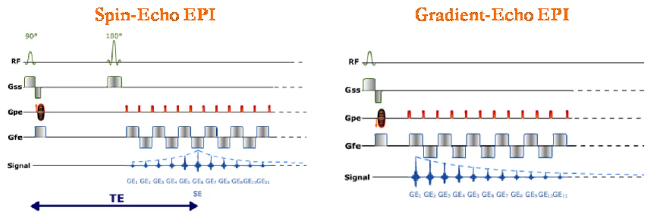
1.1.2.4 Echo Planar Imaging sequences

Echo planar imaging (EPI) is a fast acquisition sequence (tens to hundreds of ms/slice), introduced by Peter Mansfield in 1977. It is used in applications like diffusion, perfusion, and functional magnetic resonance imaging. The EPI sequence is based on: 1) an excitation pulse, possibly preceded by magnetisation preparation; 2) a continuous signal acquisition in the form of a gradient echo train, to acquire total or partial k-space (single shot or segmented acquisition, respectively); 3) readout and phase-encoding gradients adapted to spatial image encoding. In single shot EPI, the complete image is formed from a single data sample (i.e., all k-space lines are filled in one repetition time) of a GRE or SE sequence. The major drawback of EPI is the limited spatial resolution. Moreover, EPI is relatively demanding on the scanner performance, in particular on gradient strengths, gradient switching times, and receiver bandwidth (the scan time is dependent on the spatial resolution required, the strength of the applied gradient fields and the time the machine needs to ramp the gradients). In addition, EPI is extremely sensitive to image artefacts and distortions.

Contrast possibilities include GRE EPI (a single RF excitation pulse is used, with no preparation, and a T2* weighting is obtained), SE EPI (where a pair of 90°-180° pulses is used and a T2 weighting is obtained), and IR EPI (with a 180° inversion pulse to prepare magnetisation, followed by an RF excitation pulse to obtain T1 weighting). The time diagram for SE and GRE EPI sequences is shown in Figure 1.5. By periodically fast reversing the readout or frequency encoding gradient, a train of echoes is generated.

Several trajectories can be used to fill the k-space. As stated above, a readout gradient is continuously applied to constitute the echo train (a GRE train in Figure 1.6), with positive and negative alternations.