A Contrast-Based Approach to the Identification of Texture Faults

UNIVERSITY

OF TRENTO

DEPARTMENT OF INFORMATION AND COMMUNICATION TECHNOLOGY

38050 Povo – Trento (Italy), Via Sommarive 14 http://www.dit.unitn.it

A CONTRAST-BASED APPROACH TO THE IDENTIFICATION OF TEXTURE FAULTS F. G. B. De Natale, F. Granelli, and G. Vernazza

January 2002

A C

ONTRAST

-B

ASED

A

PPROACH TO THE

I

DENTIFICATION OF

T

EXTURE

F

AULTS

Francesco G. B. De Natale1, Fabrizio Granelli1, and Gianni Vernazza2 1

DIT - University of Trento Via Sommarive, 14 – 38050 Trento, Italy

Phone: +39 0461 882058 (1696 Fa x) e-mail:[denatale, granelli]@ing.unitn.it

2

DIBE - University of Genoa Via Opera Pia, 11a – 16135 Genoa, Italy

Phone: +39 010 353 2755 (2134 Fax) e-mail: vernazza@dibe.unige.it

ABSTRACT

Texture analysis based on the extraction of contrast features is very effective in terms of both computational complexity and discrimination capability. In this framework, max -min approaches have been proposed in the past as a simple and powerful tool to characterize a statistical texture. In the present work, a method is proposed that allows exploiting the potential of max -min approaches to efficiently solve the problem of detecting local alterations in a uniform statistical texture. Experimental results show a high defect discrimination capability, and a good attitude to real-time applications, which make it particularly attractive for the development of industrial visual inspection systems.

A C

ONTRAST

-B

ASED

A

PPROACH TO THE

I

DENTIFICATION OF

T

EXTURE

F

AULTS

Fabrizio Granelli, Francesco G. B. De Natale, and Gianni Vernazza

Abstract

Texture analysis based on the extraction of contrast features is very effective in terms of both computational complexity and discrimination capability. In this framework, max -min approaches have been proposed in the past as a simple and powerful tool to characterize a statistical texture. In the present work, a method is proposed that allows exploiting the potential of max -min approaches to efficiently solve the problem of detecting local alterations in a uniform statistical texture. Experimental results show a high defect discrimination capability and a good attitude to real-time applications, which make it particularly attractive for the development of industrial visual inspection systems.

1. Introduction

Automatic systems for visual inspection of materials are becoming more and more popular, due to several reasons: the increasing power of digital signal processing architectures, the affordable cost of digital image acquisition and processing systems, the availability of fast algorithms able to achieve nearly human performance in several inspection tasks. Within this field, a typical problem to be solved is the identification of defects in a raw or processed material, which can usually be assimilated to the problem of detecting an anomalous distribution of colours or grey levels in an image with known characteristics. The most challenging situation occurs when the sample to be analysed presents a patterned or textured surface: in this case, the defect would appear as a local anomaly in a regular or statistical texture.

A typical approach to this problem consists in identifying a parametric model able to represent a uniform texture, and then to define suitable techniques for system training and operation. During the training phase, the system should compute the optimum model parameters for a given texture sample. During the operation phase, the system should extract the relevant set of parameters from each input sample, and compare it with the model, in order to discriminate image areas that do not comply with the mock-up. To perform a comparison, suitable homogeneity measures should be adopted.

As to the problem of texture representation, several models have been proposed that can be adopted in the framework of discriminating different texture. They can be roughly classified into two main

groups: methods based upon spectral properties, and methods based upon spatial statistics of the texture. Gabor filters belo ng to the first category and are widely used in image processing applications where a high accuracy is required in both space and frequency domains: they have been successfully applied to the problem of texture representation and segmentation [1,2]. Other interesting approaches involve the exploitation of the multi-resolution and multi-scale properties of the wavelet decomposition, which are desirable feature in the problem of texture characterization [3,4].

Concerning techniques operating in the spatial domain, a wide variety of methods can be found in the scientific literature. Most important examples include structural methods, based on the definition of texture elements or texels and relevant construction rules [5]; approaches based on fractal geometry, where the main features used to classify different textures are the fractal or multi-fractal dimensions [6]; and statistical methods. This last class includes several significant techniques. Methods using low-order statistics (e.g., histogram-based analysis, rank-order approaches [7]) are usually rather simple and fast, but usually are not sufficient guarantee a very high accuracy. High-order statistics (e.g., co-occurrence matrices [8]), provide much more accurate models, but are characterized by huge memory and computation requirements, even if fast solutions have been recently proposed [9]. Finally, auto-regressive models (e.g., Markov Random Fields [10], and hidden MRF [11]) provide powerful tools both to describe and to synthesize statistical textures. Focusing on the problem of detection of texture faults, some specific advances were published in the literature in the last years. Even in this case, a distinction can be formulated between techniques based on spectral measurements and techniques working on spatial statistics. In [12] a comparison between the two approaches is outlined. Among spectral domain techniques, an interesting work is presented in [13], where concepts deriving from the wavelet theory are integrated with the use of co-occurrence matrices. Detection of defects is performed by decomposing the texture image into sub-bands and then partitioning the resulting images into non-overlapping sub-windows and classifying them based on a set of co-occurrence parameters.

On the other hand, statistical measures demonstrated to be successfully applicable to the detection texture faults. Higher-order statistics (HOS) are used in [14], where feature vectors consisting of hybrid combinations of second- and higher-order statistics, are classified as defective or non-defective on the basis of the Mahalanobis distance. Simpler approaches employ information extracted from the statistics of lower order: in [15] texture faults are detected through the use of an adaptive lattice filter, driven by the knowledge of the first-order statistics contained in a modified grey level histogram.

A common drawback of the approaches based on the computation of image statistics is the strict relationship between performance and complexity. In particular, co-occurrence matrices, fractals and structural approaches show a very good discrimination capability but require a huge computation, while simpler methods based on low-order statistics (e.g., histograms) are suitable for real-time implementations but show a limited reliability and accuracy. Contrast-based approaches [16, 17] are a very interesting alternative, for they do not require all the texture pixels to be taken into account in the statistics. In the max- min technique, only a set of ‘significant’ points, corresponding to the local maxima and minima (extremes) of the intensity function along one-dimensional scan lines are used for texture characterization. The advantage of such a procedure in terms of complexity reduction is twofold. First, statistical analysis is applied only to the local extremes, which are proven to be representative for the whole texture, while representing a small fraction of the total image pixels. Second, the analysis is performed on one-dimensional arrays, thus reducing the complexity to a few vector operations. Nevertheless, an in-depth study of the performance of the ‘max- min’ technique reveals that the basic method, although very effective in texture discrimination, is almost unusable with application to the problem of texture fault detection. This depends on the fact that large uniformly textured areas are needed to extract significant parameters, thus preventing the possibility of an accurate detection and segmentation of typical texture defects, which just affect small image regions.

Further stud ies lead to a modified approach, described in this paper. Here, the texture is scanned with a particular windowing procedure, and a set of features is extracted from each texture sample for the purpose of a binary classification (‘correct’ or ‘defective’ pattern). The method requires an adaptation phase, consisting in the off- line analysis of a sample texture, aimed at determining a ‘texture model’ (prototype). Then, during operation, the texture samples are analysed to verify their compliance with the model.

In the following sections, the max- min approach is briefly reviewed, the proposed algorithm is described in detail, experimental results are discussed, and finally, conclusions are drawn.

2. The Max-Min Approach

The max- min approach proposed in [16] consists of the following iterative procedure: i. extract an image scan- line and put it into a linear vector;

ii. process the vector with a non- linear smoothing filter using a threshold TS ;

iii. extract the maxima and minima of the filtered vector, count the m and store the result; iv. repeat steps (ii)-(iii) for a fixed number of iterations N.

The smoothing filter is aimed at progressively reducing the number of extremes at each step, by eliminating the less ‘significant’ ones (where the significance is related to the amplitude of the luminance variation). The following algorithm achieves it:

IF

(

xk+1 - yk > TS/2

)

THEN yk+1 = xk+1 - TS/2 ELSE IF

(

| xk+1 - yk | < TS/2

)

THEN yk+1 = yk

ELSE IF

(

xk+1 - yk < - TS/2

)

THEN yk+1 = xk+1 + TS/2

where xi and yi are the grey levels of the i-th point of the vector before and after

smoothing, and TS is a proper pre-defined threshold (see [16]). After a given number of

iterations N, a feature vector is built, given by the (N-1) ratios between the number of extremes before and after each filtering step. Such a vector provides a kind of texture signature, which can be used for classification purposes.

Tests performed on the above algorithm demonstrated that it is able to classify with good reliability different textures, given that a sufficient number of pixels is available. On the contrary, its inadequateness appears evident when applied to the identification of small-size anomalies within uniform textures. This fact can be easily verified by considering an example. Let us apply the max-min method to the two different textures in Figs. 1.a and 1.b (selected from the Brodatz album). The algorithm provides a set of features for each vector of image pixels given in input (a group of scan lines extracted from one of the textures). The intra- and inter-set Euclidean distances calculated on these feature sets confirm that the two clusters are sufficiently compact and separated to guarantee a correct classification of the texture samples (see Table I). Then, let us create a synthetic image (see Fig. 1.c) by inserting a 100×100 patch of texture 1.b in texture 1.a. Although a human observer easily perceives the presence of the anomaly, the feature vectors extracted from the anomalous scan lines do not reveal any significant variation. This is clearly visible in the chart of Fig. 2, where the distance of each scan line of Fig. 1.c from the prototype of texture 1.a is plotted. In this context, the prototype is achieved by averaging a certain number of feature vectors, extracted from “correct” scan lines.

The reason of the inefficiency of the max- min approach in this case is twofold. First, the topology of the analysed scan lines is such that only a few pixels of the defective area are included in each inspected sample, thus not sufficient to influence the global statistics. Second, the relative density of extremes at different smoothing thresholds provides an incomplete characterisation of the texture, which in turn gives highly unstable statistics if only a few samples are available, as in the case of texture fault detection.

3. Contrast-Based Feature Extraction and Defect Localization

The proposed method includes an adaptation phase (to be performed off- line) and an anomaly detection phase (on- line). The adaptation phase is aimed at generating a prototype of a regular texture, while the detection phase consists in the location of possible defects and the consequent identification of the area affected by the anomaly. This task is achieved by comparing the texture sample s with the prototype.

Both phases share a common core algorithm, which includes three main operations:

• scan a texture image with a particular windowing procedure;

• for each sample, extract the local extremes at various smoothing thresholds;

• for each local maximum or minimum, compute a set of parameters that will be used to construct the feature vector associated to the relevant sample.

In the adaptation phase, these operations are applied to a training set made up of a certain number of samples extracted from a regular texture. This operation leads to the definition of a prototype vector, calculated by averaging the feature vectors extracted from the samples themselves (i.e., computing the centroid of the cluster). In practical applications, the training set can be constructed by randomly taking some patterns from different non-defective mock-ups of the inspected material. The number of samples to be included in the training set clearly depends on the feature vector dimension (in our tests it was set equal to 10 times the number of features). If a sufficiently large acquisition of a correct texture is available, spatial sampling can be a reasonable alternative, provided that a sufficiently large number of samples can be achieved. During defect detection, the three above mentioned operations are similarly performed to compute the distance of the inspected pattern from the prototype, thus allowing to discriminate defective regions.

The following subsections offer a detailed description of the processes of texture scanning and feature extraction, which are of fundamental importance for the effectiveness of the method.

3.1 Windowing procedure

In section 2 we observed that one of the main difficulties in using the max- min approach to detect texture faults is the low percentage of defective pixels in the analysed samples, which does not allow a sufficient statistical characterisation of the local texture. A bare reduction of the scan line dimension is not an effective solution. In fact, although it leads to an increased percentage of defective points in the analysed sample, it also implies a very limited dimension of the sample, which compromises the reliability of the estimation. A better solution can be to analyse groups of consecutive scan lines, achieved by partitioning the texture in small areas to be independently processed. Nevertheless, this procedure must be carefully studied in order to avoid losing precision in defect identification.

In this work a particular texture scanning method was set up, which allows to achieve both a statistically significant sample dimension and a sufficient incidence of the defect within the analysed sample. The procedure consists in tiling the image and applying to each block a moving-window scanning procedure, consecutively performed in the x and y directions of the image plane. The choice of the block size for image tiling is strictly application-dependent, for it is connected both to the texture scale (also related to the acquisition resolution) and to the dimension of the flaws to be detected. Generally speaking, the window must contain a sufficient portion of the texture in order to be statistically significant, and possible defects should impact to a sufficient extent the analysed sample (at least 10% of the surface). In the experiments carried out, the window size was manually set, in the range 50×50÷150×150 pixels. It is also possible to set up automatic procedures for this task, for instance by analysing the statistics of a large number of fixed-size blocks extracted from a regular texture pattern, and progressively incrementing the block size until the statistical parameters converge to a constant value (spatial stationariety).

Concerning the window size, it should be set to an odd number M of block rows ranging from 3 to 7. The window is shifted by one line at a time, thus with an overlap of M-1 rows (see Fig. 3.a); for each positioning, the block rows embraced by the moving window are organised in a linear array (by a bi-directional raster scanning), from which a set of contrast features is extracted.

This procedure is applied in both training and operation phases. In the training process, every feature vector is collected independently of the window position (owing to the hypothesis of stationariety), and used to generate the texture prototype. A different prototype is created for the two spatial directions (x, y), in order to take into account possible spatial anisotropies in the texture. Samples used to generate the two prototypes can be possibly overlapped in the x and y directions. During defect detection, the window is progressively centred on the inspected line, and the relevant feature vector is used to determine the compliance of the corresponding line with the prototype. Lines that show different properties from the prototype are marked as defective, and are matched with the lines in the perpendicular direction to locate defective points, as shown in Fig. 3.b. Of course, this procedure does not produce an exact segmentation of the defect, but it allows identifying with a very good reliability the bounding rectangle that includes it.

As to the identification of defective lines, a simple threshold applied to the mean square difference (MSD) between the feature vector associated to the currently inspected line and the prototype can produce an adequate result. The adopted threshold T can be manually set up, or can be automatically determined by taking into account the dispersion of the samples in the adaptation set: to this purpose, all the patterns in the training set are used to reliably estimate the distribution of the correct texture samples. A simple solution consists in computing the distance among each sample j

in the training set and the prototype MSD(j), and setting the threshold to T=TD=max j{MSD(j)}: a

sample is then considered defective if its distance from the prototype exceeds TD. This solution is

very easy and yields good results if the training set is sufficiently homogeneous; otherwise, better results can be obtained by considering the variance of the sample distances. If σD is the standard

deviation of the MSD between the training feature vectors and the relevant prototype, good results can be achieved by setting the threshold to T=T_σ=3σD. Nevertheless, in practical applications where

a very large number of images are analysed using the same system set-up, the manual setting of the threshold (obtained through a simple user interface) can become a competitive solution.

By applying the method so far described it is possible to process images samples of 150 to 1000 pixels, depending on block and window size, which are usually adequate to achieve reliable statistics. Moreover, even for very small-sized defects (10-20 pixels in diameter), the percentage of defective points is high enough to affect the statistics of the involved samples.

3.2 Characterisation of local extremes

The example given in Fig. 2 shows that the density of local extremes at different scales is not sufficient in general to completely characterise a texture. In particular, this measure fails when different text ures are present in the analysed sample, a situation that is common in texture fault detection problems.

To increase the discrimination performance of the classifier, several parameters were initially considered, and their values computed on a large set of samples. The objective was to find significant measures, able to describe the statistical properties of the peaks and valleys (maxima and minima) that alternate in the line scanning of a texture. After normalizing the feature vector, a careful selection was accomplished by measuring the relative weight of each parameter inside the vector and the correlation factor of each pair of coefficients. The less significant coefficients were then discarded, while the correlated ones were simplified, modified or merged (when semantically admissible). At the end of this process, a set of seven parameters was defined. To build the feature vector connected to a texture sample, the values of the seven parameters are calculated at each smoothing iteration, thus generating a vector of dimension 7×N, N being the number of iterations.

The basis parameters are described hereafter:

• Density of local extremes: it is given by the ratio between the number of local extremes Nextr and the total number of pixels in the sample Npel :

pel i estr i estr i N N N d , 1,.., ) ( ) ( = = (1)

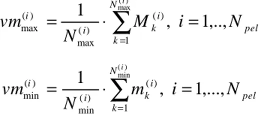
• Expected value of local maxima Mk and minima mk: it is the mean value of the grey levels associated to the extremes, independently calculated for maxima (peaks) and minima (valleys): pel N k i k i i N i M N vm i ,.., 1 , 1 max() 1 ) ( ) ( max ) ( max = ⋅

∑

= = pel N k i k i i N i m N vm i ,..., 1 , 1 (min) 1 ) ( ) ( min ) ( min = ⋅

∑

= = (2)

• Variance of local maxima and minima: it is the mean square deviation of the grey levels associated to the extremes from the corresponding expected values:

∑

₌ − = ⋅ − = ) ( max 1 2 ) ( max ) ( ) ( max ) ( max ( ) , 1,.., 1 1 var i N k pel i i k i i N i vm M N

∑

= = − ⋅ − = ) ( min 1 2 ) ( min ) ( ) ( min ) ( min ( ) , 1,..., 1 1 var i N k pel i i k i i N i vm m N (3)

• Power of peaks and valleys : it is the mean value of the peaks/valleys power, defined as the square sum of the differences between the grey levels xi of the pixels belonging to the peak/valley and the basis k of the relevant peak/valley (i.e., the minimum grey level for peaks and the maximum grey level for va lleys):

pow m m x k peak l i i m m = − ⋅ − =

∑

1 2 1 2 1 2 ( ) ⇒⇒ pow N pow i i peak l l Ni max ( ) max ( ) max( ) = =

∑

1 1 pow M M k x v l i i M M alley = − ⋅

∑

= − 1 2 1 2 1 2 ( ) ⇒⇒ pow N pow i i v l l N i min ( ) min ( ) min ( ) = =

∑

1 1 alley (4)

Fig. 4 provides a graphical representation of the various elements used to compute the above parameters, sketched on a sample scan line.

4. Analysis of Computational Complexity

One of the main goals of the proposed method is to develop a technique able to reliably detect texture faults with very little needs in terms of hardware and computation. This is a very desirable feature in many industrial systems that require low-cost and nearly real-time image analysis tools (e.g., the visual inspection of materials in a production line). In this section, the computational complexity of the method is analysed in detail to demonstrate the viability of the proposed approach from this viewpoint also.

To this aim, the number of elementary operations (sums, products, and comparisons) to be executed for each image pixel is calculated. Since the complexity strictly depends on the number

of extremes found in a scan line, we considered the worst case, consisting in a continuous alternation of maxima and minima. Based on a sample dimension of Npel pixels, and neglecting

the operations not depending on Npel (Npel >> 1), one needs, for a single smoothing threshold:

- N_pel comparisons to determine local extremes (maxima and minima); -

2 pel

N

sums to calculate the density of maxima;

- 2

pel

N

sums to calculate the mean value of maxima;

- 2 pel N products and 2 pel N

sums to compute the variance of maxima;

- 2

pel

N

products and N_pel sums to compute the power of maxima;

An equal number of elementary operations are required for the computation of parameters relevant to local minima. Summarizing the above data, and multiplying for the number of thresholds N adopted in the iterative smoothing procedure, we achieve:

   ⋅ ⋅ ⋅ ⋅ products N N s comparison and sums N N pel pel 2 7

Finally, we have to consider that the texture analysis is applied as a sliding window and the scanning is sequentially operated in the horizontal and vertical directions. Then, the above operations are performed 2M times for each pixel, where M is the window size (number of block rows that forms a texture sample). The expression we obtain is the number of operations for a texture sample, which must be further divided by Npel to achieve the number of elementary

operations per pixel:

   ⋅ ⋅ ⋅ ⋅ products N M s comparison and sums N M 4 14

We should take into account the normalization and the computation of the distance from the prototype, but the relevant number of operations is negligible as compared to the above, being

Npel >> 1. It can be observed that the order of complexity is linear with the dimension of the

window, which is usually quite small. Furthermore, this number is largely overestimated, being the number of local extremes typically much lower than Npel and rapidly decreasing with the

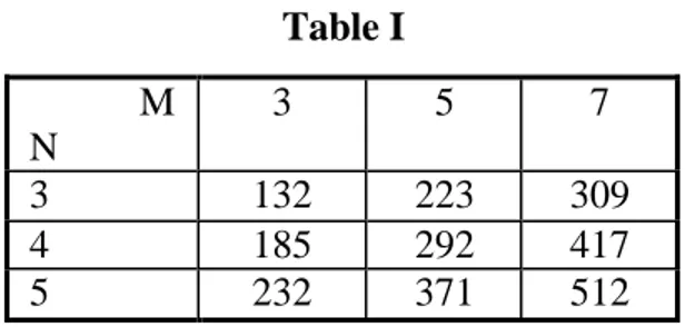
smoothing iterations. Table I shows the time spent (in msec) to process a 512x512 b/w texture image, for some typical parameter settings: simulations were performed on a Sun Spark Ultra 80 workstation running Sun-Solaris operating system. Furthermore, the algorithm enjoys a very high degree of parallelism that makes it suitable for fast DSP implementation.

5. Experimental Results

Several simulations were carried out to verify the effectiveness of the proposed approach. In order to validate the performance of the algorithm on a controlled environment, the method was first tested on a set of 10 synthetic images, obtained by including small extraneous patches in a homogeneous texture pattern, as already shown in Fig. 1. The textures used to build this set were selected from the Brodatz collection, by previously equalizing the average grey level in order to avoid biasing the result.

The chart in Fig. 5 allows evaluating the discrimination capability of each feature in the analysis of the defective test image of Fig. 1.c. In particular, each curve plots the distance between horizontal texture samples and prototype (extracted from the texture of Fig. 1.a) for a specific feature. It is possible to observe that in this case the power of peaks is the dominant feature. Fig. 6 shows the distance between each horizontal sample and the prototype, calculated on the overall feature vector. A direct comparison between the charts in Figs. 2 and 6 makes evident that the proposed method provides dramatically better discrimination capabilities: in fact, it is now possible to clearly identify the defective area (extraneous patch) and segmenting the flaw by a unique threshold. This result was achieved by directly processing the entire texture 512x512 pels without tiling (due to the very large size of the “defect”), setting the window size to M=3 rows (columns), and using N=4 smoothing iterations. Therefore, each analysed sample had a size of 1536 pixels, and was represented by a feature vector of dimension 28; anomalous samples contained 300 pixels of the extraneous texture, equal to 20% of sample dimension.

A quantitative performance index was also defined in order to better evaluate the results achieved. It simply consists in the percentage image area that is wrongly classified by the system (pixels belonging to the extraneous patch that are not detected, and pixels belonging to the main texture classified as faulty). The average error rate computed on the entire synthetic test set was equal to 2.6%, with all the errors concentrated on the borders of the defective area and no correct areas classified as defective (false alarms rate = 0).

In a second phase, the method was tested on a large set of natural images, including textured ceramic tiles and ornamental stones (granite tiles). The adopted test set was acquired in the framework of some industrial grants targeted to the definition of suitable technologies for automatic visual inspection of construction materials. It includes over 300 images with different types of defects (cracks, blobs, stains and other imperfections) over differently textured natural and synthetic materials. Also in these conditions, the performance of the proposed method was very satisfactory, as confirmed by the following examples.

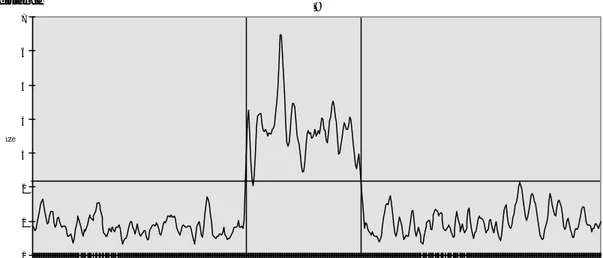
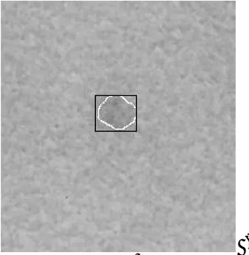
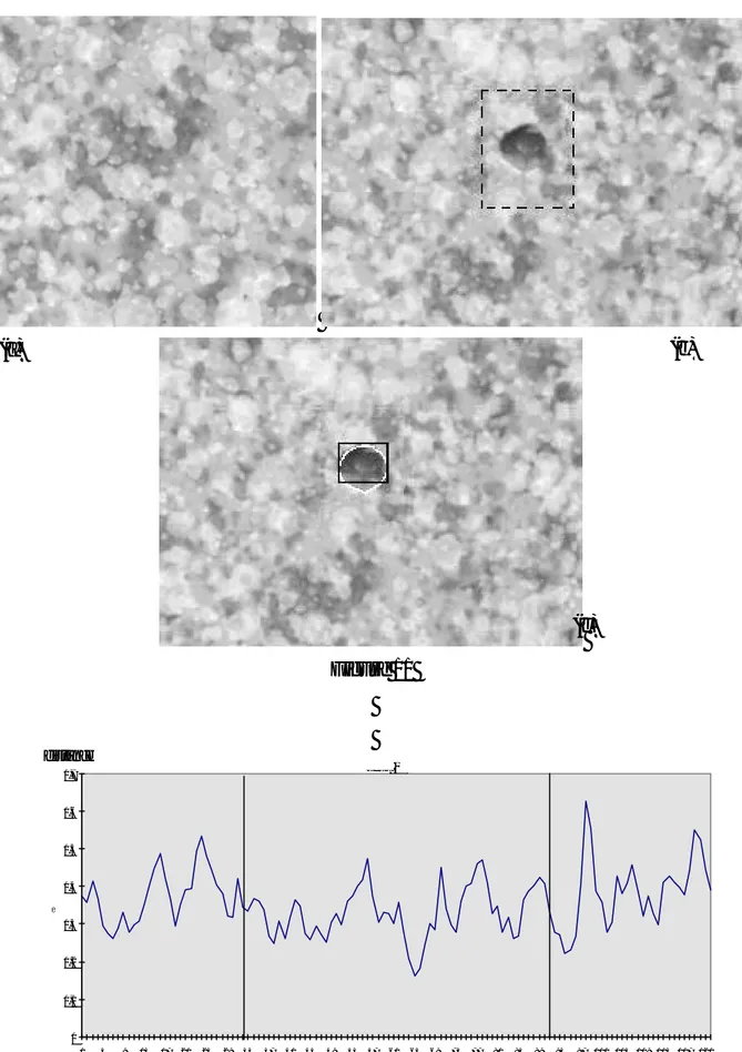
Figs. 7 and subsequent illustrate some examples of natural defect identification. In all the examples shown hereafter, the image was regularly partitioned in blocks of 125x125 pels, to which the texture fault detection algorithm is applied. Furthermore, the size of the window and the number of smoothing iterations were kept fixed M=5 and N=4, respectively, in order to verify the possibility of applying the algorithm to different data sets without fine-tuning the parameter settings. Fig. 7.a presents a detail of a regular ceramic tile, characterized by a pseudo-random enamel glazing, acquired at a resolution of 300 dpi with a uniform illumination system. Fig. 7.b shows a detail of a defective tile, with the region of interest including the flaw marked by a dashed box. Fig. 7.c compares the manual defect segmentation operated by the expert (white line) with the defect bounding automatically extracted by the algorithm (black line). It is possible to observe that only minor discrepancies are present in this case between the two classifications, concentrated in the border of the defective area. As in the synthetic case, the inability of the original max- min approach to solve the problem is made evident by the chart in Fig. 8, which shows the distance of horizontal scan lines of the defective texture from the prototype, based on the parameter “density of extremes”. It is possible to observe that scan lines enclosing the flaw do no t present particular statistical difference as compared to normal samples. On the contrary, Fig. 9 demonstrates that the proposed feature set is able to significantly discriminate among normal and defective areas: in particular, it is to be pointed out that in this case there is not a unique dominant feature (as in the synthetic test), but there is a good complementarity among the various features (e.g., mean value and variance of maxima). Again, the chart in Fig. 10 shows the distances between texture samples and prototype, calculated on the entire feature vector, together with the defect bounding coordinates (horizontal direction) and ideal thresholds (sample coordinates are relative to the region of interest).

In the example of Figs. 11-14, showing the results achieved on a different type of ceramic material, an incomplete detection of the defect is achieved, being the bottom part of the flaw very difficult to characterize in the horizontal direction (as shown by the relevant charts). In Fig. 15, a different defect occurred on the same material of Fig. 11 is identified by the algorithm: in this case, being the defect (a small crack) quite thin and elongated, the algorithm is able to catch only a part of it. This example highlights a limitation of the proposed technique, which provides better results in the presence of defects with isotropous shapes. Finally, in Figs. 16-17 two different defects occurred on a third type of textured tile are exactly detected.

A major problem with natural images lies in the fact that they are usually characterised by less evident defects, with different shapes and dimensions. As a consequence it is often not possible to exactly specify the size and extension of a defect even for a human observer (in particular, the borders are in general ambiguous). Furthermore, the proposed algorithm is not able to perform an

exact segmentation, but just defines the rectangle that bounds the image rows and columns classified as defective. Consequently, to extend the use of a quantitative index of performance to the case of natural images, it was first necessary to ask a human expert to manually segment the defect, and then, to compute the bounding rectangle of the flaw identified by the expert. The performance index is then defined as the percentage difference between the two bounding rectangles (the one defined by the expert and the one computed by the algorithm). The accuracy measured in this case is slightly lower as compared to the synthetic case, with an average error percentage of 4.2%, over a set of 200 images. Again, errors were mainly localised near the borders of defective areas, which usually contain a very low percentage of anomalous pixels (particularly, in round-shaped defect). In the case of natural images, a small percentage of false detection was also recorded, in particular when the window size is set very small in the attempt to identify little defects over very large scale textures: in this case it could happen that the texture statistics within the window are not sufficient to characterise all the possible texture variations within the prototype. Since this can be a limiting factor for algorithm applicability, some studies are being conducted to define a more complex matching, based on the use of multiple prototypes.

6. Conclusions

A new method for the detection of texture fault was proposed, which uses a set of contrast-based features calculated with a separate windowing procedure along x and y directions. The method is an extension of the max- min approach, which exploits the properties of local extremes of the luminance function along one-dimensional scan- lines of a texture to identify anomalous regions. Extensive tests demonstrated the effectiveness of this approach and its appropriateness in the context of automated visual inspection systems. Theoretical estimations of the algorithmic complexity as well as practical ones (through implementation on standard computer platforms as well as on parallel DSP architectures), confirmed the usability of the method in real-time inspection systems.

7. References

[1] Dunn, D., Higgins, W.E., and Wakeley, J., “Texture Segmentation Using 2-D Gabor Elementary Functions”, IEEE Trans. on Pattern Analysis and Machine Intelligence, Vol. 16, No. 2, February 1994, pp. 130- 149.

[2] Weldon, T.P., Higgins, W.E., and Dunn, D.F., “Efficient Gabor Filter Design for Texture Segmentation,” Pattern Recognition, Vol. 29, No. 12, 1996, pp. 2005-2015.

[3] Lambert, G., and Bock, F., “Wavelet Methods for Texture Defect Detection,” IEEE

International Conference on Image Processing (ICIP-97), Vol. 3, 1997, pp.201-204.

[4] Portilla, J., Simoncelli, E.P., “A Parametric Texture Model based on Joint Statistics of Complex Wavelet Coefficients”, International Journal of Computer Vision, vol.40(1), pp. 49-71, Dec 2000

[5] Haralick, R.M., “Statistical and Structural Approaches to Texture,” Proc. IEEE, Vol. 67, 1979, pp. 786-804.

[6] Levy Vehel, J., Mignot, P., and Berroir, J.P., “Multifractals, texture, and image analysis,” in

Proc. IEEE Conf. on Computer Vision and Pattern Recognition, Champaign, IL, June 15-18,

1992, pp. 661-664.

[7] De Natale, F.G.B., “Rank-Order Functions for Image Texture Discrimination,” Int. Journal of

Pattern Recognition and Artificial Intelligence, Vol. 10, No. 8, 1996, pp. 971-984.

[8] Oja, E., Parkkinen, J., and Selkainaho, K., “Detecting Texture Periodicity from the Co-Occurrence Matrix,” Pattern Recognition Letters, Vol. 11, 1990, pp. 43-50.

[9] Valkealahti, K., Oja, E., “Reduced Multidimensional Co-Occurrence Histograms in Texture Classification”, IEEE Trans. on Pattern Analysis and Machine Intelligence, Vol. 20, No. 1, January 1998.

[10] Cross, G.R., Jain, A.K., “Markov Random Field Texture Models”, IEEE Trans. on Pattern Analysis and Machine Intelligence, Vol. 5, No. 1, January 1983, pp. 25-39.

[11] Povlow, B.R., Dunn S.M., “Texture Classification using Noncausal Hidden Markov Models”, IEEE Trans. on Pattern Analysis and Machine intelligence, Vol. 17, No. 10, 1995, pp. 1010-1014.

[12] De Natale, F.G.B., Fioravanti, S., Kittler, J., Marik, R., Mirmedhi, M., and Petrou, M., “Spectral and Rank-Order Approaches to Texture Analysis,” European Transactions on

[13] Latif- Amet, A., Ertuzun, A., and Ercil, A., “An Efficient Method for Texture Defect Detection: Sub-band Domain Co-occurrence Matrices,” Image and Vision Computing, Vol. 18, No. 6-7, 2000, pp. 543-553.

[14] Aras, B., Ertuzun, A., and Ercil, A., “Higher Order Statistics Based Texture Analysis Method for Defect Inspection of Textile Products,” Workshop on Nonlinear Signal and Image

Processing (NSIP-99), Vol. 2, 1999, pp. 858-862.

[15] Meylani, R., Ertuzun, A., and Ercil, A., “Texture Defect Detection Using Adaptive Two-Dimensional Lattice Filter,” IEEE International Conference on Image Processing (ICIP-96), Vol. 3, 1996, pp. 165-168.

[16] Mitchell, O.R., Myers, C.R., and Boyne, W., “A Max-Min Measure for Image Texture Analysis,” IEEE Transactions on Computers, Vol. 26, No. 4, 1977, pp. 408-414.

[17] Du Buf, J.M.H., Kardan, M., Spann, M., “Texture Feature Performance for Image Segmentation,” Pattern Recognition, Vol. 23, No. 4, 1990, pp. 291-309.

FIGURE AND TABLE CAPTIONS

Table I – Time required (in msec) to process a 512×512 pels texture on a Sun Spark Ultra 80 workstation running Sun-Solaris operating system, for various settings of the M, N parameters. Table II - Inter- and intra-set distances of the feature vector clusters achieved by the max-min approach on the textures in Fig. 1.a-b

Figure 1 - (a), (b) two textures taken from the Brodatz album, 512×512 pels; (c) a synthetic pattern obtained by introducing a 100×100 region of texture (b) in texture (a).

Figure 2 - Distance of horizontal scan lines of texture 1.c from the prototype of texture 1.a, with application of the original max-min approach. Vertical lines mark the extraneous area.

Figure 3 - Texture scanning procedure. (a) A horizontal moving window of vertical size 3 is applied to a block. (b) The scanning is repeated in the vertical direction to identify defective pixels.

Figure 4 - Basic elements used for feature vector computation in a sample scan line.

Figure 5 - Distance of texture samples of Fig. 1.c from the prototype, analysed feature by feature (horizontal scanning). Vertical lines mark the defective area

Figure 6 - Distance of texture samples of Fig. 1.c from the prototype after the application of the proposed method (horizontal scanning). Vertical lines mark the defective area, while horizontal line indicates the optimum threshold (perfect identification of the defect).

Figure 7 – Example of texture fault detection on a natural image (ceramic tile). (a) A sample of the regular texture; (b) a sample containing a flaw (dust blotch): the block containing the defect is marked by a dashed line; (c) identification of the defect: by an expert (white) and by the proposed method (black)

Figure 8 - Distance of horizontal scan lines of Fig. 7.b (defective block only) from the prototype extracted from the regular texture of Fig. 7.a, with application of the original max-min approach. Vertical lines mark the horizontal bounds of the flaw.

Figure 9 - Distance of texture samples of Fig. 7.b from the prototype (defective block only), analysed feature by feature (horizontal scanning). Vertical lines mark the defective area

Figure 10 - Distance of texture samples of Fig. 7.b from the prototype after the application of the proposed method (horizontal scanning). Vertical lines mark the defective area, while horizontal line indicates the optimum threshold (set by hand).

Figure 11 – Example of texture fault detection on a natural image (ceramic tile). (a) A sample of the regular texture; (b) a sample containing a flaw (enamel stain): the block containing the defect is marked by a dashed line; (c) identification of the defect: by an expert (white) and by the proposed method (black)

Figure 12 - Distance of horizontal scan lines of Fig. 11.b (defective block only) from the prototype extracted from the regular texture of Fig. 11.a, with application of the original max-min approach. Vertical lines mark the horizontal bounds of the flaw.

Figure 13 - Distance of texture samples of Fig. 11.b from the prototype (defective block only), analysed feature by feature (horizontal scanning). Vertical lines mark the defective area

Figure 14 - Distance of texture samples of Fig. 11.b from the prototype after the application of the proposed method (horizontal scanning). Vertical lines mark the defective area, while horizontal line indicates the optimum threshold (set by hand).

Figure 15 – Detection of another type of flaw on the same textured material of Fig. 11.a. (a) sample containing the flaw (small crack): the block containing the defect is marked by a grey box; (b) identification of the defect: by an expert (white) and by the proposed method (black)

Figure 16 – Detection of another type of flaw on a different material (natural stone). (a) Sample containing a flaw (chipping): the block containing the defect is marked by a grey box; (b) identification of the defect: by an expert (white) and by the proposed method (black)

Figure 17 – Detection of another type of flaw on the same material of Fig. 16.a. (a) sample containing the flaw (bump): the block containing the defect is marked by a grey box; (b) identification of the defect: by an expert (white) and by the proposed method (black)

Table I M N 3 5 7 3 132 223 309 4 185 292 417 5 232 371 512 Table II Maximum intra-set distance

for texture 1.a

Maximum intra-set distance For texture 1.b

Minimum inter-set distance between 1.a e 1.b

0.04419 0.13009 0.19075

(a) (b)

(c)

test 8 0 0,05 0,1 0,15 0,2 0,25 0,3 1 16 31 46 61 76 91 106 121 136 151 166 181 196 211 226 241 256 271 286 301 316 331 346 361 376 391 406 421 436 451 466 481 496 righe distanze Figure 2 INSPECTED WINDOW . . . . . . PIXEL ROW . . . WINDOW HORIZONTAL VERTICAL WINDOW (a) (b) INSPECTED BLOCK INSPECTED INSPECTED BLOCK Figure 3 Figu re 4 0 2 4 6 8 10 12 14 16 1 17 33 49 distanze LOCAL EXTREMES PEAK POWER M1 M3 M2 m1 m2 k GRAYLEVELS SCAN LINE distance Row index distance

Figure 5 test 8 0 1 2 3 4 5 6 7 1 16 31 46 61 76 91 106 121 136 151 166 181 196 211 226 241 256 271 286 301 316 331 346 361 376 391 406 421 436 451 466 481 496 colonne distanze Figure 6 Row index distance (a) (b)

Figure 7 test 1 0 0,05 0,1 0,15 0,2 0,25 0,3 0,35 0,4 0,45 0,5 1 5 9 13 17 21 25 29 33 37 41 45 49 53 57 61 65 69 73 77 81 85 89 93 97 101 105 109 113 117 121 125 righe distanze Figure 8 (c) Row index distance

test 1 0 2 4 6 8 10 12 14 16 18 20 1 5 9 13 17 21 25 29 33 37 41 45 49 53 57 61 65 69 73 77 81 85 89 93 97 101 105 109 113 117 121 125 righe distanze Figure 9 test 1 0 1 2 3 4 5 6 7 1 5 9 13 17 21 25 29 33 37 41 45 49 53 57 61 65 69 73 77 81 85 89 93 97 101 105 109 113 117 121 125 righe distanze Figure 10 density of extrema maxima mean value minima mean value maxima variance minima variance power of peaks power of valleys Row index distance Row index distance

Figure 11 test 2 0 0,1 0,2 0,3 0,4 0,5 0,6 0,7 1 5 9 13 17 21 25 29 33 37 41 45 49 53 57 61 65 69 73 77 81 85 89 93 97 101 105 109 113 117 121 righe distanze Figure 12 (a) (b) (c) Row index distance

test 2 0 2 4 6 8 10 12 14 16 1 5 9 13 17 21 25 29 33 37 41 45 49 53 57 61 65 69 73 77 81 85 89 93 97 101 105 109 113 117 121 righe distanze Figure 13 test 2 0 1 2 3 4 5 6 1 5 9 13 17 21 25 29 33 37 41 45 49 53 57 61 65 69 73 77 81 85 89 93 97 101 105 109 113 117 121 righe distanze Figure 14 Row index distance Row index distance

(a) (b) Figure 15

(a) (b)

(a) (b)