UNIVERSIT `
A DELLA CALABRIA
Facolt`a di Ingegneria
Dipartimento di Elettronica, Informatica e Sistemistica
Dottorato di Ricerca in Ingegneria dei Sistemi ed Informatica
XXIV ciclo
Settore Scientifico Disciplinare ING/INF-05
Tesi di Dottorato
The Generative Aspects of Count Constraints:
Complexity, Languages and Algorithms
Coordinatore
Prof. Luigi Palopoli
Supervisore
Prof. Domenico Sacc`a
Edoardo Serra
Acknowledgments
I owe my deepest gratitude to my mentor Prof. Domenico Sacc`a who, under his direction, has been able to bring out the best of me and give me the right space to take confidence with my capabilities, without never suppress my creativity.
I wish to express my gratitude to Dr. Antonella Guzzo and Dr. Luigi Moccia (Antonella and Luigi) that with their suggestions always help me, proving to be true friends.
Special thanks to Prof. Carlo Zaniolo that during my visit to UCLA (Los Angeles, CA) has been present and under his supervision I spent a productive year.
I wish to thank Prof. Francesco Scarcello (Francesco) whose door are always opened for any theoretical question.
Last but not the least I would like to thank my Dad and my girlfriend Francesca.
Rende,
Contents
1 Introduction. . . 1
1.1 Inverse Frequent set Mining (IFM) . . . 2
1.2 Count constraints and the inverse OLAP problem . . . 6
1.3 Datalog with frequency support goals . . . 9
1.4 Contributions of the thesis . . . 11
1.5 Organization of the thesis . . . 12
2 Inverse Frequent Itemset Mining Problem (IFM). . . 15
2.1 Introduction . . . 15
2.2 Problem Formalization and Complexity Issues . . . 16
2.3 A Level-Wise Solution Approach for IFMS. . . 19
2.3.1 Description of the Algorithm . . . 19
2.3.2 Optimization Issues . . . 21
2.3.3 An Example of computation . . . 22
2.4 Solving the General Case of IFM . . . 23
2.5 Computational Result . . . 24
2.5.1 Test instance . . . 25
2.5.2 Results . . . 25
3 A New Generalization of IFM . . . 29
3.1 Introduction . . . 29
3.2 Problem Formalization . . . 32
3.2.1 The κ-IFMσ0 as an Integer Linear Program . . . 35
3.2.2 The κ-IFMσ0 as a Linear Program . . . 38
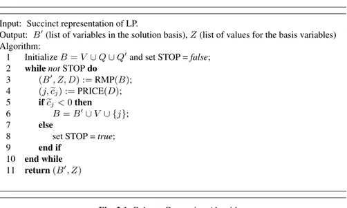
3.3 Column Generation Algorithm to solve LP . . . 39
3.3.1 Column Generation Algorithm . . . 39
3.3.2 Complexity of the Pricing Problem . . . 41
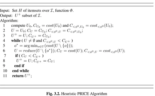
3.3.3 A Heuristic Algorithm for the Pricing Problem . . . 44
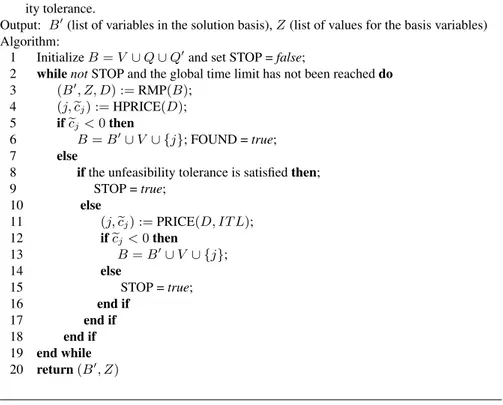
3.3.4 Heuristic Column Generation Algorithm . . . 45
3.4 Computational results . . . 47
3.4.2 Results . . . 50
3.5 Related Works . . . 55
3.5.1 Solving FREQSAT with Heuristic Column Generation Algorithm . . . 57
3.5.2 Comparison with IPF . . . 58
3.6 Applications of IFM . . . 59
4 Count Constraints and the Inverse OLAP Problem . . . 61
4.1 Introduction . . . 61
4.2 Preliminaries and related work . . . 63
4.2.1 From IFM to Inverse OLAP . . . 63
4.2.2 Data Exchange . . . 64
4.3 Count Constraints . . . 64
4.3.1 A Motivating Example . . . 68
4.4 The Inverse OLAP Problem: Definition and Complexity . . . 70
4.4.1 Binary Domain Inverse OLAP . . . 70
4.4.2 Binary Attribute Inverse OLAP . . . 77
4.4.3 Data Complexity of Inverse OLAP . . . 78
4.5 A Step towards Aggregate Data Exchange . . . 79
5 Datalog with frequency support goals. . . 83
5.1 Introduction . . . 83
5.2 Related Work . . . 84
5.3 DatalogF Sby Examples . . . . 85
5.4 Semantics of DatalogF S. . . . 88
5.4.1 Rewriting of DatalogF Sinto Datalog . . . 88
5.4.2 Stratified DatalogF S. . . 89
5.4.3 Recursive DatalogF S . . . 89
5.5 Multi-Occuring Predicates . . . 90
5.6 Implementation & Optimization . . . 93
5.6.1 Differential Fixpoint . . . 93
5.6.2 Magic Sets . . . 95
5.6.3 Avoiding Expansions . . . 96
5.7 Scaling . . . 98
5.8 More Advanced Applications . . . 99
5.8.1 Diffusion Models with DatalogF S . . . 100
5.8.2 Markov Chains with DatalogF S. . . 102
6 Conclusions . . . 107
1
Introduction
Important elements of database models are the integrity constraints . The integrity constraints are used to enhance the expressiveness of data model; In other words the integrity constraints represent properties that the data structure of database must have. If the data satisfy the integrity constraints, such data are said consistent. A typical database model is the relational model, where the data structure is represented as a set of relations and each relation identifies an entity described through a set of attributes. In the relational schema there are more types of constraints as functional dependencies, primary key, foreign key and attributes domain [AHV95]. Consider a classical example of a database of a university where students attend courses and each course is done in a specific quarter of the year. A possible relational schema is the following:
student(idn, name), attend(student, course), course(id, quarter) and we have the following integrity constraints:
• Functional dependencies: Given a relation R, a set of attributes X in R is said to functionally determine another attribute Y in R, X→ Y , if, and only if, each X value is associated with precisely one Y value. A special case of functional de-pendency is the primary key constraint that imposes that each record of a relation is uniquely identified by a specific set of attributes, called key, i.e. in a relation cannot exist two records with the same assignment of values of the key set. In our example course(id, quarter) the key is the underline attribute id that can be express as functional dependency id→ quarter.
• Foreign key constraints: A foreign key imposes that a specific attribute in a rela-tion has values take out of values of a key attribute in an other table, for example with the notations attend( , X)→ ∃Y : course(X, Y ) we indicate that the val-ues of attribute course in relation attend are at most the valval-ues in attribute id in relation course.
• Attribute domain constraints: An attribute domain constraint imposes that all value of a specific attribute in a relation must belong to a specific domain. For
example with the notation course( , Y )→ Y ∈ {fall, winter, spring} we im-poses that each values of the attribute quarter in the relation course must belong to the set{fall, winter, spring}.
• Cardinality constraint: A cardinality constraint is a special constraints that im-poses that the cardinality of a specific projection over a relation, belongs to a particular range of values. We recall that the projection operation extracts only the specified attributes from a tuple or set of tuples [AHV95]. In the example we have that every course must have at least 20 students and at most 25.
Common problems dealing with integrity constraints are: data consistency check-ing and constraints consistency checkcheck-ing. Since the integrity constraints imply that the data in the database must have a particular structure, the first problem consists in verifying if the data in the database satisfy the given constraints (this phase is also called check phase). Typically data consistency check is done after a change (update or insert) of the data, and the validation depends on the result of the check phase. When there is a lot of constraints (especially in the context of ontology), an other interesting problem consist in verifying if there exists at least a data structure that satisfy them, in such case the constraints are said consistent (constraints consistency checking). Actually, current literature focused on the decisional version of both two problems, while the generation of data has not been enough investigated. Conversely, we consider the constraints discussed above, from a different point of view, that is by investigating on the generative aspect, i.e. the way to materialize the data that sat-isfy them. Moreover, we focus on a special type of constraint over aggregate value, called count constraint, which is described by two elements: a description of the set in which the count aggregate is applied and a numeric interval in which the value of the count aggregate must belong. We will briefly show in the Section 1.2 how our count constraints are able to express all previous integrity constraints.
We consider the generative aspect of count constraint in the following three con-texts:
1. Transaction database and support constraints (Section 1.1); 2. Relational database and count constraints (Section 1.2);
3. Deductive database: datalog with frequency support goals (Section 1.3).
1.1 Inverse Frequent set Mining (IFM)
Transaction databases are databases where each tuple, called itemset (or transac-tion), is defined as a subset of a fixed set of itemsI (e.g. in market data, a transaction corresponds to one purchase event and each item is a salable product). Given an item-set J and a transaction database, two measure are defined: (i) number of duplicates, i.e. the number of times that the itemset appears in the transaction database, and (ii) support, i.e. the number of itemsets in the transaction database that contain the spec-ified itemset. An example of transaction database over the itemsI = {a, b, c, d} is the following:
1.1 Inverse Frequent set Mining (IFM) 3 transaction NDUP {a, b, c} 8 {a, b, d} 14 {a, b} 4 {d} 2
where the field transaction represents the itemsets and NDUP are its numbers of duplicates for the itemsets. Over such database, given an itemset subset of{a, b, c, d} we can compute its support; for example, the support of{a, b} is equal to 8+14+4 = 26 because{a, b} is contained in {a, b, c}, {a, b, d} and {a, b}.
The Inverse Frequent set Mining problem (IFM) [Mie03] is the following. Given a set S of frequent itemsets subset ofI and a specified range of support for each itemset in S, construct a transaction database D (if any exist) that satisfies a set of support constraints over S. A support constraint is a triple composed by an itemset I and two non negative integers σminand σmaxthat represents the extremes of range
[σmin, σmax] . Such support constraint is satisfied in a database D if the support of
the itemset I belongs to [σmin, σmax]. It is important to notice that, since the support
of an itemset is the number of transactions that contain this itemset, then a support constraints can be seen as a specialization of count constraint. Its major applications concern privacy preserving and generator for benchmarking data.
For example, consider the following instance of IFM over a set of items{a, b, c, d}: I σminσmax
{a, b, c} 8 10 {a, d} 10 14 {b, d} 18 20
{d} 20 40
where the field I represents the itemset and [σmin, σmax] is the ranges of its
support. The following two databases satisfy this constraints: transaction NDUP {a, b, c} 8 {a, b, d} 14 {b, d} 4 {d} 2 transaction NDUP {a, b, c, d} 6 {a, b, c} 2 {a, b, d} 8 {b, d} 6
Normally, the itemsets provided in S are only the frequent ones, i.e. the itemsets whose support is greater or equal than a fixed threshold. However, with classical IFM formulation this assumption is not holds. In fact IFM formulation does not impose that each itemset not in S must be infrequent i.e. with a support below than the frequency threshold. As an example, we can see in the previous two databases, that the support of{a, b} is 22 in the first database and 16 in the second. If we compare the support of{a, b} with respect to the support of other itemset in S we cannot say that{a, b} is infrequent. Therefore the itemset {a, b} results frequent even if it is not specified. We consider this aspect as an anomaly of the formulation.
To solve this anomaly we initially define a new version of IFM, called IFMS.
Such formulation, under the assumption that each itemset not in S must be infre-quent (not significant), imposes that each itemset not in S has support equal to zero or equivalently the number of duplicates is zero. We prove that this subproblem is NP-complete, and provide an heuristic algorithm that always satisfies the maximum support constraints, but that treats minimum support constraints as soft ones that are enforced as much as possible. In fact, a thorough experimentation evidences that minimum support constraints are hardly violated in practice, and that such negligible degradation in accuracy is compensated by very good scaling performances.
Despite the IFMSsolves this anomaly, the assumption that each itemset not in S
must have a support equal to zero, can be restrictive. Consider the following instance over itemsI = {a, b, c}.
I σmin σmax
{a, c} 4 4
{b, c} 3 3
{c} 5 5
Since the number of duplicates or the support of itemsets not in S must be equal to zero, then the itemset in D can only be the itemset in S. Thus, there is not solution to the IFMSproblem in fact the database that satisfies the previous constraints must
have the following structure:
transaction NDUP
{a, c} ?
{b, c} ?
{c} ?
It is easy to see that, if we satisfy the first two constraints over itemsets{a, c} and {b, c}, automatically the constraint over itemset {c} is violated because its support is equal to 4 + 3 = 7.
If we admit that can exist in the database other itemsets not defined in S but with limited support (in this case less or equal 2), then it is possible generate a database that satisfies the above constraints. Such database is the following:
transaction NDUP {a, b, c} 2
{a, c} 2
{b, c} 1
It is important to notice that the support of{a, b, c} is less than of the one of other itemset in S, therefore it can be considered infrequent.
To tackle this problem we propose a pregeneration method. The pregeneration method consists to generate a new instance of IFMSover an extended set of itemsets
S∪ S+where S+is a the set of new itemsets different from S. The pregeneration method heuristically builds by using itemsets in S, a limited number of itemsets not in S that puts in S+. In the new instance of of IFMS is imposed that the support of
1.1 Inverse Frequent set Mining (IFM) 5 At this point it is important to show that not all itemsets not in S can be con-strained. Consider, in fact, the following instance over a set of items{a, b, c}:
I σmin σmax
{a, c} 4 4
{c} 5 5
If we impose that the threshold of new itemsets σ0is equal to 2, then the itemset{a}, not contained in S, must have a support less or equal to 2, and therefore the itemset {a, c} cannot have a support equal to 4 but only 2. For this reason, we constraint only the itemsets not in S such that does not exist an itemset in S that contains them, such set is called S0
S0={I ∈ UI\ S |@I0∈ S : I ⊂ I0}
where UIis the set of all itemsets contained inI. We think that the information about of itemsets in S are more accurate w.r.t the succinct information given by the thresh-old support for the itemsets not in S. In Chapter 2 are reported the IFMS
formaliza-tion, the IFMS heuristic, the pregeneration method, and their relative experimental
results.
Nevertheless the experimental results of previous methods are satisfactory, the pregeneration of a limited set of itemset is not always sufficient, because it is difficult to establish what are the itemsets that can improve the satisfying of the constraints in S.
An alternative approach that significantly improve the previous results consists in a generation of itemsets not in S of the type step by step, i.e. starting with a fixed set of itemsets, solve the problem with such set and after try to find a new itemset that can improve the current solution. Such process continues until the current solution satisfies each constraint or does not exist an other itemset that improves the solution. The big problem in such approach is that we must always guaranty that the sup-port of itemsets in S0 is less or equal than a fixed threshold. For this reason, we provide a new formulation called IFMσ0, that imposes that each itemset not in S has
a support less or equal than a fixed threshold σ0. We will show that this problem is NEXP-complete and such complexity is caused by imposing that each itemset not in S has a support less or equal to σ0. In fact to verify that a database satisfies all the constraints, we must compute for each itemset, its support and the number of each itemset in S0can be exponential in the size ofI.
Even if the monotonicity property of the support allows to verify only the support of the minimal itemsets in S0, i.e. the set BS0 defined as follow:
BS0 ={I ∈ S0| 6 ∃J ∈ S0: J⊂ I}
the cardinality of BS0 can be exponential in the size of S. In fact, consider the
fol-lowing set of itemsets S over the itemsI = {a0, a1, b0, b1, c0, c1}: S
{b0, b1, c0, c1} {a0, a1, c0, c1} {a0, a1, b0, b1}
the set BS0is : BS0 {a0, b0, c0}, {a0, b0, c1} {a0, b1, c0}, {a0, b1, c1} {a1, b0, c0}, {a1, b0, c1} {a1, b1, c0}, {a1, b1, c1}
As it is possible to see, the cardinality of BS0 is equal to 23, where 3 is the number
of the itemsets in S. In same way, it is possible to produce exponential examples (|BS0| = 2n) with n itemsets in S and 2∗ n items.
Because BS0can still be exponential in the size of S, we individuate a parameter
k relative to the number of items. If this parameter is bounded, then also the cardinal-ity of BS0 is bounded. Such parameter allows to define a parametrization of IFMσ0,
called κ-IFMσ0, that can be reduced to the original IFM problem, thus they have the
same complexity: NP-hard and PSPACE.
Moreover we will show that the IFMσ0 can be formulated as an integer linear
problem with huge number of variables and constraints, in general both exponential in the size of the input. At the same time it will showed that the parametric versions can be solved as an integer linear problem only with a huge number of variables.
In order to concretely solve κ-IFMσ0, we relax the integer constraints over the
number of duplicates and use the column generation method [DT03, DDS05] that is an efficient way to solve particular linear problem with a huge number of variables.
In order to use the column generation method, it is necessary solve its specific pricing problem. In our context the pricing problem is NP-complete and we solve this in exact way by an efficient integer linear formulation and a heuristic way by using a greedy dept-first algorithm.
The experimental results prove that our new approach is efficient and effective and the relaxed integer approximation does not compromise the quality of results. Moreover, despite the IFMσ0 presents a strong complexity, the real life instances
considered, present a very small value of the k parameter, and, therefore, they are tractable with our approach. The problem IFMσ0 with its parametrization κ-IFMσ0
and column generation methods are discuss Chapter 3.
1.2 Count constraints and the inverse OLAP problem
In the context of relational databases, we propose integrity constraints based on the first order predicate calculus. Such a constraint is represented by a rule of following form:
∀X ( α → βmin≤ #({ Y : γ }) ≤ βmax).
The head of such rule represents an integer interval where the value of count aggre-gate #({Y : γ }) must belong, and the body α is a conjunction of atoms. For brevity, in this section we explain part of the syntax and semantics of our count constraints by some examples.
1.2 Count constraints and the inverse OLAP problem 7 Consider the initial examples of integrity constraints over the schema:
student(idn, name), attend(student, course), course(id, quarter) We can rewrite the previous constraints by using our count constraints: • the functional dependency (the primary key) can be express as
∀ID ( Did(ID)→ 0 ≤ #({Q : course(ID, Q)}) ≤ 1)
where Did is the domain of attribute id in the relation course. Such constraint
can be intuitively read as: for the each value of domain Didthere is at most one
tuple with such a value of id. • the foreign key can be expressed as
L = #({ID : attend( , ID)}) → L≤ #({ID : attend( , ID), course(ID, )}) ≤ L
Such constraint can be intuitively read as: let L the number of id values of the relation attend then the number of id of relation attend that are also present in the id values of the relation course is equal to L .
• in the same way of foreign key we can model the domain attribute constraint: L = #({Y : course( , Y )}) → L≤ #({Y : course( , Y ), Y ∈ {fall, winter, spring}}) ≤ L • The cardinality constraint can be express as
∀C ( course(C, ) → 20 ≤ #({S : attend(S, C)}) ≤ 25)
Such constraint can be intuitively read as: for each course C the number of stu-dents that attend the course C is between 20 and 25.
Actually, our language is more complex and provides the using of sets definitions. Consider the relational schema formed by only one relation trans(tid, item) with domains Dtidand Ditem. Such relation schema plus count constraints can be used to
express the problem of Inverse Frequent Itemset over transaction Databases defined in Section 1.1. In fact the following transaction database can be transformed in an instance of the relation trans:
transaction NDUP {a, c} 2 {b, c} 1 ⇒ trans id tid 1 a 1 c 2 a 2 c 3 b 3 c
where Dtid = {1, 2, 3} and Ditem = {a, b, c}. Therefore, if we want to describe
some constraints over the support of itemsets we can use our count constraints with the set definition. For example, if we want to say that the support of itemset{a, b, c} is between 4 and 6 we can use the following count constraint:
I ={a, b, c} → 4 ≤ #({T ID : I ⊆ {IT EM : trans(T ID, IT EM)}}) ≤ 6 This constraint can be read in the following way: let I be the set{a, b, c} then the number of tid (transactions) s.t. I is a subset of the set of items belonging to tid is between 4 and 6.
In the following, similarly to the problem of Inverse Frequent set Mining, we define the inverse OLAP problem where, instead of find a transaction database that satisfies a specific set of constraints over the support of the itemsets, we want to find a relational database that satisfies a set of our count constraints.
We focus on a relation schema typical in the world of OLAP [CD97, LL03, Han05], i.e. the star schema (see Fiugure 1.1) that consists of one fact table refer-encing any number of dimension tables.
Fig. 1.1.Star schema
The fact table represents the relation where the values to aggregate are contained. In our case, we consider only count aggregates, and then the fact table is only a relation R(A1, . . . , An) with n > 0, where the domains D1, . . . , Dn are specified.
The dimension tables are configured as hierarchy domains, i.e. binary relation linked to some attribute in R. Thus, the inverse OLAP problem is the following: given a set of of domains D1, . . . , Dnwith possibly a fixed additional number of hierarchy
domains and a set of count constraints, decide whether there exists (or to find) a relational table R(A1, . . . , An) that satisfies the count constraints.
Similarly to the query problems in databases it is possible to consider for this problem several type of complexity [Var82]: data complexity (in input only the do-mains), program complexity (in input only count constraints) and combined com-plexity (in input domains and count constraints). We prove that inverse OLAP is NEXP-complete under data, program and combined complexity. Note that, since
1.3 Datalog with frequency support goals 9 our count constraints are very expressive (see the previous integrity constraints ex-pressed with our count constraints), consider only star schema is not a limitation.
In Chapter 4 are describe in a extensive way the syntax and semantics of count constraints, the inverse OLAP problem, and its special cases with complexity anal-ysis; in addition, in the last part of the chapter, some examples showing that our framework is step toward the data exchange problem with count constraints are de-scribed. We recall that this is the problem of migrating a data instance from a source schema to a target schema such that the materialized data on the target schema satis-fies the integrity constraints specified by it.
We belive that the strict connection between inverse OLAP and IFM problem, can help us to export the efficient approach used for IFM in the case of inverse OLAP.
1.3 Datalog with frequency support goals
Similarly to the language of count constraints above presented, we introduce a simple extension of Datalog [Hel10, dMMAG, HGL11], called DatalogF S, that enables us to query and reason about the number of distinct occurrences satisfying given goals, or conjunction of goals, called Frequency Support goal (or FS-goal), in rules. The form of FS-goal is the following:
Kj : [exprj(Xj, Yj)]
where Kj is the counting variable and exprj(Xj, Y j) is a conjunction of positive atoms. Such count atom is satisfied, intuitively, if there exist Kjdifferent satisfying
ground instances of exprj(Xj, Y j). In the following, we show a simple program in DatalogF Sthat computes the persons that will come to a particular event.
willcome(X)← sure(X).
willcome(Y)← 3:[friend(Y, X), willcome(X)].
The last rule is based on the assumption that a person will come to an event if at least three friends will come to this event. In fact, as it is possible to see by the FS-goal 3 : [friend(Y, X), willcome(X)], in the program we derive the predicate wilcome(y) if y has at least three different friends x1, x2, x3 ( friend(y, x1), friend(y, x2) and friend(y, x3)) such that x1, x2, x3 will come to the event ( wilcome(x1), wilcome(x2) and wilcome(x3)).
In the previous program the counting variable Kj is fixed to the value 3. How-ever, in a general program Kj is not fixed and can be present in other predicates in the body or directly present in head of the a rule, as in the last rule of the following example that computes the number of friends of a person.
friend(x0, x1) friend(x0, x2) friend(x0, x3)
In this case, the facts nFriend(x1, 1), nFriend(x1, 2) and nFriend(x1, 3) are de-rived. Actually, we are only interested in the fact nFriend(x1, 3) that contains the maximum value of the counting variable K. For this reason, we introduce the m-predicates (multiplicity m-predicates) that, instead of storing a fact for each value as-sumed by K , it directly stores the multiplicity fact with the maximum value of K. In this case the last rule of the previous program is rewritten by using an m-predicates as follows:
nFriend(X) : K← K:[friend(X, Y)].
and the derived facts are only nFriend(x1) : 3. It is important to notice that we do not change the semantics but only the way of computing. More specifically, the fact nFriend(x1) : 3 is a compact way to represents the three facts nFriend(x1, 1), nFriend(x1, 2) and nFriend(x1, 3) i.e. if we know nFriend(x1) : 3 then we also know nFriend(x1) : 2 and nFriend(x1) : 1.
Consider now the following program, where, given a complex object formed by a fixed number of subpart (a subpart can be a basic object or an other complex object), it able to compute the number of elementary part of the complex object. Let basic(part) be facts that describe the basic part and assbl(part, sub, qty) be the facts that describe the number (qty) of sub-part (sub) that are present in a complex object (part), the program is the following:
cassb(Part, Sub) : Qty ← assbl(Part, Sub, Qty).
cbasic(Pno) : 1← basic(Pno).
cbasic(Part) : K← K : [cassb(Part, Sub) : K1, cbasic(Sub) : K2]. In this example we can see two m-predicates cassb and cbasic were the respective multiplicity variable are Qty (first rule) and K (second rule). The first rule transforms the quantity information Qty stored in assbl(Part, Sub, Qty), in a multiplicity of predicate cassb, e.g. if there exists the fact assbl(p1, p2, 2) the first rule derives two multiplicity facts cassb(p1, p2) : 1 and cassb(p1, p2) : 2, and in the interpreta-tion are stored only the fact cassb(p1, p2) : 2. The last two rules with m-predicate cbasic are used to compute the number of basic elements of a particular complex object. In the last rule the FS-goal K : [cassb(Part, Sub) : K1, cbasic(Sub) : K2] computes the number of basic element. Consider the following example wsere we have two basic part s cbasic(p1) : 1 and cbasic(p2) : 1, and the complex object p is formed by two basic object of p1 and one basic object of p2 (cassb(p, p1) : 2 and cassb(p, p2) : 1). Therefore, we have the following three ground instance that satisfy cassb(Part, Sub) : K1, cbasic(Sub) : K2 conjunction:
cassb(p, p1) : 2, cbasic(p1) : 1 cassb(p, p1) : 1, cbasic(p1) : 1 cassb(p, p2) : 1, cbasic(p2) : 1 The derived result is cbasic(p1) : 3.
1.4 Contributions of the thesis 11 Moreover, as it possible to see in the last rule of the previous example, we can give recursive definitions that use the FS-goal, this because the FS-goal is monotone. We prove, by an elegant rewriting of the FS-goal by using lists, that the immediate consequence operator of DatalogF Sis monotone. We show how this simple extension
is able to express more queries in the context of social networks, and work with Markow chains. More details are given in Chapter 5.
1.4 Contributions of the thesis
In this section we summarized our contributions in each of the contexts above dis-cussed.
Inverse Frequent set Mining
• We define IFMS problem where the itemset not in S has support equal to zero,
prove that its complexity is NP-complete and provides an heuristic level-wise algorithm for its resolutions.
• We provide a pregeneration method to extract new itemsets not contained in S. • We give some experimental results showing that the heuristics algorithm for
IFMSproblem combined with the pregeneration is a good approach to IFM
prob-lem.
• We define the IFMσ0 problem where the itemset not directly specified in input instance are constrained to be infrequent i.e. they have a support less or equal to a specified unique threshold. Its complexity is NEXP-complete.
• We find a parameter K relatives to the number of items. Such parameter allows to define a parametrization of IFMσ0, called κ-IFMσ0, that can be reduced to
origi-nal IF M problem, thus they have the same complexity NP-hard and PSPACE. • We show that the IFMσ0 can be formulated as an integer linear problem with
huge number of variables and constraints, in general both exponential in the size of the input. At the same time we show that the parametric versions can be solve as an integer linear problem only with huge number of variable.
• In order to concretely solve κ-IFMσ0 we relax the integer constraints over the
number of duplicates and used the column generation method that is an efficient way to solve particular linear problem with an huge number of variable.
• Since to use the column generation method it is necessary solve its specific pric-ing problem, we study its complexity (NP-complete) and proposed a formulation of ILP and a polynomial heuristic.
• We show by experimental results that the approach for IFMσ0 is efficient and
effective and the relaxed integer approximation did not compromise the quality of results. Moreover, despite the problem presents a strong complexity, the real life instances considered, present a very small value of k parameter, and therefore they are tractable with our approach.
Count constraint and inverse OLAP problem
• We provide a new language to define count constraints in relational schema whose special cases are well known relational integrity constraints.
• Similarly to IFM problem we define the inverse OLAP problem: given a set of at-tribute domains and a set of count constraints verify if there exists (and eventually find) a relational database over the given domains that satisfies the constraints. • We prove that inverse OLAP is NEXP-complete under data-complexity,
program-complexity and combined program-complexity.
• We individuate many significative sub-problems of inverse OLAP.
• We show how the Inverse OLAP problem can be a step toward data exchange with aggregate constraints.
Datalog with frequency support goals
• We provide an extension of Datalog, called DatalogF S, that enables us to query
and reason about the number of distinct occurrences satisfying given goals, or conjunction of goals, in rules.
• We prove by an elegant rewriting of frequency support goal that the immediate consequence operator of DatalogF Sis monotone and continuos. This allow as to
also write aggregate recursi ve query in our language.
• We extend the traditional techniques for classical Datalog programs optimiza-tions as differential fixpoint and magic set to DatalogF S.
• We introduce an optimization technique that compute in efficient way DatalogF S
program with the count variable is in the head.
• We show as DatalogF Sextends the application range to support page-rank and
social-network queries
1.5 Organization of the thesis
The thesis is organized as follows:
In Chapter 2 we describe the IFMS problem with its complexity analysis and
a heuristic solution. Moreover we provide the pregeneration methods and show the experimental results.
In Chapter 3 we give a formalization of IFMσ0 problem, its parametrization
κ-IFMσ0and the integer linear programming formulation of both. Moreover we pro-vide an approximation of κ-IFMσ0 based on the relaxation of integer constraints. In
addition we proposed a resolution method based on the column generation approach and provide its relative pricing problem. In this Chapter, we also study the com-plexity of the pricing problem, its integer linear programming formulation and an heuristic algorithm as its solution. Finally we show the experimental results.
In Chapter 4 we provide an extensive language to define count constraints. Next, we give the formulation of inverse OLAP and we analyzed its complexity in depth. Moreover, several examples are used to show the applicability of our results, and
1.5 Organization of the thesis 13 in particular we describe how inverse OLAP is a step toward data exchange with aggregates .
In Chapter 5 we define an extension of Datalog with frequency support goals, called DatalogF S. We provide the syntax and semantic of the new language. Then,
many applications about page rank and social networks queries are formulated with our language.
2
Inverse Frequent Itemset Mining Problem (IFM)
The Inverse Frequent itemset Mining (IFM) is the problem of computing a transac-tion database D satisfying specified support constraints on a given set S of itemsets, that are typically the frequent ones. Earlier studies focused on investigating computa-tional and approximability properties of this problem, that is NP-hard. In particular, a interesting subproblem formulation is considered where the transaction (itemset) in D are the only itemset in S and minimum and maximum support constraints can be defined on each itemset. Within this setting, an algorithm is proposed that al-ways satisfies the maximum support constraints, but which treats minimum support constraints as soft ones that are enforced as long as it possible. In fact, a thorough experimentation evidences that minimum support constraints are hardly violated in practice, and that such negligible degradation in accuracy (which is unavoidable due to the theoretical intractability of the problem) is compensated by very good scaling performances.
2.1 Introduction
The inverse frequent set mining problem is the problem of computing a database on which a given collection of itemsets must be “frequent” [Mie03]. This prob-lem attracted much attention in the recent years, due to its applications in privacy preserving contexts [WW05, WWWL05] and in defining generators for benchmark data [RMZ03]. In particular, earlier studies mainly focused on investigating its com-putational properties, by charting a precise picture of the conditions under which it becomes intractable (see, e.g., [Cal04, Cal08, Mie03]), and by observing that in its general formulation it is NP-hard even if one looks for approximate solu-tions [WW05].
In this chapter, the inverse frequent set mining problem is reconsidered from a pragmatic point of view instead. Indeed, we concentrate on defining heuristic approaches that are able to efficiently and efficaciously solve the problem in real-world scenarios. In particular, we consider the original formulation of the problem in [Mie03], where the “frequency” of any itemset in the database is measured in terms
of its support, i.e., as the number of the transactions in which it occurs. Note that other approaches to the inverse frequent set mining problem (e.g., [Cal04, Cal08]) considered the actual frequency, i.e., the support divided by the total number of trans-actions; however, as discussed in [Mie03], supports convey more information than frequencies and hence the perspective of [Mie03] is adopted here. In fact, while keeping this perspective, we investigate a more general setting obtained by relax-ing the simplifyrelax-ing assumption in [Mie03] that the size of the output database must be known beforehand, and by furthermore considering a minimum and a maximum support constraint (over each itemset required to occur in the database) in place of a single support value.
2.2 Problem Formalization and Complexity Issues
LetI = {o1, . . . , on} be a finite domain of elements, also called items. Any
sub-set I ⊆ I is called an itemset over I. The universe of itemsets UI is the set of all non-empty itemsets overI. A database D over I is bag of itemsets, each one usu-ally called transaction. The number of transactions inD is denoted by |D|. Given a databaseD over I, for each itemset I over I (I ∈ UI), the support of I, denoted by σD(I), is the number of transactions containing I, and the number of duplicates of I, denoted by δD(I), is the the number of transactions equal to I. We say that I is a frequent itemset inD w.r.t. a given support threshold s if σD(I) ≥ s. Observe that supports are also represented in the literature as a percentage w.r.t. the dimension of D, i.e. by σD(I)/|D|. Finding all the frequent itemsets in D is the well-known
fre-quent itemset mining problem. The anti-monotonocity property holds for supports: given two itemsets I and J with I ⊂ J, σD(J )≤ σD(I).
We denote the set of natural numbers byN0that will be used for bound. We also introduce the symbol∞ to denote an unlimited bound and define ˜N0asN0∪ {∞} — we therefore assume that for each i∈ N0, i < ∞ holds. Finally, we denote the set of pairs{(a, b) : a ∈ N0, b∈ ˜N0, a≤ b} by ˜N2. In the chapter, we consider the inverse frequent itemset mining problem: Given a set S of itemset, finding a database in which each element of S is frequent. This is formalized below.
Definition 2.1 (IFM Problem). Let:
1. S be a given set of itemsets over the items inI
2. Γσ ={(I, σminI , σmaxI ) : I ∈ S, (σImin, σImax)∈ N2} be a given set of triples
assigning a minimum and the maximum support to each itemset in S
Then, the Inverse Frequent Itemset Mining Problem onI, S and Γσ(short: IFM(I, S, Γσ))
consists of finding a databaseD over I such that the following condition hold (or eventually state that there is no such a database):
∀I ∈ S : σI
min ≤ σD(I)≤ σ I
max (2.1)
2.2 Problem Formalization and Complexity Issues 17 It is worthwhile noticing that the inverse frequent mining problem was mainly formulated and analyzed in the literature within contexts where the frequency of an itemset (i.e. its support σD divided by the total number of transactions in D) is considered in place of the support in the problem formulation. When using this per-spective, IFM is generally referred to as the FREQSAT problem, and various com-plexity results are known for it. For instance, it is well-known that FREQSAT is NP-complete (even if the size of each transaction is bounded by some given input parameter or if σmin= σmax) andPP-hard—hence, intrinsically more complex—if
the maximal number of duplicates of any transaction is bounded by some parameter [Cal04].
Considering the support of the itemsets rather than their frequency received con-siderably less attention instead. In particular, in [Mie03], a slight variation of IFM was studied where the size|D| of the output database D is fixed beforehand (short: IFM|D|). This variation was observed to be NP-hard, even if σmin = σmax.
How-ever, the complexity of the main problem IFM (i.e., in absence of such an additional constraint on the size ofD) was not derived in earlier literature. Our first contribution is precisely to complete the picture of the complexity issues arising with the decision version of the inverse frequent mining problem. Indeed, we shall evidence that IFM is computationally intractable too, thereby calling for (heuristic) solution approaches that are efficient in actual scenarios.
Proposition 2.2. IFMis NP-hard, also when σI
min= σmaxI for all I in S.
Note that there are several sources of intractability in the formulation of IFM. The first one is that the “structure” of the various transactions to be inserted intoD is not known beforehand. Therefore, when building such database we are uncertain on which kinds of transaction to exploit. Towards devising heuristic approaches for IFM, a natural idea is then to consider a simplification of IFM where for each itemset J in UI\S not frequently, σD(J ) = 0 or δD(J ) = 0, i.e. all the possible transactions are taken from the set S of itemsets provided in input.
Definition 2.3 (IFMSProblem). Let:
1. S be a given set of itemsets over the items inI
2. Γσ ={(I, σminI , σmaxI ) : I ∈ S, (σImin, σImax)∈ N2} be a given set of triples
assigning a minimum and the maximum support to each itemset in S
Then, the IFMSProblem onI, S and Γσ(short: IFMS(I, S, Γσ)) consists of finding
a databaseD over I such that the following two conditions hold (or eventually state that there is no such a database):
∀I ∈ S : σI min ≤ σD(I)≤ σ I max ∀J ∈ UI\ S : δD(J ) = 0 2 Rather surprisingly, we next show that even IFMSis intractable in general.
Theorem 1 IFMSis NP-complete in general whereas it is feasible in polynomial time if σImin= σmaxI for all I in S.
Proof.
Let us first consider the general case. To prove that IFMS is in NP, we observe
that the size of the output databaseD is certainly bounded by |S| and by the largest support required in the specification. Hence, in polynomial time a non-deterministic Turing machine may first guess such database (basically, the support for each itemset I in S) and then verify whether it satisfies the constraints σi
minand σmaxi , by simply
computing the support σD(Ii) onD.
We now prove that IFMS is NP-hard by exhibiting a reduction from the graph
3-colorability problem of deciding whether, given a graph G = (V, E), there is a 3-coloring c : V → {r, g, b} such that c(i) 6= c(j) for each pair of edges (i, j) ∈ E.
Based on the input graph G = (V, E), we construct an instance of the IFMS(I, ΓS)
problem such that: the setI of items is {r, g, b, l1, l2, l3}∪{vx|x ∈ V }∪{ez,y|(z, y) ∈
E}, where conceptually the item r, g, b are the colors in G, l1, l2, l3are labels imple-menting an encoding of the three colors, vxis an item for each node in G and ez,y
is an item for each edge in G. The encoding of colors by label is such that any two colors share exactly one label; in the proof we shall use the encoding r = {l1, l2}, g ={l1, l3} and b = {l2, l3}.
The set ΓScontains two groups of constraints:
Group (I): these constraints are repeated for each node x ∈ V and enforces that x must be colored with exactly one color. There are 7 itemsets associated to x organized on 3 levels:
• 3 itemsets at the highest level 2: there is an itemset for each possible color c for x, containing the items corresponding to the node x, to all the arcs leaving x, to the color c and to the encoding of the color — the support for such itemsets can be either 0 or 1;
• 3 itemsets at level 1: there is an itemset for each of the 3 encoding labels, contain-ing the item correspondcontain-ing to the label and the item correspondcontain-ing to the node x – the support must be exactly 1;
• 1 itemset at level 0 containing the item corresponding to the node x – its support must be exactly 2;
We explicit the constraints below:
• (Ix,r, 0, 1), (Ix,g, 0, 1), (bx,r, 0, 1), where Ix,r = {vx, r, l1, l2} ∪ I, Ix,g =
{vx, g, l1, l3} ∪I, Ix,b={vx, b, l2, l3} ∪ I, and I = {ex,y|(x, y) ∈ E};
• ({l1, vx}, 1, 1), ({l2, vx}, 1, 1) and ({l3, vx}, 1, 1);
• ({vx}, 2, 2).
Because of the support constraints for the itemsets at level 1,{l1, vx} cannot occur as
transaction in D as it inherits support from those itemsets; in addition, as the support of{l1, vx} is 2 and there are 3 itemsets at level 1 with obligatory support 1, exactly
one of the itemsets at level 1 must occur as transaction, whereas the other two inherit support from a same itemset at level 2. It turns out that exactly one itemset at level 2
2.3 A Level-Wise Solution Approach for IFMS 19
can occur as transaction whereas all others must have support 0 - the itemset selected as transaction will then fix the unique color for the node x.
Group (II): these constraints are repeated for each edge (x, y)∈ E and enforce that two end nodes of the edge have different color. There are 3 itemsets, one for each possible color; the constraints are:
• ({r, ez,y}, 0, 1), ({g, ez,y}, 0, 1), ({b, ez,y}, 0, 1).
The above itemsets inherit support from two itemsets at level 2: one for x and the other for y. The constraints of Group (II) enforces that the two itemsets at level 2 cannot be of the same color, thus any two adjacent nodes cannot share the same color. It follows that the existence of a solution to IFMS witnesses the fact that the
graph G admits a 3-coloring; on the other hand, if IFMS has no solution then the
graph cannot be 3-colored. Hence, IFMSis NP-hard in general.
To conclude the proof, we observe that in the special case where σImin = σImax
holds for all itemsets I in S, one may encode the solutions of IFMS in terms of a
system of linear equations over|S| variables and constraints. The result then follows, since it is well-known that deciding whether a system of linear equations admits a solution is feasible in polynomial time — note that in this case an integer number
solution is also required. 2
2.3 A Level-Wise Solution Approach for IFM
SIn order to devise an efficient and effective algorithm for IFM, we find convenient to firstly tackle the special case where the output database must be constructed by using as transactions the input itemsets only (cf. IFMS problem), and then to build
the general algorithm for IFM on top of the solution approach for IFMS.
In fact, given that it is not possible to efficiently enforce both the minimum and the maximum support on each itemset in S (cf. Theorem 1), we shall propose in this section an approach to face IFMS which takes care for all I in S of the constraint
over σmaxI only, while treating the constraint over σImaxas a soft constraint that must be satisfied as long as it possible. Here, it is worthwhile anticipating that a thorough experimental activity conducted on our solution approach evidenced that the output of our technique will hardly violates for all I in S the constraint on σminI (though they are treated as soft ones).
2.3.1 Description of the Algorithm
Recall that IFMS(I, S, Γσ) amounts to finding a database D that is built over the
itemsets in S (each one possibly occurring with multiple repetitions) and where con-straints associated to the set Γσare satisfied. Thus, a natural approach to face IFMS
is to iterate over the elements in S and decide how many copies have to be added in the output database for each of them. However, various strategies can be used to process the elements in S and to decide about the number of copies to be added for each of them. Our strategy is based on two key ideas.
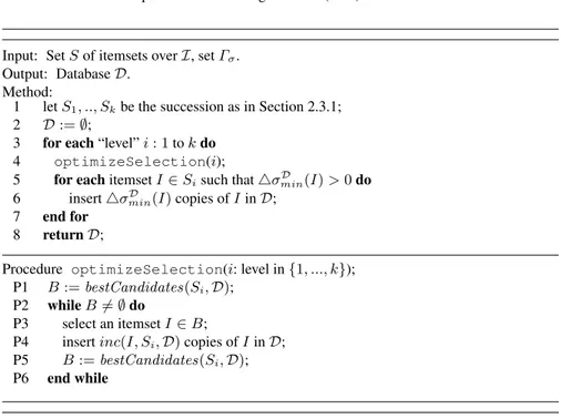
Input: Set S of itemsets overI, set Γσ.
Output: DatabaseD. Method:
1 let S1, .., Skbe the succession as in Section 2.3.1;
2 D := ∅;
3 for each“level” i : 1 to k do
4 optimizeSelection(i);
5 for eachitemset I∈ Sisuch that4σminD (I) > 0 do
6 insert4σDmin(I) copies of I inD;
7 end for 8 returnD;
Procedure optimizeSelection(i: level in{1, ..., k}); P1 B := bestCandidates(Si,D);
P2 while B6= ∅ do
P3 select an itemset I ∈ B;
P4 insert inc(I, Si,D) copies of I in D;
P5 B := bestCandidates(Si,D);
P6 end while
Fig. 2.1.Solution Algorithm for IFMS.
Firstly, we propose to process the itemsets of S that are candidates for being added to the output database D by means of a level-wise approach, where larger (w.r.t. set containment) itemsets are processed first. Formally, let S1, S2, .., Sk be a
succession of subsets of S such that: (i) Si∩Sj =∅ for each i 6= j; (ii)
Sk
i=1Si= S;
and, (iii) for each pair of subsets Siand Sjwith i < j, and for each itemset J ∈ Sj,
there is an itemset I ∈ Sis.t. I ⊃ J and there is no itemset I0 ∈ Si s.t. I0 ⊆ J.
Note that the succession S1, S2, .., Sk can efficiently be computed from S, and that
by processing itemsets according to their order of occurrence in the succession, we can enforce that each itemset is processed prior to its subsets.
Secondly, whenever processing the i-th element Si of the above succession and
for each itemset I ∈ Si, we propose to add inD the minimum possible number of
copies of I that suffices to satisfy σI
minand that do not lead to violate the maximum
support constraints on the subsets of I, which have in fact to be still processed. Formally, let ∆D(I) = minJ∈S|J⊂I(σmaxJ − σD(J )). Then, such number of copies
is given by the expression4σminD (I) = min(σI
min− σD(I), ∆D(I)). Note that one
may obtain4σDmin(I) ≤ 0, thereby implying that the algorithm fails in providing the minimum required support for I.
An algorithm implementing these ideas is shown in Figure 2.1. The input of the algorithm is a set of itemsets S and a set Γσ denoting the support constraints
associated with such itemsets. The output is a database with itemsets as transactions, which is meant as a heuristic solution to IFMS(I, S, Γσ).
2.3 A Level-Wise Solution Approach for IFMS 21
The algorithm starts by setting the databaseD to the empty set, and then applies the level-wise exploration of the itemsets in S in order to add elements intoD—for the moment let us get rid of step 4 that implements an optimization discussed in Section 2.3.2. In fact, given that each update onD preserves the maximum support constraint on all the subsets of the processed itemset and given that itemsets are processed according to their set inclusion, it is immediate to check that the resulting databaseD is such that for each item I ∈ S, σD(I)≤ σI
maxholds. However, we have
no theoretical guarantee on the fact that the minimum support constraint is satisfied over each itemset. In an extreme case, no copy of some itemset might be added toD even though a certain number of them are required.
As for the running time, note that the dominant operation in step 6 is repeated |S| times, i.e., once for each itemset in S. Moreover, computing ∆σD
min(I) requires
iterating over all the subsets of I, which are|S| at most. In total, O(|S|2× |I|) is a bound on the running time of the algorithm in Figure 2.1, where the|I| factor accounts for the cost of manipulating (e.g., comparing) itemsets composed by |I| items at most after an arbitrary ordering is fixed on them.
2.3.2 Optimization Issues
In the algorithmic scheme we have discussed, at each level i of the search, itemsets from Sionly are added intoD. In practice this might be too restrictive. Indeed, we
might think of enforcing the support of each itemset I ∈ Si by adding an itemset
J ⊃ I contained in some set Sjwith j < i, rather than by directly adding I. In fact,
note that such an itemset Sjis guaranteed to exists (except for i = 1), by construction
of the succession S1, ..., Sk.
This optimization founds on the idea that enforcing the support of I by includ-ing copies of one of its supersets has the side-effect of incrementinclud-ing the support of other itemsets included in J and, hence, belonging to same level subsequent to Sj.
This is very relevant in our approach, given that this effect goes in the direction of amplifying the chances of ending up with a database satisfying the minimum sup-port constraints over all itemsets, which is a critical issue as we discussed above. In practice, to implement this strategy, the algorithm in Figure 2.1 accounts for an optimization step that is performed before that itemsets at the current level Si are
analyzed. This optimization is next discussed in detail. Let4σmaxD (I) = min(σI
max− σD(I), ∆D(I)) be the maximum number of
copies of I that can be added toD while still satisfying σI
maxand while not violating
the maximum support constraints on the subsets of I. For any itemset I ∈ Sjand for
any element Siwith i > j, define then inc(I, Si,D) as the value:
min
4σmaxD (I), min I0∈ Si∧ I0⊂ I∧ σmin(I0) > σD(I0) (σImin0 − σD(I0)) .
Intuitively, this is the maximum increment allowed on the support of I computed by also considering as a bound the minimum support which suffices to satisfy the
constraints σIs
minon any of its subsets Isthat have still to be satisfied (i.e., for which
σIs
min> σD(Is) currently holds). In practice, we do want to increment the support of
I by affecting as less as possible the support of its subsets. Based on the increment values computed at the level associated with Si, we want to compute the set of all the
itemsets in some level below Sithat leads to reduce as much as possible the number
of itemsets to be added toD.
To this end, define first gainSet(I, S, J,D) as the itemsets whose minimum support is not yet satisfied and that are subsets of I and supersets of J , i.e., gainSet(I, S, J,D) = {I0 ∈ S | I0 ⊂ I ∧ I0 ⊃ J ∧ σI0
min < σD(I0)}. Define
then gain(I, Si, J,D) as the value:
inc(I, Si,D) ∗ (|gainSet(I, S, J, D)| − 1)
4σD max(I)
.
Intuitively, this is a normalized value that is meant to denote the advantage of adding inc(I, Si,D) copies of I to D w.r.t. an itemset J that have still to be
pro-cessed. By averaging this gain over all the itemsets that have to be processed, we define the value avgGain(I, Si,D) as:
P
J∈Sk
j=i+1Sj∧J⊃Igain(I, Si, J,D)
|Sk j=i+1Sj|
.
Finally, let bestCandidates(Si,D) be the set of all itemsets in
Si−1
j=1Sjon which the
maximum value (not equals to zero) of the average gain is achieved . These itemset are those that we consider the most promising for being added toD. These itemsets are computed in step P1 of the optimization procedure and updated in P5, after that inc(I, Si,D) copies of an
itemset I (arbitrarily picked from bestCandidates(Si,D)) have been actually added to D.
As for the running time, note that while without optimization we need to iterate only over the sets in|S| (as to compute ∆σDmin(I)), we now need to compute the set bestCandidates(Si,D)
which is feasible in O(|S2|). In total, the complexity is now O(|S3| × |I|).
2.3.3 An Example of computation
We conclude the description of the algorithm in Figure 2.1 by illustrating an example of com-putation over an IFMSproblem defined over the setI = {a, b, c, d} of items, and such that:
S ={I1, ..., I9} where I1={a, c, d}, I2={a, b, c}, I3={c, d}, I4={c, a}, I5={b, c},
I6 ={d}, I7 ={a}, I8 ={c}, and I9 ={b}; and where the functions σminand σmaxare
those defined in the following table:
I1 I2 I3I4 I5 I6 I7I8 I9
σmin 1 1 1 4 5 1 4 5 5
σmax 4 5 4 5 6 4 5 6 6
2.4 Solving the General Case of IFM 23 Note that itemsets in S can be arranged into the three levels S1, S2, and S3, as for they are graphically depicted in the topmost part of Figure 2.2. Thus, at the first iteration of the algorithm, all the elements in S1 are processed. No optimization can be performed on them since this is the first level of the hierarchy, and hence the algorithm performs steps 5 and 6 by updating the databaseD (initially empty) by adding one copy of I1and one copy of I2. In fact, note that4σminD (I1) =4σminD (I2) = 1.
In the second iteration, the algorithm processes the second level S2. This time, the optimization procedure can be applied to S1. Note that we have: gain(I1, S2, I6,D) =
gain(I1, S2, I7,D) = gain(I2, S2, I7,D) = 3∗(1−1)3 = 0, gain(I1, S2, I8,D) = gain(I2, S2, I8,D) = 3∗(2−1)
4 = 0.75, and finally gain(I2, S2, I9,D) = 3∗(1−1)
5 = 0.
Thus, avgGain(I1, S2, S3,D) coincides with the value:
gain(I1, S2, I6,D) + gain(I1, S2, I7,D) + gain(I1, S2, I8,D)
4 = 0,
whereas avgGain(I2, S2, S3,D) is the value:
gain(I2, S2, I7,D) + gain(I2, S2, I8,D) + gain(I2, S2, I9,D)
4 = 0.18.
It follows that, at the end of the second iteration, the algorithm updatesD by adding
inc(I2, S2,D) = 3 copies of I2 into D. The reader may now check that the subsequent iteration ends up by adding one copy of I5. After this update, the databaseD turns out to satisfy all the constraints (see the bottom part of Figure 2.2).
2.4 Solving the General Case of IFM
Now that a solution approach for IFMS has been described, we can move to discussing a
solution approach for the more general IFM problem. In fact, it it worthwhile observing that the algorithm in Figure 2.1 can already be seen as a heuristic approach to face IFM. Indeed, in addition to the specific heuristic used to deal with the support constraints, this algorithm heuristically solves IFM by restricting the set of all the possible transactions to those in S.
In practice, focusing on the set S might be too restrictive to solve IFM. Thus, we propose to enlarge the original set S by including various novel itemsets (built from those in S), whose exploitation is envisaged to be beneficial for improving the effectiveness of the algorithm in Figure 2.1.
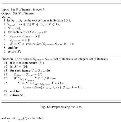
The approach, illustrated in Figure 2.3, constructs a novel set S0to be used as input for the algorithm in Figure 2.1 by merging k itemsets at most from S. The merging function is carried out recursively, by picking an itemset at time from a set of candidates itemsets (Scand).
In particular, it is worthwhile observing that itemsets are merged together if and only if their intersection is not empty (which motivates the initialization in step 2 and the check in F5). Indeed, this is in line with the approach discussed in Section 2.3.2, where the gain of two itemsets having no subset in common is equals to zero. In addition, note that the merging process is restricted to maximal itemsets only, i.e., to those which are included in the first level
S1.
We conclude the section by noticing that as for the support constraints, for each itemset
I∈ S(0, we set σmin0 (I) as the value:
σImin I∈ S
Input: Set S of itemset, integer k. Output: Set S0of itemset. Method:
1 let S1, .., Skbe the succession as in Section 2.3.1;
2 Scand={I ∈ S1|∃Y ∈ Si>1: Y ⊂ I};
3 S0={∅};
4 for each itemset I∈ Scanddo
5 Scand= Scand− {I};
6 Sf usion={I};
7 S0= S0∪ recursGen(Sf usion, Scand, k− 1);
8 end for 9 return S’;
Function recursGen(Sf usion, Scand: set of itemsets, k: integer): set of itemsets;
F1 if k = 0 then return{∅}; F2 let S∗={∅};
F3 for eachitemset I∈ Scanddo
F4 Scand= Scand− {I};
F5 if TY∈S
f usionY ∩ I 6= ∅ then
F6 S∗= S∗∪ {SY∈S
f usionY ∪ I} ∪
∪recursGen(Sf usion∪ {I}, Scand, k− 1);
F7 end for F8 return S∗;
Fig. 2.3.Preprocessing for IFM.
and we set σmax0 (I) as the value:
(
σmax(I) I∈ S
min(st, min(σ0max(Y )|Y ∈ S0∧ I ⊃ Y )), I /∈ S
where st is a user bound on the support of the new itemset.
Given these novel input specifications, the algorithm for IFMS0is then applied and used
as a heuristic approach to solve IFM on S. Eventually, note that for any fixed natural number
k, the above preprocessing step is not an overhead for the running time of the algorithm in
Figure 2.1.
2.5 Computational Result
The above solution approach for IFM has been implemented, and a thorough experiential activity has been conducted to assess its efficiency and effectiveness. Details on this activity are discussed in the remaining of the section.
2.5 Computational Result 25 2.5.1 Test instance
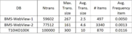
Experimentation is carried out over three distinct datasets [ZKM01], which have been often used as reference benchmarks for frequent itemsets discovery algorithms: The artificial dataset T10I4D100K, and the two real datasets BMS-WebView-1 and BMS-WebView-2. These latter databases contain clickstream data from two e-commerce web sites (each transaction repre-sents a web session and each item in a page viewed in that session). Summary information on these three datasets (in particular, the total number of transactions, the maximum transaction size, and the average transaction size, the number of distinct items, and the average frequency of an item) are illustrated in Table 3.4.
Fig. 2.4.Characteristics of used data set.
For each of the above databases, the idea of the experimentation is to firstly extract the set
S of the itemsets that are actually frequent (by standard itemsets discovery algorithms). For
each itemset I∈ S whose frequency is σ, we define σImin= σ−α∗σ and σmax= σ + α∗σ,
where α is a normalized real number (that will be varied in the experimentations). Then, the whole set S together with the support constraints constructed as above will be supplied as input to our algorithm for the IFM problem.
To evaluate the scalability of the algorithm we shall just refer to its running time. Instead, to evaluate its effectiveness in solving IFM, we shall take care of the following relative error index: er(%) = 1 |S|∗ X I∈S:σD(I)<σI min σminI − σD(I) σI min .
It is worthwhile observing that the above index accounts for how may itemsets from S occur in the output database with a support that is below the required constraint. In fact, recall from Section 2.3.1 that the maximum support constraint is always satisfied with our approach. Clearly enough, values of er(%) close to 0 are desirable.
All the results discussed below have been obtained by experimenting with an Intel dual core with 1.8GB memory, running windows XP Professional.
2.5.2 Results
A first series of experiment was aimed at assessing the scalability of our approach w.r.t. some key input parameters. In particular, we considered the real datasets BMS-WebView1 and BMS-WebView2 by varying the parameter α (from 0 to 0.3). Execution times are re-ported in Figures 2.5 and 2.6, for increasingly larger support and size of the set S. Note that execution times are not affected by the size of the interval over the support constraints.
In a second series of experiments, we assessed the effectiveness of the approach by com-puting the relative index error over the three detasets, by varying the support and the α param-eter. Results are reported in Figure 2.7. The figures evidence that the error rate is below 2%
(a) Increasingly larger support. (b) Increasingly larger set of input item-sets.
Fig. 2.5.Execution Times on BMS-WebView1 (for different α values).
(a) Increasingly larger support. (b) Increasingly larger set of input item-sets.
Fig. 2.6.Execution Times on BMS-WebView2 (for different α values).
for BMS-View-1 and T10I4D100K dataset, while is below 10% for BMS-View-2. It comes with no surprise that accuracy improves by increasing α. Moreover, it is relevant to notice that the error is always equals to 0 when α > 0.3, i.e., when a sufficiently large support constraint window is defined.
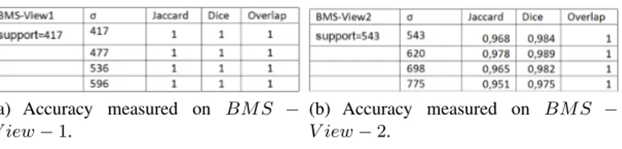
In a further set of experiments, we considered the experimentation perspective discussed in [WWWL05]. There, it is argued that the effectiveness of inverse frequent itemsets mining algorithms has to be assessed (1) by comparing the itemsets that can be actually rediscovered on the syntectic database with those occurring in the original one, and (2) by comparing the performances of a mining algorithm (e.g., Apriori) over the syntectic and the original dataset. In order to deal with (1) above, we used the Jaccard, Dice, and Overlap [WWWL05] indices to compare similarities between original frequent itemsets and those occurring in the syntectic output database. Results on the real input datasets are reported in Figure 2.8. The figure evidences that very high accuracy measures are obtained, and that support threshold values are greater or equal to the support threshold used for data generation.
Finally, as for (2), we report in Figure 2.9 the difference between execution times of Apriori when running on the original dataset and when running on the syntetic one (build on T10I4D100K by using the three supports values: 0.5, 0.6 and 0.7). Note that the lower is the support used in the generation of dataset, the smaller is the difference of performances.
2.5 Computational Result 27
(a) BMS-WebView1. (b) BMS-WebView2.
(c) T10I4D100K.
Fig. 2.7.Accuracy of the Approach.
(a) Accuracy measured on BM S −
V iew− 1.
(b) Accuracy measured on BM S −
V iew− 2.
Fig. 2.8.Accuracy Measured on Generated data.