Accounting and Economic Rates of Return: A Dynamic Econometric Investigation

EUI WORKING PAPERS

EUROPEAN UNIVERSIT Y INSTITU TE

Accounting and Economic Rates of Return:

A Dynamic Econometric Investigation

RODRIGO M. ZEIDAN

and

MARCELO RESENDE

D e p a r t m e n t o f E c o n o m i c s

EUROPEAN UNIVERSITY INSTITUTE

DEPARTMENT OF ECONOMICS

Accounting and Economic Rates of Return: a Dynamic Econometric Investigation

RODRIGO M.ZEIDAN

and

MARCELO RESENDE

This text may be downloaded freely only for personal academic purposes. Any reproductions, whether in hard copies or electronically, require the consent of the author. If cited or quoted,

reference should be made to the full name of the author(s), editor(s), the title, the working paper, or other series, the year and the publisher.

ISSN 1725-6704

© 2006 Rodrigo M. Zeidan and Marcelo Resende Printed in Italy

European University Institute Badia Fiesolana

I – 50016 San Domenico di Fiesole (FI) Italy

http://www.iue.it/

Accounting and Economic Rates of Return: a Dynamic Econometric

Investigation*

Rodrigo M. Zeidan

Escola de Gestão e Negócios , UNIGRANRIO

Rua da Lapa, 86, Centro, Rio de Janeiro-RJ, CEP: 20021-180 Email: rodrigo_zeidan@hotmail.com

Marcelo Resende

Visiting fellow, European University Institute and

associate professor

Instituto de Economia, Universidade Federal do Rio de Janeiro, Av. Pasteur 250, Urca, 22290-240, Rio de Janeiro-RJ

Email: mresende@ie.ufrj.br

Abstract

Many studies have questioned empirical utilization of accounting data as internal rates of return would be more consistent with the relevant economic concept. The paper investigates the dynamic relationships between different measures of accounting rates of return (ARRs) and different approximations for the internal rates of returns (IRRs). In contrast with the prevailing case-study investigations, one considers a panel for quoted Brazilian firms in the manufacturing industry along the 1988-3/2003-2 period. Granger causality tests are considered and even though the results are not completely clear cut, some discernible uni-directional patterns emerge. In particular, there seems to be informational content between economic and accounting rates of return, between ROA (Net Profits/Total Assets) and PM (Gross Profits/ Operational Income), and internal rates of return. This seems to indicate that there is some validity in using accounting rates of return in certain economic studies.

JEL Classification: M21, M41

* _{The second author acknowledges the hospitality of the European University Institute where part of}

1. Introduction

A whole body of economic literature deals with the differences between economic and accounting rates of return. Seminal papers date back to Harcourt (1965), Solomon (1966), Fisher and McGowan (1983) and Salamon (1985). The main conclusion is that there are fundamental differences between accounting and economics definition and measurement of rates of return. These differences arise from many sources: although advertising and research and development are considered investment from an economic viewpoint both are liabilities in the financial statement of firms; accounting depreciation is arbitrary, be it straight-line depreciation or reducing balance method and important intangible assets are not computed in financial statements (and are hard to compute economically).

Since then, many papers have dealt with empirical measures of economic and accounting rates of return [see e.g. Verma (1990), Bosch (1990), Chang et al (1994), Feenstra and Wang (2000), Taylor (1999), Salvary (2005)]. Some of those studies used this difference as a route towards the measurement of the real economic rate of return whereas others investigated the relationship between accounting and economic rates of return. The main results remain the same: there are irreconcilable differences between economic and accounting rates of return.

A disenchantment with the utilization of accounting rates of return for economic analysis became evident with the emergence of the so-called New Empirical Industrial Organization-NEIO that proposed indirect strategies of identifying market conduct without the need of marginal cost observability [see Bresnahan (1989) for an early account of that growing literature]. Nevertheless, the use of improved rates of return remains relevant in different contexts as for

example in the case of regulatory schemes that rely heavily on accounting data such as cost-plus and earnings sharing regimes.

The investigation of the relationship between accounting and economic rates of return and therefore the contribution of the present paper can be motivated at least in two levels:

a) In studies on the determinants of profitability a salient stylized fact refers to the robustness of the results with regard to different accounting rates of return [see Schmalensee (1989)]. However there is a gap in the literature in what concerns the empirical behavior of improved rates of return that attempt to proxy the internal rate of return;

b) Building on the previous point, one notes the absence of more systematic empirical studies that relate the aforementioned categories of rates of return as indeed the handful of related papers nearly have a case study character [see e.g. Taylor (1999)]

The present paper aims at partially filling the referred gap by considering a more comprehensive analysis of the relationship between accounting and economic rates of return by means of econometric methods. Even though the long-run behavior of the different measures display strong co-movements, it is important to properly portray the short-run dynamic associations between the different measures of rates of return. Specifically, we consider a Granger causality analysis for a panel of quoted Brazilian industrial firms.

The paper is organized as follows. The second section introduces the conceptual aspects related to the calculation of the conditional IRRs necessary for the test, and the set of accounting rates of return to be considered. The third section presents the data construction procedures and the results for the rates of

return in terms of the dynamic relationships among those indicators. The fourth section brings some final comments.

2. Accounting and Economic Rates of Return: Conceptual Aspects

2.1 The Conditional IRRs

To try to establish the long term relationship between accounting rates of return (ARRs) and the internal rate of return (IRR) the main problem is having the IRR to compare it to the ARRs. Let Yn be the revenue and In the investment, then

the IRR of a project is defined as the rate r that solves: 0 ) 1 ( ... 1 1 1 0 0 = + − + + + − + − n n_n r I Y r I Y I Y (1)

The IRR is then the rate that equals the present value of the investment with the cash flow that it generates, thus turning the present value of the investment zero. It could be considered the economic depreciation (Schmalensee, 1989), since depreciation distributes the value of investment over time. Thus the IRR can be considered a good proxy for the real unobserved economic return, since a project would only be viable if its IRR would be higher than a control parameter – usually the cost of capital.

Although conceptually easy to follow, empirical measurement of the IRR is not simple to do. Three are the main reasons:

• Equation (1) is a n-polynomial with n possible solutions. Thus for non-conventional cash flows there would be multiple IRRs with no possible way to determine which one would be the proxy for the economic rate of return (Ross et alli, 1998);

• Investment projects with the same IRR may not be interchangeable, since investment decision contemplates other aspects such as uncertainty or the need for initial investment. Thus a project that needs less investment should be preferable to a project with the same IRR but higher initial investment. • Since financial reports have many idiosyncrasies, and it is difficult to retrieve

which information is essential to build Yn and In .

Salamon (1982,1985) and Taylor (1995) tried to estimate the IRR by using Ijiri’s (1978) concept of Cash Recovery Rate (1978) to measure an indirect economic rate of return, and so we will follow those works and arrive at a IRR indirectly through the cash recovery rate (CRR).

The concept of the CRR was first developed by Ijiri (1978) as an alternative to the conventional ARRs. The rationale was that since the ARR did not measure cash flows in the economic sense, having the CRR would allow analysis of a firm’s cash flow and thus would be complementary to the regular information presented in financial reports. The CRR then shows the pattern of recoveries from a firm and is defined as: TASS DEPR TASS LTASS INTEXP INCBD CRR= + −∆ +∆ + (2)

with DEPR being depreciation; INCBD the sum of income from operations; INTEXP interest expenses; ∆LTASS book-value of long-term assets disposed; TASS is the average total asset of the period considered. The numerator represents the firm’s flow of recoveries, while the denominator is a stock variable. Thus the CRR reveal information on the recovery of the firm, with measures of flow and stock being

considered. Taylor (1999) includes research and development and advertisement in the CRR to allow for better recovery estimates to the pharmaceutical industry that was being studied. Since R&D and advertisement expenditures are not always published in financial reports we considered manufacturing industrial sectors to calculate its respective CRRs and conditional IRRs.Examples of those sectors are steel, pulp, mining, fertilizers mechanical and electrical machines among others. The choice was as ample as possible, contemplating any quoted company that did not operate in sectors with significant R&D and advertisement expenditures.

Salamon (1982,1985) showed that under some circumstances the CRR could be a proxy for the IRR of a firm, and thus estimates the relationship between the CRR and IRR as:

      − + − + +       − + − + − + = ) ) 1 (( ) 1 ( ) 1 ( ) 1 ( ) 1 ( ] 1 ) 1 /[( n n n n _{n n} b r b r r b g b g g g CRR (3)

with g being a constant that represents the growth of a firm’s investment over time;

n the life-time of the representative project of the firm; b a cash flow linear profile

that shows if recoveries for the firm’s investments increase, decrease, or are constant over time; r is the IRR of the typical project of the firm.

Equation (3) presents some strong assumptions: each firm is a collection of projects with similar IRRs, life-times, and cash-flow patterns; and the rate of investment growth of the firm is linear. These hypotheses are needed either to make calculation possible due to financial reports restrictions or to deal with inherent problems with IRRs, such as multiple results – for instance, a linear cash-flow pattern is needed to force a single IRR for each firm.

Furthermore, the cash-flow pattern, b, is crucial to estimation of equation (3). If Y0,Y1,...,Yn is the cash-flow of the representative project of the firm, with Y0 < 0 and

Y1,...,Yn > 0, then b is such that Yi = bi-1Y1, for i = 1,...,n. Thus the cash-flow profile

b relates past and future cash flows. If b < 1 (>1), the cash flow diminishes (grows)

exponentially. If b = 1, the recovery process is constant. Salamon (1985) argued that b could be estimated using information on past recoveries for the firms, but used ad hoc profiles of 0,8; 1,0; 1.1; and a random value between (0,8;1,1), arriving then at four conditional IRRs1.

Taylor (1999) derives a cash-flow profile for pharmaceutical firms based on the concept of summation point. The rationale is that investment processes are not perfectly perceived by financial reports due to the fact that it takes place over more than a year. The idea behind the summation point is thus at which point the firm starts to recover the investment is necessary to construct its cash-flow profile. For the pharmaceutical industry the number is 5 years – thus recoveries start at the start of the 5th year of the investment process of the industry. The main problem with this approach is that it requires too much industry-specific information.

Since later in the paper we will consider a panel data approach for testing Granger causality test, Taylor’s (1999) approach becomes untenable. In fact, it requires a detailed knowledge of each specific sector considered. That case study approach uses subjective information that is not readily available for a large number of sectors as in a panel data study. Although there will be ad hoc cash-flow profiles as

1 _{One important observation is that if the growth of investment is greater than the recoveries}

calculation of the IRR is impossible (Salamon, 1987). This is straightforward, since any calculation in finance requires negative and positive values for present and future values – and if recovery is never greater, then all Yn – In will be negative and thus will be impossible to derive a r that solves

in Salamon (1985) we will construct a firm-specific cash-flow profile to have another conditional IRR to use in the causality test and to avoid the fact that if there is no recovery a conditional IRR can not be estimated. The cash-flow profiles will then use past firm information. The rationale is that if investments are growing more than recoveries then recoveries will need to grow more rapidly in the future for the firm to recover its investment, and thus will have an increasing (>1) cash-flow profile. On the other hand, if recoveries are much bigger than investments firms should have a declining cash-flow profile. Using only income from operations are recoveries and investment, the firm-specific cash-flow profile is defined as:

∑

∑

Expression (4) then defines b as a relationship between the realized growth of investments and recoveries. The result leads to four conditional IRRs dependent on the values of b (0.8; 1; 1.1; and the firm-specific, which from now on are dubbed IRR1, IRR2, IRR3 and IRR4). Estimate the conditional IRRs is then solving (3). Taking:       − + − + − + = ) 1 ( ) 1 ( ] 1 ) 1 /[( * b g b g g g CRR W n n n ₍₄₎

Substituting (4) into (3) implies that solving (3) in terms of r is:

n n W b r W b r ) 1 ( + − − − = (5)

2,2- Accounting rates of returns

There is no previous information about a preferential ARR to try to establish the long term relationship between ARRs and IRR. Therefore, nine ARRs were constructed based on the most used ARRs. As table 1 indicates, the ARRs can be categorized as measures of return on assets, return on equity, profit margin, and asset turnover. Also, since there are three measures of profit in Brazilian financial reports: gross profit, earning before interest, taxes, depreciation and amortization (EBITDA) and net profit. For the first two categories we calculated three ARRs, while for return on equity we left out EBITDA.

INSERT TABLE 1 AROUND HERE

Thus nine ARRs were used for comparison with the conditional IRRs: • ROA – Gross Profits /Total Assets (1),

• ROA - Ebitda/Total Assets – (2), • ROA – Net Profits/Total Assets (3),

• PM – Gross Profits/ Operational Income (4), • PM – Net Profits/Operational Income (5), • PM – Ebitda/Operational Income (6), • ROE – Net Profits/Equities (7), • ROE – Gross Profits/Equities (8),

Next, the paper considers dynamic relationships among the different rates of return stressing aspects of stationarity and causality.

3. Empirical Analysis 3.1- Data construction

The data were obtained from Economatica, with quarterly financial reports for quoted companies from 1988 to 2003. To get a balanced panel with complete data the period considered was from the third quarter of 1988 through the second quarter of 2003, comprising 60 time periods. The total number of firms was 155, with only industrial firms from mature, low R&D2 sectors being chosen, to try to avoid the biggest discrepancies between ARRs and IRRs3_{. The results for the}

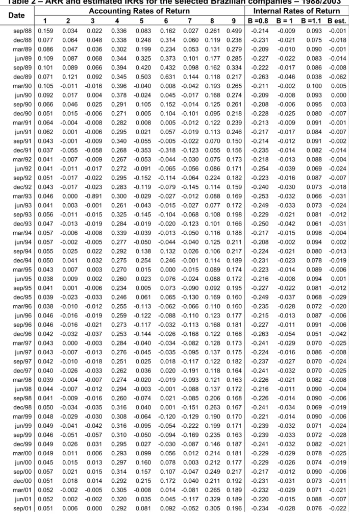
average IRRs and ARRs are presented in table 2.

INSERT TABLE 2 AROUND HERE

2 _{R&D is not a significant source of concern for discrepancies between ARRs and IRRs for Brazilian}

firms, since the average expenditure of R&D in Brazil is 0,4% of GDP, compared to the 2% of GDP in most industrialized countries (Rocha and Fernandes, 2001, IEDI, 2004).

3 _{Although this makes for a biased comparison between ARRs and IRRs, it could be justified for}

being the first exploratory test between its long run relationship. Also, it allows for a better control of the test, since if for the selected industrial firms no relationship were to be found this could be extended to the more intensive in R&D and advertising expenses’ firms.

From table 2 some information can be derived from the ARRs and IRRs for the Brazilian group of selected firms4. The ROA for the Ebitda was roughly zero for all the period considered. This is interesting and corroborates the view of the two lost decades of the 80’s and 90’s in Brazil.

In their seminal study, Fisher and McGowan (1983) used ROA measures, while Long and Ravenscraft argued that Fisher and McGowan (1983) erred for not using profit margins, which is more commonly used. To prevent any such problems, no a priori ARR is considered the best one to compare it to the IRRs estimated, and therefore the Granger causality tests, later considered, will consider all ARRs and IRRs.

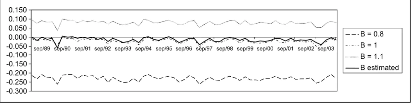
In the figure 1 the conditional IRRs clearly show co-movement, which was expected. Also, for b = 0.8 for every period the average IRR is negative, which was also expected since a small value of b means that the cash-flow of the average should decrease which would in turn mean that most recovery would have already taken place and hence a negative IRR. An important observation is that the estimated conditional IRR is very consistent with an approximate value of b = 1.

INSERT FIGURE 1 AROUND HERE

4 _{Just as a comparison, for the same period the average ROA for the American manufacturing}

sector was 4.7%, profit margin 4.5%, and return on equities 11.9% (Bureau of the Census, "Quarterly Financial Report for Manufacturing, Mining, and Trade Corporations"- 2004).

The ARRs are much more erratic, as expected and shown on graph 2. Some values are necessarily positive, as AT and Gross Profit Margin, others have a negative mean, as Net ROE, and surprisingly Net PM is stable throughout the period.

INSERT FIGURE 2 AROUND HERE.

Also, it is interesting to note that in many periods the average Net Profit Margin (PM) presents a higher value than the Ebitda PM. This can be explained by long periods of very high interest rates, which implicates disinvestment processes, with profits from operations being transformed in interest payments. Usually financial considerations would not be so important in a analysis for a large number of firms, but Brazilian economy experienced some periods of real interest rates of over 20%, as from 1996-98.

3.2- Causality analysis

The previous graphical depiction of the different rates of return made clear that long-run co-movements are present among those variables. Nevertheless, we consider stationarity tests so as to rule out the possibility of spurious regressions in the later econometric analysis. In fact, we consider unit root tests for heterogeneous panels as proposed by Im, Pesaran and Shin-IPS (2003). The corresponding results are reported in appendix 1 and largely favors the prevalence

of I(0) variables and therefore one does not need to further pursue co-integration analysis.

Hence, we can focus on exploring short-term relationships between pairs of rates of return. However, unlike the usual time series setting for testing causality, we face a data set with a panel structure that should be fully explored.

The Granger causality notion is by now well established in [see Granger (1969)]. Let Yt and Xt denote stationary stochastic processes observed through

time t and let _σ2(.) _{indicate the variance of the conditional linear least squares} forecast of a given stochastic process. X is said to ’Granger cause’ Y (X ⇒ Y but not Y ⇒ X) if and only if σ2_(Y

t|Y,X) < σ2(Yt|Y) where Y and X denote

information on past realizations of the two stochastic processes. Bidirectional causality would, of course, arise when causality prevails in both directions. In summary, Granger causality arises when past realizations of X improve the prediction of Y and in that sense usual empirical implementations rely on joint statistical tests of lagged coefficients of regressors. In the context of panel data, however, only a handful of applications can be found. Examples include Holtz-Eakin et al (1988) who investigated inter-temporal linkages between local government expenditures and revenues in the U.S. and Banerjee (2003) explores causal patterns between incentive regulation and service-quality in U.S. telecommunications. This latter work takes advantage of a GMM efficient estimator for dynamic panels. In fact, the asymptotic bias of utilizing traditional panel data estimators in dynamic models have legitimated alternative estimators with an instrumental variable structure. Among those, the GMM estimator proposed by Arellano and Bond-AB (1991) is an efficient estimator especially useful for short

panels. Before proceeding with the Granger causality tests, it is important to consider auxiliary specification tests:

a) In order to make consistency of the estimator tenable, one has to be assured that second order serial correlation is not present. For that purpose the test proposed by AB is useful.

b) The lagged variables in levels that are used instruments for the model estimated in first-difference must be deemed as valid. In that sense, a test of over-identifying restrictions along the lines of Sargan (1958) is relevant. Under the null hypothesis of validity of the instruments the test statistic is distributed as χ2_{(r), where r denotes the difference between the instrument}

rank Z and the number of estimated coefficients.

The results for both specification tests are presented in the appendix 2 and were satisfactory indicating that we can safely proceed with the Granger causality tests. Table 3 summarizes the corresponding results.

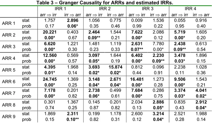
INSERT TABLE 3 AROUND HERE

We perform the analysis for possible combinations of rate of returns. It was expected that if there were causality between ARRs and IRRs, it should be between the same kind of ARRs, like gross or net measures of account profitabilities. The results are mixed in that respect, with a strong unidirectional Granger causality from ARR to IRR between two ROAs measures (2 and 3), all PM measures (4,5,6), and ROE – Net Profits/Equities (7). Also there are unclear unidirectional Granger causality between some conditional IRRs and some ARRs, but there is no discernible pattern, since it would be expected that if there were

causality it would be between all IRR for the same ARR. The only salient result is that IRRs 3 and 4 Granger cause ARR 8 (ROE – Gross Profits/Equities), and IRRs 1 and 3 against ARR 9 (Income from operations /Total Assets). Also, it is worth noticing that there are some bi-directional results, between IRR2 and ARRs 5 and 6.

The main result is then that there seems to be informational content between economic and accounting rates of return, in this case, between ROA and PM and internal rates of return. This seems to indicate that there is some validity in using accounting rates of return in economic studies, especially when long time series are considered.

4. Final Considerations

Many papers deal with differences between accounting and economic rates of return (e.g. Fisher and McGowan (1982) and Salamon (1985) among others). The goal of the paper was to delve into the subject to verify whether within a dynamic structure of analysis, the differences between accounting and economic rates of return are so important to render accounting rates of return irrelevant for economic modeling. The paper contrasts with the previous literature by exploring the panel structure of the data set comprising different sectors and therefore departing from the previously adopted case-study framework. In particular, we try to verify if accounting rates of return could be salvaged on the grounds of being leading indicators of internal rates of return or vice-versa.

The main difficulty was estimating the IRRs, that in any case require strong hypothesis for being constructed. In order to undertake the investigation, we used a dynamic panel data approach with a GMM estimator for testing Granger

causality. The motivation was to detect eventual informational content between series of internal rates of return and accounting rates of return so as to discern differences between the series and infer possible implications towards economic modeling.

Even though the results did not present completely clear cut patterns, it were interesting because showed at least a unidirectional causality between ROA and PM rates of return and the internal rates of return estimated.

The tendency in studies of market power assessment is to bypass the use of accounting data by considering indirect methods of conduct measurement based in oligopoly models. Nevertheless, the evidence obtained in present paper is in part encouraging for the use of accounting rates of return in economic analysis as for example in regulated settings that traditionally rely to a great extent in that type of data.

References

Arellano, M., Bond, S. (1991), Some tests of specification for panel data: Monte Carlo evidence and an application to employment equations, Review of Economic

Studies, 58, 277-297

Baltagi, B.H. (2005), Econometric Analysis of Panel Data, 3rd _{ed., New York: John}

Wiley & Sons

Banerjee, A. (2003), Does incentive regulation ‘cause’ degradation of retail telephone service quality?, Information Economics and Policy, 15, 243-269

Bresnahan, T.F. (1989), Empirical studies of industries with market power, in R.Schmalensee and R.D. Willig (eds.), Handbook of Industrial Organization, Amsterdam: North-Holland, 1011-1057

Bureau of the Census, (2004) Quarterly Financial Report for Manufacturing, Mining, and Trade Corporations.

Chang, C.S.A., Kite, D. and Radtke, R. (1994), The applicability and usage of NPV and IRR capital budgeting techniques. Managerial Finance, 20, 7, 10-16.

Feenstra, D. and Wang, H., (2000). Economic and accounting rates of return,

Research Report 00E42, University of Groningen, Research Institute SOM.

Fisher, F.M., and McGowan, J.J., (1983). On the misuse of accounting rates of return to infer monopoly profits, American Economic Review, 73, 82-97.

Fisher, F., (1984). On the misuse of accounting rates of return: a reply. American

Economic Review, 74.

Fisher, F.M., (1987). On the misuse of the profit-sales ratio to infer monopoly power, Rand Journal of Economics, 18, 384-96.

Granger, C.W. (1969), Investigating causal relations by econometric models and cross-spectral methods, Econometrica, 37, 424-438

Holtz-Eakin, D., Newey, W., Rosen, H.S. (1988), Estimating vector autoregressions with panel data, Econometrica, 1371-1395

Im, K.S., Pesaran, M. and Shin, Y., (2003), Testing for unit roots in heterogeneous panels, Journal of Econometrics, 115, 53-74

Ijiri, Y., (1978). Cash-Flow accounting and its structure, Journal of Accounting,

Auditing, and Finance, 1, 331-48.

Ijiri, Y., (1980). Recovery rate and cash flow accounting, Financial Executive, 48, 54-60.

Lee, T. A. and Stark, A., (1987). Ijiri’s cash flow accounting and capital budgeting,

Accounting and Business Research, 17, 125–132.

Long, W.F. and Ravenscraft, D.J., (1984). The usefulness of accounting profit data: A comment on Fisher and McGowan, American Economic Review 74, 494-500. Martin, S., (1984). The misuse of accounting rates of return: Comment, American

Economic Review 74, 501-506.

Martin, S., (1988). The measurement of profitability and the diagnosis of market power, The International Journal of Industrial Organization 6, 301-321.

Moody, C., (2004). Notes on unit root tests with panel data, (http://cemood.people.wm.edu/panelur.pdf)

Ross, S.A., Westerfield, R.W. and Jordan, B.D., (1998). Fundamentals of corporate finance 4th Edition, Boston: McGraw Hills.

Salamon, G. L., (1982). Cash recovery rate and measures of firms profit,

Salamon, G. L., (1985). Accounting rates of return, American Economic Review,

75, 495–504.

Salamon, G. L., (1988). On the validity of accounting rate of return in cross sectional analysis: theory, evidence, and implications, Journal of Accounting and

Public Policy, 7, 267–292.

Salamon, G. L., (1989). Accounting rates of return: reply, American Economic

Review, 79, 290–93.

Salvary, C. W. S., (2005). Financial accounting information and the relevance/irrelevance issue, Finance 0502016, Economics Working Paper Archive

at WUSTL

Sargan, D. (1958). The estimation of economic relationships using instrumental variables, Econometrica, 26, 393-415

Schmalensee, R., (1989). Inter-industry studies of structure and performance, in R. Schmalensee and R.D. Willig (eds.), Handbook of Industrial Organization. Amsterdam: North Holland, 951-1009

Taylor, C., (1999). The cash recovery method of calculating profitability: an application to pharmaceutical firms, Review of Industrial Organization, 14, 135– 146.

Verma, K., (1990). Effects of accounting techniques on the study of market power,

Figure 1 – Conditional IRRs for the group of Brazilian firms selected.

Figure 2 – Accounting Rates of Return for Selected Brazilian Firms.

-0.600 -0.400 -0.200 0.000 0.200 0.400 0.600 0.800 set/8 8 set/8 9 set/9 0 set/9 1 set/9 2 set/9 3 set/9 4 set/9 5 set/9 6 set/9 7 set/9 8 set/9 9 set/0 0 set/0 1 set/0 2 set/0 3

lucro bruto/ ativo total LAIR/Ativo Total Lucro Liquido/Ativo Total Lucro Operacional/Ativo Total Lucro Bruto/Receita Líquida de Vendas Lucro Líquido/Receita Líquida de Vendas Lucro Operacional/Receita Líquida de Vendas Lucro Líquido/Patrimônio Liquido Lucro Bruto/Patrimônio Liquido -0.300 -0.250 -0.200 -0.150 -0.100 -0.050 0.000 0.050 0.100 0.150

sep/89 sep/90 sep/91sep/92 sep/93 sep/94 sep/95 sep/96 sep/97 sep/98 sep/99 sep/00 sep/01 sep/02sep/03

B = 0.8 B = 1 B = 1.1 B estimated

Table 1 – Different Accounting Rates of Return (ARRs).

Return on Assets (ROA)

Profit Margin

(Gross and Net)

Return on Equity (ROE)

Total Asset Turnover Profit

TASS INCBD Profit Equity Profit INCBD TASS How much profit

per $100 of investment.

How much profit per $100 of sales.

How much profit per $100 of proprietary

investment.

How much sales per $100 of firm’s

Table 2 – ARR and estimated IRRs for the selected Brazilian companies – 1988/2003

Accounting Rates of Return Internal Rates of Return

Date 1 2 3 4 5 6 7 8 9 B =0.8 B = 1 B =1.1 B est. sep/88 0.159 0.034 0.022 0.336 0.083 0.162 0.027 0.261 0.499 -0.214 -0.009 0.093 -0.001 dec/88 0.077 0.064 0.048 0.338 0.248 0.314 0.060 0.119 0.238 -0.231 -0.021 0.075 -0.018 mar/89 0.086 0.047 0.036 0.302 0.199 0.234 0.053 0.131 0.279 -0.209 -0.010 0.090 -0.001 jun/89 0.109 0.087 0.068 0.344 0.325 0.373 0.101 0.177 0.285 -0.227 -0.022 0.083 -0.014 sep/89 0.101 0.089 0.066 0.394 0.420 0.432 0.098 0.162 0.334 -0.222 -0.017 0.086 -0.008 dec/89 0.071 0.121 0.092 0.345 0.503 0.631 0.144 0.118 0.217 -0.263 -0.046 0.038 -0.062 mar/90 0.105 -0.011 -0.016 0.396 -0.040 0.008 -0.042 0.193 0.265 -0.211 -0.002 0.100 0.005 jun/90 0.092 0.017 0.004 0.378 -0.024 0.045 -0.017 0.168 0.274 -0.209 -0.008 0.093 0.000 sep/90 0.066 0.046 0.025 0.291 0.105 0.152 -0.014 0.125 0.261 -0.208 -0.006 0.095 0.003 dec/90 0.051 0.015 -0.006 0.271 0.005 0.104 -0.101 0.095 0.218 -0.228 -0.025 0.080 -0.007 mar/91 0.064 -0.004 -0.008 0.282 0.008 0.005 -0.012 0.122 0.239 -0.213 -0.009 0.091 -0.001 jun/91 0.062 0.001 -0.006 0.295 0.021 0.057 -0.019 0.113 0.246 -0.217 -0.017 0.084 -0.007 sep/91 0.043 -0.001 -0.009 0.340 -0.055 -0.005 -0.022 0.070 0.150 -0.214 -0.012 0.091 -0.002 dec/91 0.037 -0.055 -0.058 0.268 -0.353 -0.318 -0.123 0.055 0.156 -0.235 -0.014 0.082 -0.014 mar/92 0.041 -0.007 -0.009 0.267 -0.053 -0.044 -0.030 0.075 0.173 -0.218 -0.013 0.088 -0.004 jun/92 0.041 -0.011 -0.017 0.272 -0.091 -0.065 -0.056 0.086 0.171 -0.254 -0.039 0.069 -0.024 sep/92 0.051 -0.017 -0.022 0.295 -0.152 -0.114 -0.064 0.224 0.182 -0.223 -0.016 0.087 -0.007 dec/92 0.043 -0.017 -0.023 0.283 -0.119 -0.079 -0.145 0.114 0.159 -0.240 -0.030 0.073 -0.018 mar/93 0.046 0.000 -0.891 0.300 -0.029 -0.027 -0.012 0.088 0.169 -0.253 -0.032 0.066 -0.031 jun/93 0.041 0.003 -0.001 0.261 -0.043 -0.015 -0.027 0.077 0.172 -0.249 -0.033 0.073 -0.024 sep/93 0.056 -0.011 -0.015 0.325 -0.145 -0.104 -0.068 0.108 0.198 -0.229 -0.021 0.081 -0.012 dec/93 0.047 -0.013 -0.019 0.284 -0.019 -0.020 -0.123 0.101 0.166 -0.250 -0.042 0.061 -0.031 mar/94 0.057 -0.006 -0.008 0.339 -0.039 -0.013 -0.050 0.116 0.188 -0.217 -0.015 0.098 -0.004 jun/94 0.057 -0.002 -0.005 0.277 -0.050 -0.044 -0.040 0.125 0.211 -0.208 -0.002 0.094 0.002 sep/94 0.055 0.025 0.022 0.292 0.138 0.132 0.026 0.106 0.217 -0.224 -0.021 0.080 -0.013 dec/94 0.050 0.041 0.032 0.275 0.254 0.246 -0.001 0.114 0.189 -0.231 -0.023 0.078 -0.019 mar/95 0.043 0.007 0.003 0.270 0.015 0.000 -0.015 0.089 0.174 -0.223 -0.014 0.089 -0.006 jun/95 0.038 0.009 0.002 0.260 0.023 0.076 -0.024 0.088 0.172 -0.216 -0.008 0.094 0.001 sep/95 0.041 0.001 -0.006 0.234 0.005 0.073 -0.090 0.092 0.195 -0.227 -0.022 0.081 -0.012 dec/95 0.039 -0.023 -0.033 0.246 0.061 0.065 -0.130 0.169 0.160 -0.249 -0.037 0.068 -0.029 mar/96 0.038 -0.010 -0.012 0.255 -0.113 -0.062 -0.066 0.110 0.160 -0.235 -0.028 0.072 -0.020 jun/96 0.046 -0.016 -0.019 0.259 -0.122 -0.088 -0.110 0.123 0.177 -0.215 -0.013 0.087 -0.006 sep/96 0.046 -0.016 -0.021 0.273 -0.117 -0.032 -0.113 0.168 0.181 -0.227 -0.011 0.091 -0.006 dec/96 0.042 -0.032 -0.037 0.253 -0.144 -0.026 -0.168 0.122 0.168 -0.263 -0.054 0.051 -0.042 mar/97 0.043 0.000 -0.003 0.284 -0.040 -0.034 -0.082 0.128 0.173 -0.241 -0.029 0.070 -0.025 jun/97 0.043 -0.007 -0.013 0.276 -0.045 -0.035 -0.095 0.137 0.175 -0.224 -0.016 0.086 -0.008 sep/97 0.042 -0.010 -0.018 0.251 0.025 0.018 -0.117 0.122 0.182 -0.237 -0.027 0.070 -0.024 dec/97 0.040 -0.026 -0.033 0.262 0.036 0.020 -0.191 0.118 0.164 -0.241 -0.032 0.070 -0.025 mar/98 0.039 -0.004 -0.007 0.274 -0.020 -0.019 -0.093 0.121 0.163 -0.226 -0.021 0.082 -0.008 jun/98 0.044 -0.007 -0.012 0.294 -0.003 -0.001 -0.088 0.137 0.172 -0.216 -0.011 0.090 -0.004 sep/98 0.041 -0.009 -0.016 0.260 -0.074 0.021 -0.085 0.206 0.168 -0.226 -0.014 0.090 -0.006 dec/98 0.050 -0.034 -0.035 0.316 0.040 0.001 -0.151 0.263 0.167 -0.241 -0.034 0.069 -0.019 mar/99 0.048 -0.029 -0.030 0.308 -0.064 -0.120 -0.129 0.190 0.170 -0.221 -0.014 0.090 -0.006 jun/99 0.049 -0.041 -0.042 0.316 -0.095 -0.054 -0.222 0.199 0.171 -0.239 -0.032 0.071 -0.024 sep/99 0.046 -0.051 -0.057 0.310 -0.050 -0.094 -0.169 0.235 0.163 -0.239 -0.033 0.072 -0.028 dec/99 0.049 0.026 0.031 0.295 0.027 -0.030 -0.087 0.146 0.187 -0.241 -0.032 0.082 -0.021 mar/00 0.049 0.011 0.006 0.293 0.099 0.056 0.012 0.214 0.181 -0.229 -0.029 0.078 -0.025 jun/00 0.045 0.015 0.013 0.297 0.160 0.078 0.003 0.212 0.177 -0.229 -0.026 0.074 -0.019 sep/00 0.057 0.021 0.015 0.314 0.157 0.107 -0.047 0.249 0.217 -0.217 -0.012 0.090 -0.006 dec/00 0.051 0.018 0.014 0.292 0.215 0.172 0.040 0.211 0.192 -0.231 -0.031 0.073 -0.011 mar/01 0.052 -0.002 -0.005 0.305 -0.008 0.014 -0.081 0.265 0.189 -0.232 -0.029 0.071 -0.021 jun/01 0.052 0.002 -0.002 0.320 0.035 0.045 -0.117 0.329 0.189 -0.220 -0.015 0.088 -0.007 sep/01 0.051 0.006 0.000 0.292 0.081 0.092 -0.052 0.305 0.196 -0.234 -0.028 0.076 -0.022

dec/01 0.049 0.028 0.025 0.278 0.269 0.253 0.016 0.300 0.188 -0.233 -0.023 0.076 -0.017 mar/02 0.048 0.000 -0.004 0.286 0.021 0.043 -0.110 0.207 0.191 -0.232 -0.026 0.077 -0.018 jun/02 0.054 -0.027 -0.031 0.326 -0.022 -0.021 -0.268 0.325 0.191 -0.225 -0.021 0.084 -0.012 sep/02 0.047 -0.062 -0.068 0.320 -0.117 -0.072 -0.331 0.281 0.169 -0.254 -0.050 0.051 -0.031 dec/02 0.058 -0.037 -0.043 0.308 -0.029 0.062 -0.352 0.407 0.216 -0.248 -0.045 0.054 -0.041 mar/03 0.049 0.014 0.006 0.277 0.016 0.077 0.020 0.256 0.209 -0.222 -0.024 0.076 -0.015 jun/03 0.052 -0.009 -0.017 0.282 0.095 0.154 -0.082 0.383 0.215 -0.208 -0.010 0.089 -0.004 Average 0.055 0.002 -0.019 0.296 0.024 0.046 -0.067 0.169 0.200 -0.229 -0.023 0.079 -0.015

Table 3 – Granger Causality for ARRs and estimated IRRs.

IRR 1 IRR 2 IRR 3 IRR 4

arr ⇒ irr irr ⇒ arr arr ⇒ irr irr ⇒ arr arr ⇒ irr irr ⇒ arr arr ⇒ irr irr ⇒ arr stat 1.757 2.896 1.056 0.775 0.009 1.536 0.055 0.916 ARR 1 prob 0.17 0.06* 0.35 0.46 0.99 0.22 0.95 0.40 stat 20.221 0.403 2.464 1.544 7.622 2.086 5.719 1.605 ARR 2 _{prob 0.00* 0.67 0.09** 0.21 0.00* 0.12 0.00* 0.20} stat 6.620 1.221 1.481 1.119 2.631 7.780 2.438 0.613 ARR 3 _{prob 0.00* 0.30 0.23 0.33 0.07** 0.00* 0.09** 0.54} stat 12.560 0.569 3.097 1.644 6.402 2.230 3.478 1.896 ARR 4 prob 0.00* 0.57 0.05* 0.19 0.00* 0.09** 0.03* 0.15 stat 4.395 1.968 3.693 15.874 0.812 0.096 2.238 1.028 ARR 5 _{prob 0.01* 0.14 0.02* 0.02* 0.44 0.91 0.11 0.36} stat 24.745 1.369 3.148 2.671 16.481 1.273 9.506 1.543 ARR 6 _prob 0.00* 0.25 0.04* 0.04* 0.00* 0.28 0.00* 0.21 stat 7.178 0.201 2.738 0.499 7.684 0.286 3.374 4.041 ARR 7 prob 0.00* 0.82 0.06* 0.61 0.00* 0.75 0.03* 0.02* stat 0.301 1.367 0.145 0.201 2.034 2.886 0.835 2.912 ARR 8 _{prob 0.74 0.25 0.87 0.82 0.13 0.05* 0.43 0.04*} stat 1.869 2.311 0.199 1.178 2.600 3.214 2.521 1.988 ARR 9 _{prob 0.15 0.10** 0.82 0.31 0.12 0.04* 0.28 0.14}

Appendix 1

Unit Root test results for the CRR, ARRs and IRRs.

IPS ARR1 -20.7387 ARR2 -77.7027 ARR3 -56.8323 ARR4 -14.1748 ARR5 -27.0421 ARR6 -22.9106 ARR7 -16.8325 ARR8 -17.1219 ARR9 -8.16017 ARR10 -21.254 CRR -71.0371 IRR1 -42.5761 IRR2 -47.7185 IRR3 -46.664 IRR4 -48.2777

The critical value for the IPS (2003) test, with confidence interval of 5%, N = 93 and

Appendix 2

Sargan, and LM First and Second Order Serial Correlation test results.

IRR 1 IRR 2 IRR 3 IRR 4

arr ⇒ irr irr ⇒ arr arr ⇒ irr irr ⇒ arr arr ⇒ irr irr ⇒ arr arr ⇒ irr irr ⇒ arr Sargan 90.32/93 91.58/94 86.45/93 90.66/94 89.29/96 92.51/95 90.87/93 91.08/93 p value 0.02 0.02 0.00 0.01 0.00 0.03 0.01 0.03 AR1/p 1.34/0.00 2.20/0.01 7.99/0.09 4.09/0.05 7.17/0.08 2.85/0.04 0.95/0.00 2.41/0.02 ARR 1 AR2/p 49.8/0.85 10.1/0.12 89.0/0.95 22.1/0.37 9.1/0.10 28.9/0.44 15.8/0.25 20.5/0.35 Sargan 90.88/93 92.22/96 90.49/93 92.34/94 90.52/94 90.80/93 91.19/94 89.98/93 p value 0.02 0.03 0.02 0.05 0.02 0.02 0.04 0.01 AR1/p 5.24/0.06 2.11/0.03 2.26/0.03 4.33/0.05 7.75/0.09 2.31/0.03 1.02/0.01 0.59/0.00 ARR 2 AR2/p 14.8/0.52 29.0/0.73 46.5/0.84 38.5/0.69 36.5/0.61 49.2/0.84 109/0.99 24.3/0.43 Sargan 92.12/96 91.48/94 91.23/95 91.03/94 90.39/93 91.88/95 90.01/94 90.45/93 p value 0.04 0.03 0.03 0.03 0.03 0.03 0.01 0.03 AR1/p 1.23/0.01 0.72/0.00 0.69/0.00 1.01/0.01 1.82/0.02 1.32/0.01 0.79/0.00 1.01/0.01 ARR 3 AR2/p 75.6/0.93 79.8/0.95 20.0/0.24 27.6/0.40 35.4/0.65 26.5/0.40 66.9/0.95 39.2/0.66 Sargan 89.75/92 89.21/93 88.21/92 90.33/93 90.81/95 90.08/96 89.02/93 92.25/95 p value 0.02 0.01 0.01 0.03 0.02 0.01 0.03 0.04 AR1/p 0.88/0.00 0.94/0.01 1.88/0.02 1.11/0.01 1.09/0.01 1.21/0.01 6.10/0.07 3.91/0.05 ARR 4 AR2/p 29.0/0.32 31.3/0.36 54.8/0.81 31.6/0.30 49.8/0.77 63.3/0.92 57.6/0.81 62.9/0.74 Sargan 90.88/93 86.22/95 90.48/93 90.01/93 87.56/92 90.22/93 91.23/93 84.88/93 p value 0.03 0.00 0.03 0.03 0.01 0.03 0.05 0.00 AR1/p 1.88/0.02 2.89/0.04 1.00/0.01 2.73/0.04 0.66/0.00 5.21/0.06 7.81/0.09 1.53/0.02 ARR 5 AR2/p 27.6/0.41 59.2/0.78 56.6/0.73 88.5/0.97 22.2/0.34 32.8/0.56 18.7/0.15 44.3/0.53 Sargan 90.54/93 88.67/92 90.19/93 91.57/94 88.90/93 92.09/96 90.87/93 86.58/92 p value 0.03 0.01 0.03 0.03 0.01 0.03 0.03 0.00 AR1/p 1.22/0.01 0.91/0.00 1.04/0.01 3.94/0.05 3.77/0.05 5.69/0.07 1.94/0.02 0.55/0.00 ARR 6 AR2/p 91.2/0.96 51.1/0.62 84.6/0.95 24.2/0.29 81.0/0.97 108/0.99 96.9/0.98 41.8/0.58 Sargan 91.02/94 90.44/93 89.90/93 90.39/93 90.28/93 91.10/94 90.80/93 90.62/93 p value 0.03 0.03 0.02 0.03 0.03 0.03 0.03 0.03 AR1/p 1.21/0.01 0.88/0.00 0.49/0.00 1.39/0.02 1.27/0.01 1.09/0.01 0.62/0.00 1.01/0.01 ARR 7 AR2/p 35.2/0.48 36.6/0.55 34.7/0.54 79.9/0.97 51.0/0.52 38.0/0.42 15.1/0.12 27.7/0.33 Sargan 90.55/93 90.82/93 89.89/94 90.08/94 90.00/93 90.28/93 90.22/95 90.18/93 p value 0.03 0.03 0.02 0.03 0.03 0.03 0.01 0.03 AR1/p 0.66/0.00 1.78/0.02 1.12/0.01 1.21/0.01 0.98/0.00 3.91/0.05 0.80/0.00 1.10/0.01 ARR 8 AR2/p 23.6/0.28 41.0/0.55 52.1/0.69 94.0/0.99 90.2/0.98 18.0/0.18 81.5/0.96 20.0/0.26 Sargan 89.08/94 91.92/96 88.28/92 92.45/96 89.06/94 89.90/93 90.29/93 91.22/94 p value 0.02 0.01 0.01 0.03 0.00 0.03 0.03 0.03 AR1/p 0.77/0.00 1.07/0.01 1.17/0.01 2.88/0.04 1.02/0.01 2.47/0.04 2.43/0.03 2.19/0.03 ARR 9 AR2/p 50.2/0.69 29.6/0.31 63.3/0.89 58.4/0.84 81.0/0.94 42.7/0.58 72.8/0.90 39.6/0.51

Note: the Sargan results reported are the test statistic and instrument rank (that gives the degrees of freedom) in the first row and the p-value in the second. The results for the AR1 and AR2 are the test statistics and the corresponding p-values.