SCUOLA DOTTORALE IN INGEGNERIA Dottorato di ricerca in Scienze dell'Ingegneria Civile
______________________________________________________
SCUOLA DOTTORALE / DOTTORATO DI RICERCA IN
XXVII CICLO
_______________________
CICLO DEL CORSO DI DOTTORATO
Uniaxial Material Model for Reinforcing Bar Including
Buckling in RC Structures
__________________________________________________
Titolo della tesi
Zhihao Zhou
__________________________ __________________
Nome e Cognome del dottorando
firmaProf. Camillo Nuti
_________________________ __________________
Docente Guida/Tutor: Prof.
firmaProf. Aldo Fiori
________________________ __________________
Collana delle tesi di Dottorato di Ricerca In Scienze dell’Ingegneria Civile
Università degli Studi Roma Tre Tesi n° 55
Abstract
The constitutive model of steel reinforcing bar incorporating inelastic buckling is crucial to accurate seismic performance evaluation of the existing reinforced concrete structures. According to experimental observations, in presence of inelastic buckling the absolute maximum stress of the rebar in compression could reduce to half of the value in absence of buckling.
In this thesis, based on fiber element model, the effect of the yield strength on the critical slenderness of the rebar is studied. Then the formulas, incorporating the effect of yield stress, are given to calculate the computational slenderness critical slenderness. Next the anisotropy of some stainless steel rebar is studied according to a series of monotonic and cyclic tests on bare stainless steel rebars. Two parameters are proposed to consider the effects of anisotropy of rebar.
Considering the above studies, the modified Monti-Nuti Model is proposed to improve the applicability. In order to eliminate overestimation of stress when the model is subjected to generalized loading, the criteria to update the parameters in the model for each half branch at the reversal are discussed and new strategies to update the model parameters in different unloading or reloading cases are proposed. The Framework adopting Genetic Algorithm is designed to identify the parameters in the modified Monti-Nuti model. By minimizing the stress difference between the numerical curve and experimental curve at each strain step of the cyclic loading histories, the optimized parameters could be identified. Then the empirical formulae are proposed to calculate the values of the parameters in a simpler, more efficient and still robust way. The modified Monti-Nuti model is implemented into OpenSees as a new material model named as “steel05”. Then validation of this material model with the experimental curves of carbon steel rebars and stainless steel rebars confirms the effectiveness and significance of this new model. Furthermore, the application of the new material in the structural analysis of circular reinforced concrete piers is made and the numerical curves are compared with the experimental curves to verify the effectiveness of the new material.
Finally, the effects of corrosion of the rebar, which is inevitable in aged reinforced concrete structures, are studied based on a series of experiments on the bare corroded reinforcing bars. It is found that the mean yield stresses of the corroded rebar could be different in tension and
in compression. The computational length of the rebar increases resulting from the deterioration of the confinement from the transverse loop. The corrosion extended model is proposed to consider the aforementioned characteristics resulting from corrosion.
Contents
LIST OF FIGURES ... IX LIST OF TABLES ... XVI LIST OF SYMBOLS ...XVII
1. INTRODUCTION ... 1
1.1 BACKGROUNDS ... 1
1.1.1 Importance of Inelastic Buckling ... 2
1.1.2 Rebar Applied in the Concrete Structures ... 5
1.2LITERATUREREVIEW ... 5
1.2.1 Cyclic Steel Model for Rebar ... 6
1.2.2 Steel Model Incorporating Inelastic Buckling ... 14
1.3SIGNIFICANCEANDAIMSOFCURRENTRESEARCH ... 18
1.3.1 Significance ... 18
1.3.2 Aims of Current Research... 19
1.4ORGANIZATION OF THIS THESIS ... 19
2. ORIGINAL MONTI-NUTI MODEL ... 20
2.1MONOTONICSKELETONCURVE ... 20
2.2HARDENINGRULESFORCYCLICBEHAVIORSOFSTEELREBAR ... 23
2.2.1 In Absence of Buckling ... 23
2.2.2 In Presence of Buckling ... 27
2.3CURVETRANSITIONPARAMETERR ... 31
2.3.1 In Absence of Buckling ... 32 2.3.2 In Presence of Buckling ... 32 2.4HARDENINGRATIO ... 33 2.4.1 In Absence of Buckling ... 34 2.4.2 In Presence of Buckling ... 34 2.5ELASTICMODULUSE ... 35 2.5.1 In Absence of Buckling ... 35 2.5.2 In Presence of Buckling ... 35
3. IMPROVEMENT OF THE ORIGINAL MODEL ... 37
3.1EFFECTOFYIELDSTRESSONCRITICALSLENDERNESS ... 44
3.1.1 Fiber Model Adopted in Microanalysis of Bare Bar ... 45
3.1.2 Verification of the Fiber Model ... 55
3.1.3 Combined Factor Affecting Critical Slenderness ... 58
3.3MODIFIEDMONTI-NUTIMODEL ... 62
3.3.1 Effect of the Yield Strength ... 63
3.3.2 Effect of the Anisotropy ... 63
3.4ADDITIONALCRITERIAFORUPDATETHEMODELPARAMETERS ... 65
3.4.1 Discussion of the Proposed Solutions to Address the Above Issues ... 65
3.4.2 Proposed Criteria to Update the Model Parameters under Generalized Loading... 70
4. PARAMETER IDENTIFICATION BY GENETIC ALGORITHM ... 83
4.1 INTRODUCTION OF PARAMETER IDENTIFICATION BY GENETIC ALGORITHM ... 83
4.1.1 Parameter Identification ... 83
4.1.2 Genetic Algorithm ... 85
4.2DESIGNOFPARAMETERIDENTIFICATIONOFMODIFIEDMONTI-NUTI MODEL ... 85
4.2.1 Parameters to Be Calibrated ... 86
4.2.2 Flowchart ... 86
4.2.3 Objective Function ... 88
4.2.4 Bounds of the Parameters ... 88
4.3EFFECTIVENESSOFTHEOPTIMIZEDPARAMETERS ... 89
4.3.1 Stress-Strain Curve ... 89
4.3.2 Step-Stress Comparison ... 92
4.3.3 Robustness ... 94
4.4 PROPOSED FORMULAS FOR THE PARAMETERS IN THE MODIFIED MONTI-NUTIMODEL ... 96
5. IMPLEMENTATION AND VALIDATION OF THE MODIFIED MONTI-NUTI MODEL ... 97
5.1IMPLEMENTTHEMATERIALMODELINOPENSEES... 97
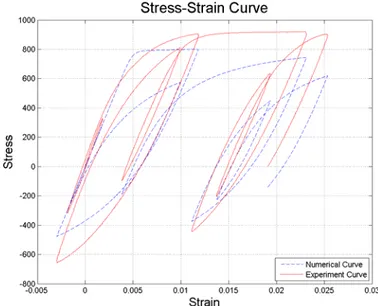
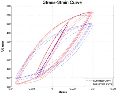
5.2VALIDATION OF THE MODIFIED MONTI-NUTI MODEL ... 98
5.2.1 Experiments of Carbon Steel Rebar ... 101
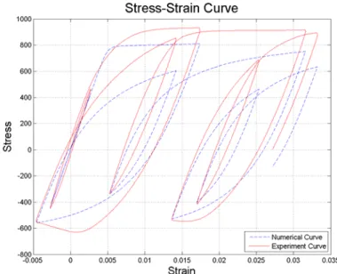
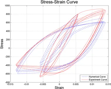
5.2.2 Experiments of Stain Steel Rebar ... 109
6. APPLICATION IN REINFORCED CONCRETE COLUMN ... 114
6.1APPLICATIONOFFIBERMODELINCANTILEVERCOLUMNANALYSIS ... 114
6.2PSEUDO-DYNAMICTESTOFREINFORCEDCONCRETEBRIDGEPIER 115 6.2.1 Regular Reinforced Concrete Bridge Pier ... 115
6.3COMPARISON BETWEEN THE NUMERICAL ANALYSIS AND EXPERIMENTAL RESULTS ... 118
6.3.1 Main Parameters in the Fiber Model ... 118
6.3.2 Experimental Test of the Bridge Piers ... 119
6.3.3 Comparisons Between Numerical Curves and Experimental Curves ... 122
7.1MECHANISMOFCORROSION OFREBAR INREINFORCEDCONCRETE
... 125
7.2EFFECTOFCORROSION ... 131
7.2.1 EFFECT OF CORROSION ON YIELD STRESS ... 132
7.2.2 Effect of Corrosion on Critical Slenderness ... 137
7.2.3 Effect of Corrosion on Computational Length of Rebar ... 139
7.3CORROSIONEXTENDEDMODELFORREBAR ... 140
7.3.1 Notional Yield Stresses in Tension and Compression ... 141
7.3.2 Slenderness Ratio of Corroded Rebar ... 142
8. CONCLUSIONS AND FURTHER WORKS ... 147
8.1CONCLUSIONS ... 147
8.2FURTHERWORKS ... 149
ACKNOWLEDGEMENTS ... 151
List of figures
Figure 1.1 Fiber Element Method ... 1
Figure 1.2 Bearing capacity of column ... 2
Figure 1.3 Theoretical model for the reinforced bar in the concrete columns (Gomes & Appleton, 1997) ... 3
Figure 1.4 The effect of the inelastic buckling on the stress-strain curve .. 4
Figure 1.5 Cyclic model proposed by Aktan et al. (1973) ... 7
Figure 1.6 Cyclic model for rebar proposed by Ma et al. (1976) based on Ramberg-Osgood model ... 8
Figure 1.7 Cyclic stress-strain curve with envelope proposed by Thompson and Park (1978) based on Ramberg-Osgood model ... 9
Figure 1.8 Cyclic stress-strain curve with envelope proposed by ... 10
Figure 1.9 Cyclic model proposed by Aktan and Ersoy (1980) ... 10
Figure 1.10 Menegotto-Pinto Model ... 12
Figure 1.11 Modified Menegotto-Pinto model ... 13
Figure 1.12 Combination of Gomes and Appleton Model ... 14
Figure 1.13 Monotonic Skeleton curve proposed by Dhakal and Maekawa(2002b) ... 16
Figure 1.14 Schematic Diagram of rebar in Concrete Column ... 17
Figure 1.15 Trilinear Model proposed by Zong (2010) ... 18
Figure 2.1 Monotonic tests of carbon steel rebar (Giorgio Monti & Nuti, 1992) ... 20
Figure 2.2 Monotonic skeleton curve of Monti-Nuti model ... 22
Figure 2.3 Effect of strain hardening in absence of buckling ... 24
Figure 2.4 Effect of strain hardening in presence of buckling ... 28
Figure 2.5 Stress shift in compressive curve ... 31
Figure 2.7 The effect of b on the curve transition ... 33
Figure 2.8 Degradation of elastic modulus ... 35
Figure 3.1 Comparison between experimental curve and numerical curve generated by original Monti-Nuti model (S5, L/D=5) ... 38
Figure 3.2 Comparison between experimental curve and numerical curve generated by original Monti-Nuti model (S8, L/D=8) ... 38
Figure 3.3 Comparison between experimental curve and numerical curve generated by original Monti-Nuti model (S11, L/D=11) ... 39
Figure 3.4 Monotonic tests on stainless steel rebar (AISI304 or 1.4301) 40
Figure 3.5 Comparison between experimental curve and numerical curve generated by original Monti-Nuti model (Stainless steel rebar, XA1, L/D=5) ... 41
Figure 3.6 Comparison between experimental curve and numerical curve generated by original Monti-Nuti model (Stainless steel rebar, XA2, L/D=5) ... 41
Figure 3.7 Comparison between experimental curve and numerical curve generated by original Monti-Nuti model (Stainless steel rebar, XA3, L/D=5) ... 42
Figure 3.8 Comparison between experimental curve and numerical curve generated by original Monti-Nuti model (Stainless steel rebar, XC1, L/D=11) ... 43
Figure 3.9 Comparison between experimental curve and numerical curve generated by original Monti-Nuti model (Stainless steel rebar, XC2, L/D=11) ... 43
Figure 3.10 Comparison between experimental curve and numerical curve generated by original Monti-Nuti model (Stainless steel rebar, XC3, L/D=11) ... 44
Figure 3.11 Fiber technique in simulating the bare rebar ... 45
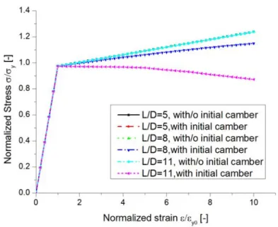
Figure 3.12 Comparisons between monotonic compressive curves of rebar generated by fiber model with or without initial imperfection ... 47
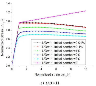
Figure 3.13 Comparisons between the monotonic curves of rebar with different slenderness (L/D) generated by fiber model with different initial imperfections ... 49
Figure 3.14 Comparisions between monotonic curves of rebar with different slendernesses generated by fiber model using different numbers of elements ... 50
Figure 3.15 Comparisions between monotonic curves of rebar with different slendernesses generated by fiber model using different numbers of Integration Points for each element ... 52
Figure 3.16 Comparisions between monotonic curves of rebar with different slendernesses generated by fiber model adopting different numbers of subdivisions along the circle and the radius for cross section meshing ... 54
Figure 3.17 Verification of the fiber model with monotonic compressive experimental curves with different slendernesses ... 55
Figure 3.18 Loading strain histories of cyclic test A1 and C1 ... 56
Figure 3.19 Verification of the fiber model with the experimental cyclic stress-strain curves of rebar with differernt slendernesses ... 57
Figure 3.20 Effect of yield stress on the stress-strain curves of rebar with different slenderness and yield stress generated by fiber model .. 59
Figure 3.21 Monotonic stress-strain curves of rebar with different combined parameters generated by fiber model ... 59
Figure 3.22 Testing machine and the specimen: a) Test machine MTS 810; b) specimen in tension; c) specimen in compression ... 61
Figure 3.23 Update curvature parameter R in the case of partial unloading and reloading ... 66
Figure 3.24 Solution to eliminate the overestimation under partial unloading and reloading (Attolico et al., 2000) ... 67
Figure 3.25 Solution to eliminate the overestimation under partial unloading and reloading ... 69
Figure 3.26 Fiber technique and applied in Finite Element Method (Dhakal & Maekawa, 2002c) ... 70
Figure 3.27 Different types of positions of reversal ... 72
Figure 3.28 Status of branch n+1: Plastic, UL/RL, AB/PB; ... 73
Figure 3.29 Status of branch n+1: Elastic, UL, AB/PB; ... 76
Figure 3.30 Status of branch n+1: Elastic, RL, AB; ... 77
Figure 3.31 Status of branch n+1: Elastic, RL, PB; ... 78
Figure 3.32 Status of branch n+1: Small, UL, AB/PB; ... 80
Figure 3.33 Status of branch n+1: Small, RL, AB; ... 81
Figure 3.34 Status of branch n+1: Small, RL, PB; ... 82
Figure 4.1 General flowchart of parameter identification ... 84
Figure 4.2 Parameter identification of modified Monti-Nuti model ... 87
Figure 4.3 Comparison between experimental curve and numerical curve generated by modified Monti-Nuti Model (carbon steel rebar, A1, L/D=5) ... 90
Figure 4.4 Comparison between experimental curve and numerical curve generated by modified Monti-Nuti Model (carbon steel rebar, C1, L/D=11) ... 90
Figure 4.5 Comparison between experimental curve and numerical curve generated by modified Monti-Nuti Model (stainless steel rebar, XA1, L/D=5) ... 91
Figure 4.6 Comparison between experimental curve and numerical curve generated by modified Monti-Nuti Model (stainless steel rebar, XC1, L/D=11) ... 91
Figure 4.7 Step-Stress comparison between experimental curves and numerical curve with optimized parameters (carbon steel rebar, L/D=5, A1) ... 92
Figure 4.8 Step-Stress comparison between experimental curves and numerical curve with optimized parameters (carbon steel rebar, L/D=11, C1) ... 93
Figure 4.9 Step-Stress comparison between experimental curves and numerical curve with optimized parameters (stainless steel rebar, L/D=5, XA1) ... 93
Figure 4.10 Step-Stress comparison between experimental curves and numerical curve with optimized parameters (stainless steel rebar,
L/D=11, XC1) ... 94
Figure 4.11Derivations of optimized parameters ... 96
Figure 5.1 Inheritance Diagram of steel model “Steel05” ... 98
Figure 5.2 Column setup in OpenSees for material test ... 99
Figure 5.3 Scripts used to test “Steel05” in OpenSees ... 100
Figure 5.4 Loading strain histories of carbon steel reinforcement ... 101
Figure 5.5 Comparison of numerical curves and experimental curves (L/D=5) ... 104
Figure 5.6 Comparison of numerical curves and experimental curves (L/D=11) ... 106
Figure 5.7 Loading strain histories of carbon steel reinforcement ... 107
Figure 5.8 Comparison of numerical curves and experimental curves (S5, L/D=5) ... 107
Figure 5.9 Comparison of numerical curves and experimental curves (S8, L/D=8) ... 108
Figure 5.10 Comparison of numerical curves and experimental curves (S11, L/D=11) ... 108
Figure 5.11 Loading strain histories of stainless steel reinforcement .... 110
Figure 5.12 Comparison of numerical curves and experimental curves (L/D=5) ... 111
Figure 5.13 Comparison of numerical curves and experimental curves (L/D=11) ... 113
Figure 6.1 Fiber element technique used in reinforced concrete pier analysis under cyclic loading ... 114
Figure 6.2 Regular bridge ... 116
Figure 6.3 Pier Specimen corresponding to the middle pier in the regular bridge ... 116
Figure 6.5 Lateral loading displacement histories at the top of the pier 120
Figure 6.6 Experimental lateral force and displacement curve of pier 1 121
Figure 6.7 Experimental lateral force and displacement curve of pier 5 121
Figure 6.8 Comparison of force-displacement curve (horizontal force at the bottom and lateral displacement at the top of pier) between the
fiber model and the experimental curves ... 122
Figure 6.9 Comparison of force-displacement curve (horizontal force at the bottom and lateral displacement at the top of pier) between the fiber model and the experimental curve ... 123
Figure 7.1 Corrosion of rebar in the highway bridge: a) corrosion of the pier b)corrosion of the rebar and spalling of the cover concrete of the wall c) overview of the highway bridge (Tullmin, 2010) ... 125
Figure 7.2 corrosion of rebar in concrete (Tullmin, 2010)... 127
Figure 7.3 Stage 1 of corrosion (Tullmin, 2010)... 128
Figure 7.4 Stage 2 of corrosion (Tullmin, 2010)... 128
Figure 7.5 Stage 3 of corrosion (Tullmin, 2010)... 129
Figure 7.6 Stage 4 of corrosion (Tullmin, 2010)... 129
Figure 7.7 Electrochemical reaction of rebar in concrete ... 130
Figure 7.8 Notional yield stress deterioration in tension and compression (L/D=5) ... 134
Figure 7.9 Notional yield stress deterioration in tension and compression (5<L/D<=10) ... 134
Figure 7.10 Notional yield stress deterioration in tension and compression (L/D>10) ... 135
Figure 7.11 Relationship between mean yield stress and mass loss rate L/D=5, data from Kashni et al. (2013a) ... 136
Figure 7.12 Relationship between mean yield stress and mass loss rate L/D=10, data from Kashni et al. (2013a) ... 136
Figure 7.13 Relationship between mean yield stress and mass loss rate L/D=15, data from Kashni et al. (2013a) ... 137
Figure 7.14 Ratio between the critical slenderness of corroded rebar and critical slenderness of original rebar '
cr cr
... 138
Figure 7.15 Buckling of compressed bar between two consecutive stirrups ... 139
Figure 7.16 Buckling exceeds two consecutive stirrups ... 140
Figure 7.17 Stress-strain relationship of corroded rebar with different slenderness ... 143
Figure 7.18 Relationship between ' (ratio computational slenderness of corroded rebar and original rebar) and mass loss rate ... 144
List of tables
Table 3.1Properties of test rebar (Dhakal & Maekawa, 2002b) ... 37
Table 3.2 Content of chemical composition in stainless steel AISI304 ... 40
Table 3.3 Selection of Parameters for Fiber Model ... 54
Table 3.4 Geometric and Mechanical properties of bare rebar ... 55
Table 3.5 Parameters values of “Steel02” adopted in the fiber model ... 56
Table 3.6 Combined parameter for different rebars ... 58
Table 3.7 Possible conditions of the previous branch ... 71
Table 3.8 Stragety for model update at reversal ... 72
Table 4.1 Lists of parameters to be calibrated ... 86
Table 4.2 Lower bound and Upper bound of the parameters ... 89
Table 4.3 Parameter Identification for stainless steel rebar (L/D=5) ... 95
Table 4.4 Parameter Identification for stainless steel rebar (L/D=11) ... 95
Table 5.1 Properties of tested carbon steel rebar ... 101
Table 5.2 Properties of test rebar (Dhakal and Maekawa 2002) ... 106
Table 5.3 Properties of tested stainless steel rebar ... 109
Table 6.1 Geometries and configuration of the piers ... 117
Table 6.2 Mechanical properties of the materials tested in the laboratory ... 118
Table 6.3 Parameters of “Concrete07” in the fiber model ... 119
Table 6.4 Parameters of “Steel05” in the fiber model ... 119
Table 7.1 Parameters to calculate the notional yield stress deterioration ... 133
List of symbols
Nell’elenco che segue sono riportati i principali simboli che compaiono nei capitoli della tesi.
Computational slenderness
L Computational length
D Diameter of the cross section of rebar
E Elastic modulus
0
E Initial tangent modulus
Stress
Strain
i Raidus of gyration
r
,
L D
cr Critical slenderness between inelastic buckling and elasticbuckling
r
Critical stress between inelastic buckling and elastic buckling
p
Critical slenderness between plastic and inelastic buckling
p
Critical stress between plastic and inelastic buckling
i
Initial stress at the beginning of the half cycle
i
Initial strain at the beginning of the half cycle
0
0
, y Yield strain
*
Normalized stress in Menegotto-Pinto model
*
Normalized strain in Menegotto-Pinto model
b Hardening ratio used in Menegotto-Pinto model, equaling
the ratio between the tangent modulus of the asymptote after yielding point and the initial tangent modulus at the original point or reversal point
n r
Stress corresponding to the reversal point
n r
Strain corresponding to the reversal point
1
n y
Stress corresponding to the yield point of the n+1 half
cycle
1
n y
Stain corresponding to the yield point of the n+1 half cycle
n
Plastic excursion at the n th semi cycle normalized by the strain y corresponding to the initial yield stress f y
R Curve transition parameter defined in Menegotto-Pinto
model
0
R Initial curve transition value defined in Menegotto-Pinto
model
1
A ,A 2 Parameters to calculate R , defined in Menegotto-Pinto
model
st
Stress shift due to isotropic strain hardening
max
Absolute maximum value at the reversal of previous half cycles
3
a , a 4 Experimentally determined parameters to calculate stress
shift proposed by Filippou et al.
s
Normalized superposition length, representing the distance between the tensile curve and the monotonic compressive curve after the yield point, defined in Monti-Nuti model
*
s
Real superposition length
0
b Initial hardening ratio in tension, defined in Monti-Nuti
model
0
b Initial hardening ratio in compression, defined in
Monti-Nuti model
b Hardening ratio in tension b Hardening ratio in compression
i
p
Plastic strain hardening at the i th half cycle
max
Maximum plastic strain hardening of previous half cycles
n p
Plastic work of n th half cycle
n K
Stress variation due to kinematic strain hardening at n th half cycle
n I
Stress variation due to isotropic strain hardening at n th half cycle
n p
Additional plastic excursion
n IM
Stress variation due to isotropic strain hardening and memory rule, defined in Monti-Nuti model, in absence of buckling
made by the kinematic rule and the isotropic rule
n KM ,b
Stress variation due to kinematic strain hardening and memory rule in presence of buckling, defined in Monti-Nuti model
sh
Stress shift defined in Monti-Nuti model
0
b
R Initial value of curve transition parameter in presence of
buckling, defined in Monti-Nuti model
1
b
A ,A 2b Parameter to calculate R in presence of buckling, defined
in Monti-Nuti model
1
b
R Lower bound of R in presence of buckling, defined in
Monti-Nuti model
The limitation value of the asymptote for softening branch
The sum of additional plastic excursion of previous half cycles
L D fy Computational slenderness
450
y
L D F Computational critical slenderness Parameter anisotropy coefficient
Critical slenderness coefficient
Y
f Yield stress of Feb44, equaling 450 MPa yt
f Yield strength of rebar in tension yc
f Yield stress of the rebar in compression
1t
modified Monti-Nuti model
1
c
A , A2c Parameters to calculate R in compressive half branch,
defined in modified Monti-Nuti model
t
r , r c Parameters to calculate the initial value of R , defined in 0
modified Monti-Nuti model
n
The set of controlling parameters in the model for n th half branch
f Fitness function
k
f Value of the fitness function for each experimental curve
Y
The difference between the numerical curve and the experimental curve
Y Sum of the square of the experimental stresses at each strain steps
,
E i
y , yN i, Stress on the experimental curve and numerical curve
corresponding to the same strain
k
w Weight coefficient for each experimental curve
'
D Mean cross section of the corroded rebar
c
Mass loss rate due to corrosion
Mass loss rate due to corrosion, in percentage 0
m Original mass of the rebar m Mass of corroded rebar
'
yt
f Yield stress in tension corresponding to the corroded rebar
a Regression factor to calculate '
yt
f , representing the effect
of non-uniform pitting corrosion
'
yc
f Yield stress in compression corresponding to the corroded
rebar based on the mean cross section area
c
Regression factor to calculate '
yc
f , representing the effect
of non-uniform pitting corrosion
t c
d Notional yield stress deterioration in tension due to
corrosion
c c
d Notional yield stress deterioration in compression due to
corrosion
'
cr
Critical slenderness of corroded rebar corresponding to mean yield stress '
yc
f '
Slenderness of the corroded rebar corresponding to mean yield stress '
yc
f
'
L Computational length of the corroded rebar t
c
Corrosion deterioration factor incorporating the effect of non-uniform pitting corrosion in tension
c c
Corrosion deterioration factor incorporating the effect of non-uniform pitting corrosion in compression
g Gap distance generated at the contact point between the
stirrup and the longitudinal rebar due to corrosion
s
D Diameter of the uncorroded stirrup
'
s
D Diameter of the uncorroded stirrup
due to corrosion
''
Slenderness of the corroded rebar based on the cross section of the original uncorroded rebar
''
cr
Critical slenderness of the corroded rebar based on the cross section of the original uncorroded rebar
c deterioration coefficient to calculate fyc which is the
notional yield stress in compression corresponding to the corroded rebar
1. INTRODUCTION
The material model for rebar including inelastic buckling is crucial for precise seismic performance evaluation of existing reinforced concrete structures. Through literature review, the state of art of steel material model for rebar in reinforced concrete structures is introduced. Subsequently the significance of this research is demonstrated, and finally the organization of this thesis is briefly explained.
1.1 BACKGROUNDS
There are many existing concrete structures designed before the effect of earthquake was fully studied. The stirrup spacing in existing structures exceeds the maximum limit specified in the current seismic code, thus the confinement of the transverse stirrups towards the longitudinal reinforcement is not sufficient, which will result in the lateral deformation of the longitudinal rebar named as buckling after the collapse of the concrete cover under severe seismic loading.
Figure 1.1 Fiber Element Method
In order to evaluate the seismic performance of these reinforced concrete structures, the finite element method adopting fiber element model is
widely applied to reduce the computational cost. As shown in Figure 1.1, the concrete column or beam is divided into segments along the axial length, and the cross section of the segment is further divided into fibers which represent concrete and rebar (Mullapudi, 2010). Supposing that the plane section remains plan, the strain in each fiber is calculated from the centroidal section strain and curvature. Subsequently the stresses and modulus of fibers are calculated from the fiber strain. The constitutive relation of the section is derived by integration of the response of the fibers. Furthermore, the response of the element is derived by integration of the response of the sections along the length of the element.
In the fiber element model, proper material models for concrete and steel reinforcing bar take very important roles. Subjected to seismic action, the structures suffer repeated loading and unloading and the elements of the structures could undergo elastic and plastic deformation. Hereby, the material model for steel reinforcement should consider the cyclic stress-strain behaviors including inelastic buckling.
1.1.1 Importance of Inelastic Buckling
Under compressive load, the bearing capacity of the steel column depends on the slenderness of the column. As shown in Figure 1.2, the bearing capacity of the pin-ended column under axial force could be divided into three ranges: the plastic strength, the inelastic strength and the elastic (Quimby, 2008).
The computational slenderness is defined as the ratio between the computational length of the element L and the radius of gyration i . r is the critical slenderness between inelastic buckling and elastic buckling, and r is the corresponding stress, defined as 2
2r E L r
according
to Euler’s Equation; p is the critical slenderness between plastic and inelastic buckling and p is the corresponding buckling stress. Inelastic buckling of the rebar will emerge in the reinforced concrete structures under compressive loads.
In Figure 1.3, the theoretical model for the longitudinal rebar is illustrated based on the assumption that the buckling of the rebar emerges inside the consecutive stirrups.
Figure 1.3 Theoretical model for the reinforced bar in the concrete columns (Gomes & Appleton, 1997)
The effect of the inelastic buckling on the cyclic behavior of the rebar could be observed in Figure 1.4. If the steel material model doesn’t consider the inelastic buckling, the maximum response of the rebar in compression will be overestimated up to 50%. Hence the buckling effect has to be considered properly in the theoretical model for the rebar.
a) Cyclic model for rebar without inelastic buckling
b) Cyclic model for rebar with inelastic buckling
1.1.2 Rebar Applied in the Concrete Structures
Originally concrete structures are unreinforced. Concrete is a material that is very strong in compression but relatively weak in tension. To compensate this imbalance in concrete’s behavior, rebar (short for reinforcing bar) is embedded in the concrete to increase the tensile bearing capacity.
Steel has an expansion coefficient nearly equal to the concrete; therefore, this feature could avoid the additional stress between the concrete and the rebar resulting from the temperature in the structure different from the original setting temperature. Hence steel rebar is widely used in the concrete structures, and the mostly widely applied steel rebar is the carbon steel rebar with rib which could bind with concrete effectively. However the cracking of the concrete is inevitable and this makes the carbon steel rebar susceptible to rust. As rust takes up greater volume than the steel from which it was formed, it causes severe pressure on the surrounding concrete, leading to cracking, spalling and ultimately failure of the structures (Tullmin, 2010). This is a particularly problem where the concrete is exposed in the salt water or in the marine applications. Corrosion-resistant rebar such as the stainless steel rebar could be used in this situation at a greater initial expense, but significantly lower expense over the service life of the project (Knudsen, Jensen, Klinghoffer, & Skovsgaard, 1998).
However, according to the experimental tests of the stainless steel rebar (Albanesi, Lavorato, & Nuti, 2006), the mechanical properties are different from the carbon steel rebar. The yield stress of the stainless steel rebar in tension is different from that in compression, named as anisotropy. For the carbon steel rebar, the yield stress is the same both in tension and in compression. The anisotropy of the stainless steel rebar should be considered in the numerical model for the stainless steel rebar.
1.2 LITERATURE REVIEW
A lot of numerical models for steel reinforcement have been proposed to describe the stress-strain relationship of the rebar. All the models could be divided into three classes (Filippou, Popov, & Bertero, 1983): the implicit algebraic model, the explicit algebraic model and the differential model,
and among which the algebraic models are widely used in the numerical analysis with the Finite Element Method (FEM).
1.2.1 Cyclic Steel Model for Rebar
As for the implicit algebraic model, the stress is the independent variable and the strain is the dependent variable.
Ramberg and Osgood (1943) proposed the well-known implicit monotonic model to simulate the stress-strain relationship of steel sheet, based on the experimental tests on aluminum alloy, stainless steel and carbon steel sheet.
The stress-strain relationship is defined in Eq. (1.1), where E is the elastic modulus, K and n are the parameters to describe the strain
hardening. 1 0 = E n E (1.1)
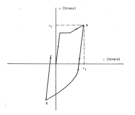
Then Aktan et al. (1973) described the stress-strain relationship for each half-cycle between two stress-reversals using the Ramberg-Osgood function, illustrated in Figure 1.5, defined in Eq. (1.2).
0 0 0 i i i (1.2)
Where and denote the strain and stress, and i and i are the initial
values of the strain and stress at the beginning of the half cycle. 0 and
0
are the yield strain and yield stress, and is the parameter of the Ramberg-Osgood function.
Figure 1.5 Cyclic model proposed by Aktan et al. (1973) based on Ramberg-Osgood Model
Ma, Bertero, and Popov (1976) divided each half cycle into elastic, plastic and hardening periods, and proposed a series of rules to describe the cyclic unloading and reloading stress-strain relationship respectively, based on the Ramberg-Osgood model, as shown in Figure 1.6.
b) Reloading curve of the second reversal and subsequent half cycles Figure 1.6 Cyclic model for rebar proposed by Ma et al. (1976) based on
Ramberg-Osgood model
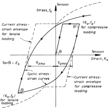
Thompson and Park (1978) proposed the cyclic model adopting the Ramberg-Osgood model with empirical constants to describe the cyclic stress-strain relationship. As shown in Figure 1.7, the stress-strain curve for monotonic loading, with suitably adjusted origin of co-ordinates, is used to describe the envelope which the steel stress cannot exceed.
Figure 1.7 Cyclic stress-strain curve with envelope proposed by Thompson and Park (1978) based on Ramberg-Osgood model
On the contrary, in the explicit algebraic model, the strain is the independent variable, and the corresponding stress is the dependent variable.
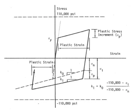
One multiline model was proposed by Aktan et al. (1973) to simulate the cyclic behaviors including isotropic hardening. The initial stress-strain relationship is elastic-plastic with strain hardening slope. If any plastic strain is obtained for the half cycle before the reversal, the boundary of the hardening line will shift against the horizontal axial. Meanwhile, the slope of the hardening line is less than the slope of the previous hardening line, as illustrated in Figure 1.8.
Figure 1.8 Cyclic stress-strain curve with envelope proposed by Aktan et al. (1973)
Then Aktan and Ersoy (1980) suggested another multiline model to describe the cyclic behaviors of reinforcing bars considering the Bauschinger Effect, illustrated in Figure 1.9.
Menegotto and Pinto (1973) built up a widely applied explicit model which was first proposed by Giuffre and Pinto (1970). The stress-strain relationship is defined by Eq. (1.3):
* * * 1 * ( 1 ) = b ( 1 R )R b (1.3)
where b is the hardening ratio between the tangent modulus of the
asymptote after yielding point and the initial tangent modulus at the original point or reversal point, defined in Eq. (1.4); the normalized stress
*
and strain *are defined in Eq. (1.5); the curved transition from the
initial asymptote with initial tangent modulus E0 to the hardening
asymptote with slope equal to bE is defined by R in Eq. (1.6). 0
0 b Es E (1.4) * 1 n r n n y r and * 1 n r n n y r (1.5) n r and n r
are the strain and stress corresponding to the reversal point which is the intersection between the nth half cycle and n+1 half cycle.
1
n y
and n 1
y
are the stain and stress corresponding to the yield point of
the n+1 half cycle. The yield point is the intersection of the asymptotes which are the envelope of the n+1 half cycle. The asymptote at the reversal point is determined by the reversal point ( n
r
, n r
) and the unloading slope ratioE . Subsequently, the yield stress 0 yn1 could be
determined by the yield stresses 1 y
andyn , strains
y
n
and rn and
hardening ratio b. Then n 1
y could be obtained by n r , n 1 y and tangent
modulusE . Hereby the second asymptote could be determined by the 0
yield point and the hardening ratio b.
1 1 0 2 n n n A R R A (1.6)
In Eq. (1.6), n is the plastic excursion at the nth semi cycle normalized by
the strain y corresponding to the initial yield stress f , defined as: y
n n
n r y y
; R is the initial curvature value, 0 A and 1 A are the 2
constant parameters depending on the material properties. The greater the value of R , the steeper the transition curve.
Figure 1.10 Menegotto-Pinto Model
The typical cyclic stress-strain curve depicted by the Menegotto-Pinto model is shown in Figure 1.10. For the first half cycle from the origin, the yield point is A, the curve transition parameter R equals R0 . At the reversal B, the
asymptote (2) is determined and thus the yield point of the unloading half cycle is obtained which is the intersection C of the asymptote (2) and (3). The curve transition parameter R is calculated according to 1 1 the plastic
excursion of the last half cycle. Likewise, the yield point F and the curve transition parameter R are determined at the reversal point D. 2
Stanton and McNiven (1979) compared the Ramberg-Osgood model and the Menegotto-Pinto model and pointed out that the Menegotto-Pinto demonstrated advantages over the Ramberge-Osgood model. The Menegotto-Pinto model could generate numerical curve with more
computional efficiency and smaller minimum error. The authors pointed out that the second envelope in the original Menegotto-Pinto model, which is a straightline and is definitely not the real dynamic envelope of the typical steel, should be replaced by monotonic skeleton curve. Furthermore, the authors studied the effect of the strain hardening on the cyclic stress-strain relationship of the rebar and proposed one function to calculate the stress shift at each reversal, in Figure 1.11.
Figure 1.11 Modified Menegotto-Pinto model by Stanton and McNiven (1979)
Filippou, Bertero and Popov (1983) thought that the original Menegotto-Pinto Model could simulate the real stress-strain relationship accurately enough if the strain hardening is considered properly. The authors put forward Eq. (1.7) to calculate the stress shift due to isotropic hardening.
3 max 4
st ya y a
(1.7)
Where max is the absolute maximum value at the reversal of previous half cycles, y and y, respectively, are the yield strain and yield stress, and a and 3 a are the experimentally determined parameters. 4
Dodd and Restrepo (Dodd & Restrepo-Posada, 1995) built one model for the cyclic behaviors of carbon steel rebar without buckling and proposed the empirical formulas for updating the tangent modulus at reversal in
tension and compression respectively, which could be used to modify the Menegotto-Pinto model.
1.2.2 Steel Model Incorporating Inelastic Buckling
Monti and Nuti (1992) proposed the first model which could consider the buckling of the reinforcement based on a series of experimental tests on carbon steel rebar. The authors proposed a series of rules to consider the effects of strain hardening on the yield stress and hardening ratio between the second asymptote and the first asymptote.
The Monti-Nuti model is proposed based on the experimental observation of carbon steel rebar Feb44 with yield stress 450 MPa which was produced in Italy. The effect of the yield stress of different types of rebar is not considered properly in the model.
Gomes and Appleton (1997) built up one model describing the monotonic compressive skeleton curve based on the equilibrium of plastic mechanism of a buckled rebar. The authors describe the buckled compressive branch with the proposed model and simulate the tensile branch and the unbuckled compressive branch with the Menegotto-Pinto model. The combined model is illustrated in Figure 1.12.
Figure 1.12 Combination of Gomes and Appleton Model and Menegotto-Pinto Model
The Gomes-Appleton Model is set up based on the equilibrium equation of fix-ended column and assumption that the plastic hinge occurs in the midspan of the column. This model doesn’t consider the effect of cyclic loading and unloading on the yield stress variation.
Dhakal and Maekawa (2002b) suggested the monotonic skeleton curves of reinforcement in tension and compression, respectively, shown in Figure 1.13. Also the authors presented formulas to update the tangent modulus at the reversal points in tension and compression, respectively. Then the parameter b in the Menegetto-Pinto model is modified and the skeleton curves are applied to describe the stress-strain relationship when the strain exceeds the attained maximum or minimum strain of previous half cycles. This model doesn’t consider the yield stress variation at the reversal.
b) Monotonic compressive skeleton curve
Figure 1.13 Monotonic Skeleton curve proposed by Dhakal and Maekawa(2002b)
Kunnath, Heo, and Mohle (2009) developed the combined material model in OpenSees named as “ReinforcingSteel” based on the Chang and Mander (1994) uniaxial steel model incorporating Gomes-Appleton model and Dhakal-Maekawa model.
Zong (2010) proposed the “beam on spring” model to simulate the stiffness of the confinement from the transverse stirrups, as illustrated in Figure 1.14, and then the model was simplified into trilinear model to adopt the “Hysteretic” material model in OpenSees, shown in Figure 1.15. The formulas in the model are empirical formulas derived through data fitting on a series of numerical data generated by the 3D FEM model of the rebar.
Figure 1.14 Schematic Diagram of rebar in Concrete Column
b) proposed model application in OpenSees Figure 1.15 Trilinear Model proposed by Zong (2010)
1.3 SIGNIFICANCE AND AIMS OF CURRENT
RESEARCH
The proper steel material model for rebar incorporating buckling is crucial for the seismic analysis of the reinforced concrete structures. In this paper, the modified Monti-Nuti model is proposed and the effectiveness is demonstrated.
1.3.1 Significance
As introduced above, evaluation of the seismic performance of existing reinforced concrete structures is important to ensure the inhabitants and property safe in case of earthquake. The accurate cyclic model for rebar incorporating inelastic buckling is very important for seismic analysis of the concrete structures (Bae, Mieses, & Bayrak, 2005).
In this study, cyclic behaviors of different types of rebar are carefully researched and one improved Monti-Nuti model for rebar is proposed.
This model solves the drawbacks of existing model and could obtain more accurate result with less computational cost.
1.3.2 Aims of Current Research
In this thesis, one modified Monti-Nuti model is proposed to simulate the cyclic behaviors of rebar such as carbon steel rebar and stainless steel rebar, based on the experimental and numerical study of carbon steel rebar and stainless steel rebar.
The parameters in the modified Monti-Nuti model are identified by the Genetic Algorithm. The effectiveness and robustness of the parameters are verified.
The modified material model is implemented in the OpenSees, and the material model is named as “Steel05”.
The numerical curves generated by the modified model are calibrated with the experimental curves.
The material model is applied in the structural analysis of cantilever column.
Finally, the effect of corrosion of rebar on the cyclic stress-strain behavior is studied and the corrosion extend model is proposed.
1.4 Organization of this Thesis
In section 2, the essence of the original Monti-Nuti model is explained in detail. In section 3, the drawbacks of the original model are studied and then the improved Monti-Nuti is proposed. In section 4, the parameters in the model are identified by the Genetic Algorithm and the formulas for the parameters are proposed. In section 5, the implementation of the material in OpenSees is briefly introduced, and the numerical model is validated with the experimental curves. In section 6, the application of the modified Monti-Nuti model in reinforced concrete piers is made to verify the effectiveness of the new material model. In section 7, the effects of corrosion of rebar are studied and the corrosion extended model is proposed. Finally in section 8, main conclusions and the further work are briefly discussed.
2. ORIGINAL MONTI-NUTI MODEL
The Monti-Nuti Model is proposed based on experimental observation of the carbon steel rebar (Giorgio Monti & Nuti, 1992). This model consists of four hardening rules such as kinematic rule, isotropic rule, memory rule and saturation rule. The model calculates the yield stress, elastic modulus, hardening ratio and the curve transition parameter at each reversal, which considers the effects of strain hardening in absence of buckling and in presence of buckling respectively.
2.1 MONOTONIC SKELETON CURVE
A series of experiments on carbon steel rebars Feb44, with yield stress equal to 450 MPa, diameter D=16, 20, 24 mm, were tested under monotonic tensile, compressive and cyclic loads, and the monotonic curves are illustrated in Figure 2.1.
Figure 2.1 Monotonic tests of carbon steel rebar (Giorgio Monti & Nuti, 1992)
Several observations could be obtained in Figure 2.1. 1) the tensile monotonic curves are identical regardless of the slenderness of the rebar; 2) even though the diameters of the rebars are different, the monotonic compressive could be identical if the slenderness ratios L/D are equal; 3) when the slenderness ratio L/D equals 5, the monotonic compressive curve coincides with the monotonic tensile curve; 4) when the slenderness ratio L D is 11, the monotonic compressive curve diverges from the
tensile curve as soon as it reaches the yield point; 5) when the slenderness ratio L D varies between 5 and 11, the compressive curve coincides with
the tensile curve for certain length, and then the compressive curve diverges from the tensile curve.
The skeleton curve for the rebar in the Monti-Nuti model is shown in Figure 2.2. The skeleton curve in tension is a bilinear curve. As shown in Figure 2.2 a), the slope of the first line is the initial tangent modulusE , after the stress 0
exceeds the yield stress 0
y
, the curve converts to the second line with slope equal to bE , where 0 bis the hardening ratio.
The monotonic compressive skeleton is shown in Figure 2.2 b). After the stress reaches the yield point A, the path for the curve dependting on the slenderness ratio L D:
The curve converts to the line (1) with the slope ratio equal tob E0 0, where
0
b is positive and equals the hardening ratio in the tensile curve, if the
slenderness ratioL D5;
The curve converts to the line (2) with the slope ratiob E0 0, where b0is
negative representing the hardening ratio in compression, if the slenderness ratio L D11;
The curve follows the line (1) for lenth s until point B, and then swiths to line (3) with slope ratio b E0 0, if the slenerness ratio 5 L D11.
A 0 str e ss ( M P a ) strain (%) A: yield point E0 b*E0
y0 0 b: hardening ratio E0: initial elastic modulusa)Tensile skeleton curve
b) Compressive skeleton curve
Figure 2.2 Monotonic skeleton curve of Monti-Nuti model
s
is the superposition length between the monotonic tensile curve and the monotonic compressive curve after the yield point, and the formula is given in Eq. (2.1) based on the experimental observation.
( 5 ) 11 0 5 L 11 1 s c L D L D for D e (2.1)
c is a parameter related to the rebar, and the given as 0.5 in the test.
2.2 HARDENING RULES FOR CYCLIC
BEHAVIORS OF STEEL REBAR
As mentioned above, the effect of strain hardening on the cyclic behaviors of stress-strain curves should be considered properly if the Menegotto-Pinto Model is adopted to simulate the cyclic behaviors of reinforcing bar. The Monti-Nuti model could update the yield stress of each half cycle and the hardening ratio between the hardening modulus and the initial elastic modulus.
The stress variation is calculated by equations incorporating the strain hardening which represents the plastic deformation of the rebar after exceeding the yielding point. If an isotropic specimen under tension or compression is loaded exceeding the yield strength, and then it is unloaded and reloaded towards the opposite direction, the yield strength will become smaller or larger due to the plastic deformation at pervious loading process. The effect of the plastic deformation could be divided into kinematic hardening and isotropic hardening.
According to the experimental results, the critical slenderness L D
equals 5, where L is the distance between the subsequent transversal rebars and D is the diameter of the longitudinal rebars. If the slenderness
L D exceeds 5, the buckling could be observed in the experimental stress-strain curves, otherwise, no buckling occurs. The effects of strain hardening in absence of buckling and in presence of buckling are different.
2.2.1 In Absence of Buckling
The kinematic hardening results in the yield stress reduction in the opposite direction after the specimen is loaded exceeding the yield strength in tension or compression. The kinematic hardening could explain the Bauschinger Effect. This kinematic hardening is considered in the original Menegotto-Pinto model. In Figure 2.3 a), the yield stress
corresponding to point C is smaller than that of point A due to the 1 kinematic strain hardening 1
p
. Meanwhile, the yield stress corresponding to point F is 2 smaller than the enlarged yield stress corresponding to point B in tension, due to the kinematic strain hardening 2
p
in the second half cycle. In one word, the effect of the kinematic is to pull the yield strength towards the horizontal axis.
a) Effect of kinematic hardening
b) Effect of isotropic hardening
On the contrary, the isotropic strain hardening causes the yield stress to increase in the opposite direction. As shown in Figure 2.3 b), the isotropic strain hardening 1
p
causes the yield point in the second half cycle to move from C1 to C2. Likewise, the isotropic strain hardening p2 results in
the shift of the yield point from F1 to F2. However the isotropic hardening will have no effect on the stress variation if the absolute value of the plastic deformation (like 2
p
) doesn’t exceed the absolute value of the maximum plastic deformation of previous half cycles (likemax). This means that the isotropic hardening has the memory character which decides that the isotropic hardening only take effect when the current strain hardening is beyond the maximum previous plastic strain deformation. Different from the effect of the kinematic hardening, the effect of the isotropic hardening is to transfer the yield point away from the horizontal axis.
A half cycle is the path between two subsequent load reversals. The plastic excursion at the nth half cycle is defined in Eq. (2.2):
(n 1,2,3, ) n n n p r y (2.2) where n r
is the strain corresponding to the reversal point at the end of the nth half cycle and n
y
is the strain corresponding to the yielding point which is the intersect of the two envelope lines at the nth half cycle, and is calculated according to Eq. (2.3).
1 1 (n 2,3,4, ) n n y r n n y r E (2.3) where n y
is the yield stress of the nth half cycle, n 1
r
is the stress
corresponding to the end reversal point of the n 1 half cycle. Then the half cycle plastic work n
p
decides the sign of the stress variation and is defined as follows, in Eq. (2.4):
1 2 n n n n p r y p (2.4)The hardening ratio b is always positive both in tension and in
stress reduces with the strain decreasing. Thereby the plastic work n p
is
always positive in absence of buckling. 1. Kinematic rule
The kinematic rule corresponds to the effect of the kinematic strain hardening. The stress variation due to the kinematic rule is given in Eq. (2.5): 1 n n i K p i bE
(2.5)For each half cycle, the stress variation i p
bE reduces the absolute value
of the yield stress in the opposite direction. 2. Isotropic rule
The isotropic rule corresponds to the effect of the isotropic strain hardening. The stress variation due to the isotropic rule is defined in Eq. (2.6):
1 sign( ) -n n i n n I p p p i bE sign
(2.6)where sign(x) is the sign function: sign(x) 1 if x 0 ;sign(x) if 1
x 0 ; otherwise sign(x) 0 .
The stress variation due to the isotropic rule is always opposite to the strain variation of current half cycle, thus it will always increase the yield stress in the opposite direction.
3. Memory rule
According to the experimental results, if the plastic excursion at current half cycle n
p
doesn’t exceed the maximum plastic excursion of the previous n1 half cyclespmax, no isotropic hardening develops at current
half cycle. Thus one new symbol n p
is defined in Eq. (2.7) to describe this character.
maxn n n
p p p sign p
(2.7)
where u uH u
is the step function. If u0, H u
1; otherwise,
0H u . Replace pi in Eq. (10) with ip in Eq. (11), the stress variation
due to the isotropic rule and memory rule is named as n IM and is defined in Eq. (2.8):
1 n n i i n IM p p p i bE sign sign
(2.8)The yield stress at the n+1th half cycle could be calculated by Eq. (2.9):
1 1 1
n n n n
y ysign p P K P IM
(2.9)
where P is the weight coefficient which determines the contribution made by the kinematic rule and the isotropic rule. The value of P depends on the properties of the material. In the experimental tests on the carbon steel rebar, P is given as 0.5 (Giorgio Monti & Nuti, 1992).
2.2.2 In Presence of Buckling
Due to buckling, the absolute value of the stress in compression decreases with the strain increasing after the unloading path exceeds the yield point. Hereby the effects of the kinematic hardening and isotropic hardening are different from that in absence of buckling.
a) Effect of kinematic hardening
b) Effect of isotropic hardening
Figure 2.4 Effect of strain hardening in presence of buckling
As shown in Figure 2.4 a), the effects of the kinematic hardening are different in tension and compression. The strain hardening in tension could cause the absolute value of the yield stress reduction in compression. The absolute value of the stress corresponding to point C is
smaller than the yield stress of point A. However, the strain hardening in compression increases the yield stress in tension (The yield point shifts from F1 to F2). Like the isotropic hardening rule in absence of buckling, the kinematic hardening will have no effect if the absolute value of the plastic hardening of current half cycle doesn’t exceed the maximum plastic deformation of previous half cycles (for instance, if 2
max
p
, the stress variation =0), which means that the kinematic hardening has 2 the memory character in presence of buckling. In general terms, the effect of the kinematic hardening is to move the cyclic curve upwards in presence of buckling.
In Figure 2.4 b), the isotropic hardening will increase the absolute value of the yield stress in compression but reduce the yield stress in tension. In one word, the effect of the isotropic hardening is to shift the cyclic curve downwards (Move the yield point C1 to C2 and shift the yield point F1 to F2.).
In presence of buckling, the half cycle plastic work n p
is still positive in tension, but it becomes negative in compression due to the stress increase with the strain decreasing as the hardening ratio b is negative in
compression. Thus the rules corresponding to the kinematic strain hardening and isotropic hardening in presence of buckling are different from those in absence of buckling.
1. Kinematic rule and Memory rule
The stress variation due to the kinematic rule will not develop if the plastic excursion at current half cycle n
p
doesn’t exceed the maximum plastic excursion of the previous n-1 half cycles max
p
. Thus, the stress variation is calculated via the combination of the kinematic rule and the memory rule, and is given in Eq. (2.10):
1 n n i KM ,b p i bE
(2.10)In tension, the hardening ratioband the additional plastic excursion ip
are positive, thus i p
bE is positive, and then the absolute value of the
ratioband the additional plastic excursion ip are negative, thus bEip is
positive, which will result in the increase of the yield stress in tension. 2. Isotropic rule
The expression of stress variation is the same with that defined in absence of buckling. However, the effect of the isotropic rule is different. In tension the plastic work n
p
is positive, thus the absolute value of the yield stress in compression will increase. In compression, the plastic work
n p
is negative; as a result, the yield stress in tension will decrease. The yield stress at the n+1th half branch could be calculated according to the Eq. (2.11):
1 1 1 n n n n y ysign p P KM ,b P I (2.11) 3. Stress shiftIf the slenderness ratio 5 L D11 , as shown in Figure 2.5, the
superposition lengthswill be positive, thus the intersection between the two asymptotes will shift from the original yield point A to another position B. In order to eliminate the discontinuity, the shifted yield stress could be calculated according to Eq. (2.12), which is deduced based on geometrical considerations. 1 sh s b b E b (2.12)
Where E is the tangent modulus at the original point of the unloading half cycle, bis the hardening ratio of the superposition zone, bis the slope of the buckled asymptote, which is negative.
Figure 2.5 Stress shift in compressive curve
2.3 CURVE TRANSITION PARAMETER R
The curve transition parameter R defines the curvature of the transition from the first asymptote to the second envelope. The larger the value of R , the steeper the curve transition. In Figure 2.6, R >0 R
1 >R
2 , theFigure 2.6 Degradation of curve transition
In Monti-Nuti model, the parameters in the expression for R is redefined in absence of buckling and in presence of buckling, respectively.
2.3.1 In Absence of Buckling
Different from the original equation, the formula for the curve transition
R is defined in Eq. (2.13): 1 max 1 0 2 max n A R R A (2.13)
Where max is the maximum plastic excursion, defined as
max max( )
n p
. Through calibration, R is set 20, 0 A equals 18.5 and 1
2
A is 0.0001.
2.3.2 In Presence of Buckling
The parameters A and1 A in the formula corresponding to R , are 2
modified according to the calibration of the experimental results, and the formula is given in Eq. (2.14).
1 max 1 0 1 2 max b b b n b A R R R A (2.14)
where max is the maximum plastic excursion, defined as
max max( )
n p
, 1b
A =19.5, A =0.001, 2b R is defined in Eq. (2.15) and 0b
the lower boundary 1b
R is defined in Eq. (2.16).
0 0 2 b cr R R L D L D (2.15)
1 10 b cr R L D L D b (2.16)2.4 HARDENING RATIO
b represents the ratio between the hardening modulus and the initial
elastic modulus at the reversal point. In Figure 2.7, the effect of b on the
curve is illustrated. If b>0, the stress increase with the increase of strain
after the yield point; if b<0, the stress reduce with increase of strain after
the yield point.
a) b=0; b) b>0; c) b<0