Paolo Liberati, Giuliano Resce,
Francesca Tosi
The probability of multidimensional
poverty in the European Union
Dipartimento di Scienze Statistiche “Paolo Fortunati”
Quaderni di Dipartimento
Serie Ricerche 2020, n. 1
ISSN 1973-9346
The probability of multidimensional poverty in the European
Union
Paolo Liberati
Department of Economics, Roma Tre University, [email protected]
Giuliano Resce
Italian National Research Council, [email protected]
Francesca Tosi
Department of Statistical Sciences “Paolo Fortunati”, University of Bologna, [email protected]
Abstract. This paper evaluates multidimensional poverty in European countries introducing two main novelties compared with the previous literature: first, the dimensions of poverty are selected on the basis of the shared values included in the Charter of Fundamental Rights of the European Union; second, the whole space of feasible weights is used to summarise the multidimensional information, in order to remain agnostic about the importance given to the different deprivations. Using data from four waves of EU-SILC, the methodological innovations introduced here have allowed to produce a family of measures that capture the individual probability of being multidimensionally poor. Individual probabilities are then used to analyse the within and between distribution of multidimensional poverty in ten countries. Finally, they get combined with the generalised Lorenz dominance techniques in order to derive socially preferred distributions with the minimum load of value judgments. The novel methods proposed in this analysis allow to move from a dual definition of poverty, where poor and non-poor individuals are classified in a mutually exclusive context, to a continuous measure of deprivation, which allows to capture both the extensive and intensive margin of multidimensional poverty.
Keywords: Multidimensional Poverty; Charter of Fundamental Rights; Hierarchy Stochastic Multicriteria Acceptability Analysis; Povertà multidimensionale, Carta dei Diritti Fondamentali; Analisi Stocastica di Accettabilità Multicriterio
1. Introduction
There is widespread agreement on the need to conceptualise poverty as a multidimensional phenomenon. Low consumption or income is surely at the heart of the notion of poverty but several other domains, like poor human health, limited access to education and powerlessness, are systematically concerned by inadequate living standards (Ferreira and Lugo, 2013).
Since the pioneering works of Tsui (2002) and Bourguignon and Chakravarty (2003), a number of approaches were developed to measure deprivation in multiple dimensions (see among others Alkire and Foster, 2011; Chakravarty et al., 1998; Cheli and Lemmi, 1995; Chiappero-Martinetti, 1994; Deutsch and Silber, 2005; Maasoumi and Lugo, 2008). However, multidimensional poverty measures are far from being universally welcomed. One of the main debates around them concerns the degree of arbitrariness used to define suitable dimensions and indicators of poverty, to set poverty thresholds, and to specify a system of weights to aggregate the various dimensions.
To begin with, which dimensions matter and who should be selecting them are questions that repeatedly raise issues of ethics and legitimacy. The method most used for selecting dimensions is drawing on a list generated by public consensus.1 However, retrieving information on shared societal values is not
straightforward when the analysis is carried out at international or even at the global level (Alkire, 2007). The identification of deprivation indicators and poverty thresholds – to be set both within and across indicators – requires further sensitive decisions, although they end up being data-driven in most cases, especially when the poverty analysis is performed in the ‘counting of deprivations’ framework (Alkire et al., 2015).
Relative weights attached to attributes of different nature are also a matter of concern. In the income-centred framework, prices are commonly used to aggregate components of consumption expenditure (or the incomes used to finance such consumption). They are then used to compose an index of aggregate consumption to be compared with an aggregate poverty line defined in the same space. Ideally, such an aggregation includes not only market goods and services, but also imputed values for non-market commodities, like public goods (Ravallion, 2011). Even though there exist different reasons why prices might not be ideal welfare weights2,
they provide a clear understanding of the effects of the weighting scheme (Maasoumi and Lugo, 2008) as they explicitly address the issue of trade-offs between different goods and services, or the rate at which consumers are willing to trade one unit of an expenditure component for another (i.e., the marginal rate of substitution – MRS – between two goods). Moreover, MRSs play the important role of informing on whether two commodities, for every individual, are complementary, independent or substitutes – that is, whether, if we increase the quantity of one good, the final utility of the other increases, remains constant or decreases (Schultz, 1935).
1 See for instance the Sustainable Development Goals experience (Fukuda-Parr, 2016).
2 Among these: (i) the existence of externalities and missing or highly imperfect markets; (ii) the fact that price data are often
geographically coarse, so actual price variation in space is missing from the information available to the researcher; and (iii) the regular need for imputing prices for market as well as for non-market goods (Bourguignon and Chakravarty, 2003; Ferreira and Lugo, 2013).
Similarly, in a multidimensional setting relative weights play the central role of determining trade-offs between dimensions. They reflect value judgments and possibly the very structure of social preferences. For these reasons, the setting of a weighting system is inevitably subject to the formulation of strong normative assumptions and ethical considerations on what a ‘good life’ is, and should be made as explicitly as possible.
The literature provides an array of methods – normative, statistical, or hybrid – to set relative weights in a multidimensional context (Decancq and Lugo, 2013), although in practice, because well-being dimensions are deemed equally important from an ethical point of view, weights are often distributed equally among dimensions, as in the case of the Human Development Index (UNDP, 1990). Moreover, quantifying how many units of, say, education an individual would give up to compensate one extra year of life is a rather complicated task. In the first place, such an evaluation would require an amount of information that might not be easy or possible to retrieve. Second, the MRS between any two dimensions – that is, the amount of the first dimension that an individual is willing to give up for the second one while maintaining the same level of well-being (Decancq and Lugo, 2013) – could vary from an individual to another on the basis of the actual levels of the considered achievements, as in the case of age.
This has relevant implications whenever one wants to compare not only individuals but also different territorial entities, like European Union (EU) countries. Empirically, assuming one specific vector of weights to be attached to a given set of dimensions may heavily affect both interpersonal comparisons and country rankings (Foster et al., 2013), leading to less robust results.
This paper shows that it is possible to minimize the degree of arbitrariness commonly used to choose dimensions and weights in order to compare selected EU countries on the basis of a multidimensional poverty index. To this purpose, it first employs a normative approach to derive relevant dimensions from an expression of public consensus, that is the Charter of Fundamental Rights of the European Union (European Parliament, Council of the European Union, and European Commission, 2000). Then, drawing on the data on income and living conditions in the EU made available by Eurostat (EU-SILC), it addresses the issue of weighting dimensions by applying Stochastic Multicriteria Acceptability Analysis (SMAA) (Lahdelma and Salminen, 2001), which allows to embody unknown preferences on the weights assigned to each dimension. Such an approach was previously used to investigate health outcomes, both in Italy and the US (Lagravinese et al., 2019a, 2019b). In this article, SMAA techniques are used for the first time to construct a robust composite poverty index based on individual-level data for all feasible sets of weights.
The article is organised as follows: in Section 2, the identification strategy to select the various dimension of poverty in EU countries is discussed, along with the choice of deprivation indicators and poverty thresholds. Section 3 introduces the SMAA methodology, while Section 4 presents the results from both a cross-country and a diachronic perspective, and analyses the overall inequality in the distribution of the probability of being multi-dimensionally poor, within and between countries, according to the Analysis of Gini (ANOGI) methodology (Liberati, 2015), adapted to a multidimensional setting as proposed by Lagravinese et al. (2019a). Finally, in Section 5 the Generalised Lorenz dominance technique is used to perform pairwise country
comparisons of the distribution of probabilities to rank them from a social perspective with the minimum load of value judgments. Section 6 concludes.
2. Assessing multidimensional poverty in the European Union
Poverty measurement implies the accomplishment of two fundamental tasks: the first is to identify the poor among the total population; the second is to aggregate the information about the poor, either through the use of a poverty index (Sen, 1976) or by using dominance ordering (see, for example, Deaton, 1997). When performed in a multidimensional setting, the identification step requires to make several choices, including defining suitable dimensions and indicators, setting poverty thresholds whenever appropriate, and defining a system of weights.
The information about the poor can be then aggregated either first across individuals and then across dimensions (e.g. the HPI, Anand and Sen, 1997), or first across dimensions and then across individuals (e.g. the Global MPI, Alkire and Santos, 2014). Each type of aggregation order has empirical advantages and disadvantages. Aggregating first across dimensions and then across people typically imposes a restricted choice of the usable data, which has to come from the same source for the studied population. Yet, poverty measures based on this kind of aggregation are very appealing as they are able to account for people’s simultaneous deprivations in different spheres of life.
In the context of the EU, such kind of statistical source is represented by the European Union Statistics on Income and Living Conditions (EU-SILC), which was launched in 2003 on the basis of an agreement between Eurostat and a number of Member States with the aim of providing timely and comparable annual data on variables such as income, social exclusion, material deprivation, health, education and labour at both household and individual level. Although the EU-SILC does not cover all the domains that could be of interest for a multidimensional poverty analysis, it is still wide enough to assess deprivations over multiple facets of life. Moreover, since 2010 it is also used for monitoring poverty and social exclusion in the EU in accordance with the Europe 2020 Strategy, reason why it appears to be an appropriate and sound basis of information to measure multidimensional poverty in the EU.
2.1 Dimensions selection
In order to produce reliable statistics, procedures for selecting life domains in a multidimensional setting should minimize the degree of arbitrariness. Alkire (2007) suggests different methods to select poverty dimensions, summarized in five main processes: (i) relying on existing data or convention; (ii) making normative assumptions; (iii) drawing on a list generated by consensus; (iv) using an ongoing deliberative participatory process; (v) using empirical evidence regarding people’s values.
One method that is widely used within institutions at the global level is the public consensus one (see, e.g., the Human Development Index experience). As put by Alkire (2007), this method consists in identifying a set of dimensions that have been established through some consensus-building process at one point in time
and are relatively stable. In some countries, it has been used to justify the exploitation of National Constitutions and laws to retrieve information on publicly agreed values – see the National Council for Evaluation of Social Development Policy experience in Mexico (CONEVAL, 2010) and some scholarly initiatives (Burchi et al., 2014).
Retrieving information on shared societal values is however not unequivocal when it comes to a supranational entity like the EU. One possible source of such a piece of information is the Charter of Fundamental Rights of the European Union, a document containing the declaration of the common values of the peoples of Europe (European Parliament, Council of the European Union and European Commission, 2000). The Charter was incorporated into the Treaty of Lisbon in 2009 and has since then come into legal force in Member States. It conveys a shared understanding of social justice and states the principles according to which the Union commits itself to fight poverty and social exclusion. The great majority of its articles deal with the domain of civil and political liberties and different kinds of freedoms (e.g., the right to life and the protection of human dignity, the right to the integrity of the person, the prohibition of slavery, forced labor, torture and degrading treatment, the right to security of the person, the respect for private and family life, the freedom of thought, conscience and religion, the freedom of expression, assembly and association).
In addition, the Charter recalls other valuable life dimensions. The first one is decent work, or the right to employment opportunities for productive work and the possibility to deliver a fair income in conditions of freedom, equity, security and human dignity (ILO, 1999). Social solidarity appears as another possible dimension to value, which includes the right to the provision of social and economic protection, for instance through the access to services of general economic interest, consumer protection, the entitlement to social security benefits in the case of loss of employment, maternity, illness, dependency or old age and through the right to property. Finally, the broader concept of human development – or the right to the human flourishing of individuals in a just and protected environment – emerges from the Charter, through the right of education, the freedom of arts and sciences, the protection of human health and the environment.
Even though it might not be considered as definitive, we start from this list of dimensions (summarized in Table 1) as a base of shared societal values to be used to inform the multidimensional assessment of poverty for EU countries.
2.2. Deprivation indicators
Regarding the choice of the indicators, the EU-SILC does not cover all the dimensions identified by the Charter. Variables accounting for the first dimension, Political and civil liberties, are completely missing in the database, the reason why this dimension will not be considered in the following analysis.3
For the Decent work dimension, we follow the review of EU-SILC labour-related indicators provided in Tosi (2015) to select two relevant indicators: Activity status (PX050) and Low work intensity (RX050),
3 Acknowledging that it is not possible to retrieve in the data all the information that is considered theoretically essential does not
constitute a shortcoming of the proposed approach. As also recommended by Robeyns (2003), an explicit and openly discussed selection of suitable life domains is a step that needs to be performed before endeavoring any kind of empirical assessment, so as to avoid relying only upon the available information and, possibly, to stimulate a more specifically targeted data collection.
respectively accounting for employment conditions and (quasi-) joblessness, as conceived by Eurostat as part of the composite indicator At Risk of Poverty and Social Exclusion rate (AROPE).
Regarding the Social solidarity dimension, different indicators in the EU-SILC allow to capture the level of social protection offered to European citizens, e.g., through the variables Family/Children related allowances, Social exclusion not elsewhere classified, and Housing allowances. In fact, because all the policies just mentioned sustain people’s standard of living by integrating their income through the channel of monetary transfers, it appears reasonable to choose an income poverty indicator as a general proxy for this dimension. The variable Monetary poverty (after transfers) (HX080) is thus used to account for deprivations in the Social solidarity dimension.
Finally, in the EU-SILC there are different variables that can be used to construct deprivation indicators in the last dimension, Human development. Some of them relate to human health, while some others refer to the educational attainment or to the quality of the living environment. The nine selected variables and the corresponding modalities are extensively commented in Tosi (2015) and outlined, along with all the chosen indicators, in Table 2.
Table 1 – An application of the overlapping consensus method to the Charter of Fundamental Rights of the European Union
Dimension Values and principles Articles of the Charter
POLITICAL AND CIVIL
LIBERTIES Human dignity, Right to life, Right to the integrity of the person, Prohibition of torture, slavery and forced labour, Right to security, Protection of personal data, Respect for private life and the right to marry, Freedom of thought, conscience and religion, Freedom of expression, assembly and association, Freedom of the arts and sciences, Right to asylum, Protection in the event of removal, expulsion or extradition, Equality before the law, Right to non-discrimination, Protection of cultural, religious and linguistic diversity, Right to vote and to stand as a candidate at elections, Right to good administration, Right to petition, Freedom of movement and residence, Right to a fair trial, Presumption of innocence and right of defence
1–13, 18–22, 39–50
DECENT WORK Freedom to choose an occupation and right to engage in work,
Equality of employment, work and pay for women and men, Right to information and consultation within the undertaking, Right of collective bargaining and action, Right of access to placement services, Protection in the event of unjustified dismissal, Fair and just working conditions, Prohibition of child labour, Protection from dismissal for a reason connected with maternity and right to parental leave
15, 23, 27–33
SOCIAL SOLIDARITY Freedom to conduct a business, Right to property, Social, economic and legal protection of the family, Right to social security and social assistance, Integration of persons with disabilities, Health care and protection, Access to services of general economic interest, Consumer protection
16, 17, 26, 33, 34, 35, 36, 38
HUMAN DEVELOPMENT Freedom of the arts and sciences, Right to education, Health care and protection, Rights of the child, Rights of the elderly, Environmental protection
13, 14, 24, 25, 35, 37
Note: Articles 13, 33 and 35 fall in more than one dimension. Source: Authors
Table 2 – Identification strategy for a multidimensional poverty assessment in the EU Dimensions Indicators Variables Cut-offs
DECENT
WORK Unemployment Activity status (PX050) 2=Employee 3=Employed persons except employees 4=Other employed 5=Unemployed 6=Retired 7=Inactive 8=Other Low work
intensity Low work intensity (RX050) 0=No low work intensity 1=Low work intensity
2=Not applicable SOCIAL
SOLIDARITY
Income poverty
Monetary poverty (HX080) 0=when HX090 >= at risk of poverty threshold (60% of Median HX090)
1=when HX090 < at risk of poverty threshold (60% of Median HX090) HUMAN DEVELOPMENT Low educational attainment
Highest ISCED level attained (PE040)
0=Pre-primary education 1=Primary education
2=Lower secondary education 3=Upper secondary education 4=Post-secondary education
5=First stage of tertiary education (not leading directly to an advanced research qualification)
6=Second stage of tertiary education (leading to an advanced research qualification)
Bad
self-reported health General health (PH010) 1=Very good 2=Good 3=Fair
4=Bad 5=Very Bad
Chronic illness Suffers from chronic illness
or condition (PH020) 1=Yes 2=No Unmet medical
needs Unmet medical need for medical examination or treatment (PH040) +
Main reason for unmet medical need (PH050)
1=Yes, there was at least one occasion when the person really needed examination or treatment but did not
2=No, there was no occasion when the person really needed examination or treatment but did not
1=Could not afford to (too expensive)
2=Waiting list
3=Could not take time because of work, care for children or for others
4=Too far to travel/no means of transportation
5=Fear of doctor/hospital examination/treatment
6=Wanted to wait and see if problem got better on its own 7=Did not know any good doctor or specialist
8=Other Poor quality of
dwelling Leaking roof, damp walls/floor/foundation or rot in window frames/floor (HH040) 1=Yes 2=No Inadequate sanitation facilities Bath/shower in dwelling (HH080/HH081) +
Indoor flushing toilet for sole use of the household (HH090/HH091)
1=Yes, for sole use of the household 2=Yes, shared
3=No
1=Yes, for sole use of the household 2=Yes, shared
3=No
Noise Noise from the neighbours or
from the street (HS170) 1=Yes 2=No
Pollution Pollution, grime or other
environmental problems (HS180)
1=Yes
2=No
Crime Crime, violence or vandalism
in the area (HS190)
1=Yes
2=No
Modalities of the EU-SILC variables indicating deprivation are highlighted in bold. Source: Authors’ elaborations
2.3 The issue of relative weights
One powerful critique to multidimensional poverty indices concerns the second issue described above, i.e. how to aggregate the different dimensions of poverty and thus how to set the weights attached to attributes of different nature. In their thorough investigation on weights in multidimensional indices of well-being, Decancq and Lugo (2013) explain that, in order to study how small changes in the achievements of different well-being dimensions can or cannot compensate each other, one needs to look precisely at the structure of weights. To this purpose, they introduce the MRS between two dimensions !" and !# as the amount of dimension 2 an individual is willing to give up for an extra unit of dimension 1, while maintaining the same level of well-being. Formally, they define the MRS between dimensions !" and !# as:
$%&'(,'* =,-(/) ,/'" /
,-(/) ,/'*
where -(/) is the well-being index and / is the vector of achievements for all ! dimensions. In fact, there exists different approaches to set relative weights in a multidimensional poverty analysis. Decancq and Lugo (2013) distinguish three classes: data-driven, normative, and hybrid. Data-driven approaches – like frequency-based weights, statistical weights (Krishnakumar and Nadar, 2008) and most-favorable weights (Melyn and Moesen, 1991) – are a function of the distribution of the achievements in the society and are not based on value judgements about trade-offs between different life domains.
Frequency-based weights often assign an inverse relation between the frequency of deprivation in a dimension and the weight of that dimension (e.g., Deutsch and Silber, 2005). The motivation behind such a relation lies in the idea that less frequent deprivations should have a higher weight because individuals would attach a higher importance to the shortfalls in dimensions where the majority in their society do not fall short, reason why some have also interpreted such weights as the “objective measures of the subjective feelings of deprivation.” (Desai and Shah, 1988, p. 52)
Statistical weights, on the other hand, are often classified into two broad sets: multivariate statistical methods, among which the most commonly used technique is based on the Principal Component Analysis (Klasen, 2000; Noorbakhsh, 1998), and explanatory models based on the idea of the latent variable, like Factor Analysis (Noble et al., 2006), the Rasch model (Fusco and Dickens, 2008), multiple indicator and multiple causes models (MIMIC) (Di Tommaso, 2006), and structural equation models (Kuklys, 2005; Krishnakumar, 2007; Krishnakumar and Ballon, 2008).
Finally, the most-favorable weights technique, which has been widely used to set weights in well-being indices (see e.g., Despotis, 2005a, 2005b; Mahlberg and Obersteiner, 2001; Zaim et al., 2001) is a particular case of the data envelope analysis proposed by Melyn and Moesen (1991) and considers weights as individual-specific and endogenously determined, i.e., the highest relative weights are given to dimensions in which the person performs best.
Conversely, normative approaches depend on value judgements about the MRSs. Weights can either be set in an equal or unequal way, although in any case they are assigned arbitrarily, that is according to particular considerations about specific trade-offs among dimensions. Arbitrariness could be overcome by following an ‘expert opinion approach’, that is, letting experts or well-informed persons decide which particular weighting scheme to attach to different poverty attributes (see for instance Chiappero-Martinetti and von Jacobi, 2012). This latter method includes the Budget Allocation Technique (Moldan and Billharz, 1997; Chowdury and Squire, 2006; Mascherini and Hoskins, 2008), where experts are asked to distribute a budget of points to the different attributes, and the Analytic Hierarchy Process (Saaty, 1987), which compares dimensions pairwise and assigns for each round a score of importance.
Lastly, hybrid approaches, like stated preference weights (Mack and Lansley, 1985; Halleröd, 1995a, 1995b; de Kruijk and Rutten, 2007; Guio et al., 2009; Bossert et al., 2009) and hedonic weights (Schokkaert, 2007; Ferrer-i-Carbonell and Freijters, 2004; Nardo et al., 2008; Fleurbaey, 2009) are a mix of the former two. As we will see in the next section, this paper tries to overcome the arbitrary choice of the set of weights, introducing a new methodology to measure multidimensional poverty. The aim will not be that of defining a specific poverty index for each individual, but that of estimating the probability that she/he will be below a given threshold for different vectors of weights.
3. Measuring multidimensional poverty: an alternative approach
Irrespective of the way of setting relative weights, all the above-mentioned approaches (i.e. data-driven, normative, and hybrid) use a single weight vector for all units (or in the case of most-favourable weights technique, a different weight vector for each unit) to reduce multidimensionality into a composite indicator. But the uniqueness of the vector of weights does not allow to take into account that, in a differentiated society, each individual may assign a different importance to each dimension. With only one vector of weights, representativeness may be valid only for a very small portion of the population. Since weights are likely to change according to individual preferences and needs, and since a “social” vector of weights could not be unanimously agreed upon, some studies have recently proposed to take into account the whole space of feasible vectors of weights in the evaluation process (Greco et al. 2018; Lagravinese et al. 2019a, 2019b).
In particular, Stochastic Multicriteria Acceptability Analysis (SMAA) (Lahdelma and Salminen, 2001) has been shown to be the appropriate tool to make comparisons in a multidimensional framework, while remaining agnostic about the weighting schemes. This methodology has an appealing application in all cases where the individual characteristics, like poverty dimensions, have to be aggregated to obtain either social norms or rankings.
Formally, using selected indicators from EU-SILC, the set of individuals 3 (4", … , 46), where 7 = 176,518 in 2008, 7 = 178,904 in 2010, 7 = 181,864 in 2012, and 7 = 182,912 in 2014, is evaluated on three dimensions (A", … , AB): 1. Decent Work; 2. Social Solidarity; and 3. Human Development. The
composite indicator can be seen as the average of the three dimensions weighted by the weights (w) associated to each of them:
(1) C-(4D, E) = F EGAG(4D)
B
GH"
where EG reflects the importance given to the dimension I, and AG(4D) the achieved result of individual 4D for dimension I. As shown in Section 2.3, Decancq and Lugo (2013) list several procedures to set E, but as the order of importance given to different indicators is a subjective choice, one single vector of E for summarising multidimensional poverty does not exist.
3.1 Stochastic Multicriteria Acceptability Analysis
In order to embody unknown preferences on the weights assigned to each dimension and to reduce the degree of arbitrariness in aggregating dimensions, SMAA considers the probability distributions JK(E) in the set of the feasible weights L (Lahdelma and Salminen, 2001):
(2) L = {(E", . . . , EB) ∈ %PB, E
"+ . . . +EB= 1}
The set of feasible weights is a (S − 1) dimensional simplex. In the absence of knowledge about the importance given to the different dimensions, a uniform weight distribution can be assumed in the set of feasible weights L. Defining UGD as the value of dimension AG for individual 4D, from the probability distributions JV(U) on W, where W is the evaluation space (in our case the space of the values assumed by the dimension AG in X), Lahdelma and Salminen (2001) introduce a ranking function attached to the individual 4D based on counting the dimensions in which a person is deprived:
(3) Y4SZ(Z, U, E) = 1 + F [[C-(U], E) > C-(UD, E)] ]`D
where [(aYbc) = 1, and [(J4dec) = 0. Hence, the rank of individual 4D, for a given vector of weights E, is one plus how many times the weighted average of multidimensional poverty of 4D (C-(UD, E)) is dominated by the weighted average of multidimensional poverty of the other individuals (C-(U], E)). Thus, the value assumed by the variable Y4SZ(Z, U, E) in equation (3) is one plus the number of individuals that are more multidimensional poor than the individual 4D. Therefore, the lower the value of Y4SZ(Z, U, E) the higher the
poverty of the individual 4D.
Accordingly, for each individual 4D and for each value that can be taken by the three poverty dimensions
U ∈ W, SMAA computes the set of weights for which individual 4D assumes rank Y:
From equation (4), one can then compute the rank acceptability index:
(5) hDf = i JV(U)
j∈V
i JK(E)
k∈Klm(j) nEnU
Equation (5) indicates the probability that the individual 4D has the Y-th position in the ranking, hDf, which
is given by the ratio of the number of the vector of weights by which individual 4D gets rank Y to the total number of vector of weights considered.
3.2 Hierarchy Stochastic Multi-Objective Acceptability Analysis
The structure of the multidimensional poverty assessment presented in Section 2 is hierarchical: dimensions are in the first level and the different indicators are in the second level. In the SMAA context, the inclusion of a hierarchical structure has been proposed by Angilella et al. (2016) and De Matteis et al. (2018). In our poverty measure, each dimension AG ∈ X is given by the weighted sum of indicators oG'∈ pG:
(6) AG = F qG'oG'
rs
'H"
In this case, the composite index of multidimensional poverty becomes the weighted average of dimensions, which are the weighted average of EU-SILC indicators. The new value function to aggregate the evaluations of an individual, from 3 with respect to the AG dimensions from X, with respect to the indicators from pG, is a double weighted average. For each individual 4D ∈ 3, we can estimate the following CI:
(7) C-(4D, E, qD) = F EGF qG'oG' rs 'H" (4D) B GH"
where EG is the weight given to the dimension I, and qG' is the weight given to the EU-SILC indicator !. The Hierarchy Stochastic Multi-Objective Acceptability Analysis (HSMAA) allows to take into account of: (1) the uncertainty with respect to the weights assigned to the dimensions (as in the standard SMAA); and within dimensions (2) the uncertainty with respect to the weights assigned to the EU-SILC indicators.
To this purpose, the HSMAA considers three probability distributions: JK(E), Jt(q); JV(U) on L, u; and W (De Matteis et al. 2017), respectively, where:
(8) L = {(E", . . . , EB) ∈ %P
B, E
"+ . . . +EB= 1}
u = {(qG", . . . , qGr) ∈ %Pr, q
and W is the space of the value that can be taken by the EU-Silc indicators oG' ∈ pG(I = 1, … , S). We introduce a ranking function relative to the individual 4D:
(9) Y4SZ(Z, U, E, q) = 1 + F [vb(U], E, q]) > b(UD, E, qD)w ]`D
where [(aYbc) = 1, and [(J4dec) = 0. Then, for each individual 4D, for each evaluation of individuals U ∈
W, and for each rank Y = 1, . . . , 7, HSMAA computes the set of weights of dimensions for which individual 4D assumes rank Y:
(10) LDf(U, q) = {E ∈ L: Y4SZ(Z, U, E, q) = Y}
HSMAA evaluation is based on the computation of the rank acceptability index, which is the relative measure of the set of weight vectors for which the individual 4D gets rank Y:
(11) hDf = i JL(E)
k∈Klm(j) i JW(U)j∈V i Ju(q)x∈t
nqnUnE
where hDf is the probability that individual 4
D gets the Y-th position in the ranking. From a computational
perspective, the multidimensional integrals defining the index are estimated using Monte Carlo simulations. In our application, we consider uniform probability distributions JK(E) on L and Jt(q) on u. As Tervonen and Ladhelma (2007) show that, to rank individuals, 10,000 extractions are a sufficient number to get an error limit of 0.01 with a confidence interval of 95%, we apply the HSMAA technique to 10,000 extractions of E and q vectors.
We use the previously defined rank acceptability index hDf to calculate a multidimensional measure of
poverty. For each individual, we take the downward cumulative rank acceptability index of rank d, i.e. the probability that the individual 4D has a rank d or lower (Angilella et al. 2016). In symbols:
(12) hDyz= F h
Dr z
rH"
Taking a specific threshold in the poverty ranking (we consider d = 20%, d = 10%, and d = 5%), hDyz
measure the individual probability to be below that threshold, considering the whole space of feasible weights assigned to each dimension and indicator. It is worth noting that, to some extent, this approach can be interpreted as a generalization of the deprivation count approach recently developed by Aaberge et al. (2019), where the distributions of the deprivation count are separately considered over the space of dimensions of poverty. In our approach, the many dimensions of deprivations can instead be aggregated over the set of all
possible weights and transformed to get the average probability of each individual to be within a given percentage of the poorest population regardless of the specific number of deprivations. In other words, our generalization allows to estimate a robust probability of poverty that is not loaded with a specific method to aggregate the dimensions of deprivation.
4. Results
4.1. The probability of being multidimensional poor
The results obtained from the application of the methodology above described are reported in Table 3. In particular, it shows the descriptive statistics of the individual probabilities of being among the poorest 20% of the European population by year, summarized by country. Of significant relevance, in almost all countries, is that given any set of weights, the median probability of being multidimensional poor is equal to zero, with the exceptions of Greece, Spain, Portugal and Italy. This outcome is consistent both with the endeavor to provide a robust estimation of multidimensional poverty in the EU, where living conditions are on average among the highest in the world, and with the indicators chosen to inform the analysis, that aim at reflecting acute poverty. The highly-skewed shape of the probability distributions is illustrated for each country by means of the box plots (Figure 1). Due to the large outliers, country mean probabilities lie outside the interquartile range in most cases. However, for some Southern European countries – Greece, Spain, and Portugal – probability distributions are extremely sparse: even though country means are included in the interquartile range, extreme values attain the value of 1, as visually described by the overlapping of the maximum of the box plot and the upper bound of the probability distribution.
In these countries, multidimensional poverty is more widespread than elsewhere in Europe, as there are some individuals who have 100% probability of being among the poorest 20% of the population regardless of the weighting scheme applied to the set of multidimensional poverty assessment. Belgium and Italy also feature quite sparse distributions, with an average maximum probability exceeding 50% (Belgium in 2010 and 2012) and 90% (Italy in 2012) of being among the poorest 20%. Conversely, in Austria, France, Germany, Luxembourg and the UK, probability distributions are narrower and very close to zero, suggesting a greater robustness of the individual probabilities of being in the group of the multidimensional poorest 20% to changes of the weighting scheme attached to different poverty dimensions.
With regard to the diachronic perspective, it is worth noting that, within countries, the steadiness of country means across the years suggest that the overall probabilities of being multidimensional poor do not vary drastically over time. In some cases, however, changes from one year to the next appear to be more meaningful when even small variations of the means are associated to a substantial increase (or decrease) of the interquartile range. This is the case, for instance, of Belgium, where the probability of being poor durably increase after 2008 due the increased sparsity of individual probabilities in the range between 0 and 25%.
Greece and Italy, on the other hand, show a larger variability in the probability of falling into the poorest 20% in 2012 compared to the previous years, while Portugal see its probability distribution becoming even
sparser in 2014. In all these cases, the discontinuity appears to be also driven by an enlargement of the proportion of individuals who have non-zero probability to be in the lowest quintile of the distribution: it increases by almost 7 percentage points in Greece and by 4 percentage points in Italy between 2010 and 2012; and it grows by 62 to 65% in Portugal between 2012 and 2014 (see the last column in Table 3).
The contribution in terms of densities to the shaping of the overall probability distributions is even clearer looking at the violin plot (Figure 2), which combines a box plot with the information conveyed by a kernel density plot for all probability distributions by country and year. From the graph, it is easy to see how two apparently similar distributions (as per the interpretation of the box plot) can differ in terms of concentration of the observations along the vertical line representing the possible values taken by each individual observation.4 From the violin plot, it is observed that Greece, Spain (particularly in years 2008 and 2010), Italy
(in 2008), and Portugal show a less flat probability of individuals taking non-zero values, corresponding to a higher average probability for their observations of being in the poorest quintile.
Back to Figure 1, also the UK shows a spike in 2014 indicating greater sparsity of individual probabilities compared with the 2008–2012 period, sustained by both a growing proportion of the population who has a non-zero probability of being poor (given all possible sets of weights assigned to poverty dimensions), and the rise – from 6 to 7 – in the average number of joint deprivations experienced by the same share of population. Conversely, in Luxembourg the probability of being multidimensional poor diminishes from 2010 onwards, due to both the reduction of the number of individuals who report a non-zero probability of being poor and the reduction in the average number of deprivations experienced by those who fall into the group of the poorest 20%. The last group of countries – Austria, Germany, and France – shows a constant or diminishing overall probability of being among the multidimensional poorest 20% over time. For those countries, within country variations are only imputable to a greater concentration around zero of the distribution of individual probabilities.
Concerning the two other sets of probabilities computed in this analysis (tables are reported in Appendix), all countries have some proportions of individuals with non-zero probability of being among the poorest 10% increase over time. In the case of Greece, that proportion is the second highest one in Europe (44% on average in the period 2008-2014) after Portugal. A distinctive pattern is observed for France, where the proportion of individuals with non-zero probability of being into the poorest 10% for any set of weights increase in 2014. That reverses the downward trend observed for the probability distribution relative to the bottom quintile.
Finally, the UK confirms the same pattern also when considering the probability to fall into the poorest 10% and the poorest 5% of the population. The proportion of individuals who have non-zero probability to be in the bottom tenth percentile and the bottom fifth percentile of the distribution increases between 2012 and 2014 (respectively, from 27.6% to 35.1% when considering the 10% threshold and from 18.6% to 23.3% for the 5% threshold). Moreover, in the same period the average number of deprivations increases by 1 for those in the last decile and by 2 – from 7 to 9 – for those who are in the bottom 5%.
4 One example is given by Italy, featuring quite different density plots for years 2008 and 2010 in Figure 2 while being seemingly not
Table 3 – Probabilities of being among the poorest 20% of the population by year and country
Year mean sd p25 p50 p75 % population with
Prob20%>0 Average N of deprivations if Prob20%>0 AT 2008 0.157 0.32 0 0 0.011 40.4 7 2010 0.164 0.32 0 0 0.071 39.7 7 2012 0.153 0.32 0 0 0.009 40.3 6 2014 0.135 0.30 0 0 0.007 37.3 6 BE 2008 0.191 0.35 0 0 0.083 46.3 6 2010 0.204 0.36 0 0 0.261 44.3 6 2012 0.207 0.36 0 0 0.242 46.7 7 2014 0.186 0.35 0 0 0.184 44.0 7 DE 2008 0.161 0.32 0 0 0.076 44.8 6 2010 0.160 0.32 0 0 0.071 42.9 6 2012 0.155 0.32 0 0 0.065 43.4 6 2014 0.158 0.32 0 0 0.056 42.4 7 EL 2008 0.251 0.38 0 0.006 0.544 56.7 7 2010 0.266 0.38 0 0.006 0.568 57.0 6 2012 0.310 0.40 0 0.009 0.764 63.7 6 2014 0.262 0.38 0 0.005 0.532 58.7 6 ES 2008 0.230 0.37 0 0.005 0.424 53.6 6 2010 0.241 0.37 0 0.004 0.543 52.3 6 2012 0.243 0.38 0 0 0.532 50.8 6 2014 0.251 0.38 0 0.003 0.521 52.5 6 FR 2008 0.162 0.32 0 0 0.078 46.7 7 2010 0.158 0.32 0 0 0.074 45.2 7 2012 0.155 0.32 0 0 0.065 44.6 6 2014 0.146 0.31 0 0 0.055 41.3 7 IT 2008 0.218 0.36 0 0.004 0.273 52.6 7 2010 0.207 0.35 0 0 0.266 48.7 7 2012 0.217 0.36 0 0 0.395 52.2 6 2014 0.212 0.34 0 0.004 0.310 53.1 7 LU 2008 0.213 0.36 0 0 0.259 47.9 7 2010 0.187 0.34 0 0 0.079 43.1 6 2012 0.167 0.32 0 0 0.074 43.4 6 2014 0.160 0.31 0 0 0.062 42.0 6 PT 2008 0.236 0.37 0 0.006 0.413 58.9 7 2010 0.249 0.37 0 0.007 0.543 58.3 7 2012 0.256 0.38 0 0.007 0.490 62.1 6 2014 0.269 0.37 0 0.007 0.683 65.0 7 UK 2008 0.195 0.35 0 0 0.080 49.4 6 2010 0.188 0.35 0 0 0.075 43.1 6 2012 0.182 0.34 0 0 0.071 44.6 6 2014 0.206 0.34 0 0 0.310 47.6 7
Figure 1 – Distributions of the probability of being among the poorest 20% of the population by country and year (box plots)
Figure 2 – Distributions of the probability of being among the poorest 20% of the population by country and year (violin plot)
Note: The wider sections at the bottom of the plot indicate a higher probability of individuals taking the value of zero, while thinner sections correspond to lower probabilities.
Source: Authors’ elaborations on EU-SILC data (2008–2014) 4.2. The multidimensional ANOGI
As shown in Greco et al. (2018) and Lagravinese et al. (2019a), for any given rank (d), the downward cumulative rank acceptability indices (hDyz, Z = 1, … , 7), defined in equation (12), can be used to estimate the
multidimensional generalization of the Gini index, and the multidimensional generalization of the Analysis of Gini (ANOGI) as formalised by Yitzhaki (1994) and extended in Liberati (2015).
Using the three specific thresholds in the poverty ranking and hDyz as a measure of the individual probability
of being poor, the multidimensional generalization of the Gini index and the multidimensional generalization of the ANOGI is estimated by first transforming hDyz in an outcome that can be used to approximate the usual
ranking from the poorest to the richest individual. To this purpose, and for convenience of interpretation, we take the complement of hDyz, which is the individual probability of being non-poor. Formally:
(13) hD|z = F hDr
6
rHzP"
where hD|z is now the upward cumulative rank acceptability index. Thus, for any given d, hD|z measures the individual probability of being above d, i.e. the probability of being non-poor.
Given (13), the Gini index of the upward cumulative rank acceptability index of rank d can be estimated as follows:
(14) X|z=∑6]H"∑6DH"~h]|z− hD|z~
27d
where X|z measures how the probabilities of attaining a rank higher than d are concentrated among individuals.
For each threshold in the poverty ranking (d), the higher X|z, the more concentrated the probabilities to be
above this threshold, which would suggest that probabilities of being non-poor are heavily concentrated in a small number of individuals. If these probabilities were the same for all individuals X|z would be zero.
The ANOGI decomposition of X|z, according to the extension developed in Liberati (2015), can be
obtained as follows: (15) X |z = F e GGXG|z ÄÅÇÅÉ ÑÖÜBáÜfá Kà + F eGXG|zF ' '`G G â'G |z ÄÅÅÅÅÅÅÇÅÅÅÅÅÅÉ à6äÜãÖ åç åxéfzÜääGBè åB Kà + G Xêä|z ë ÑÖÜBáÜfá êà + vXê|z− X êä|zw ÄÅÅÅÇÅÅÅÉ à6äÜãÖ åç åxéfzÜääGBè åB êà
The first term is the within-country inequality (WI) in the absence of overlapping, where XG|z is the Gini within country I, eG is the share of the probabilities within country I of being above the rank d, and G is the share of population of country I. The second term is the impact of overlapping on within inequality, driven by the contribution of the overlapping index of each country with all other countries (â'G|z) weighted by their population shares.
The last two terms of equation (15) deal with the between-country inequality (BI). The term Xêä|z = #ãåxíìñññññîïs,óñsvìîïwò
ìîï
ñññññ is the between-country inequality as defined in Pyatt (1976), with the covariance of the mean
probability of each country hññññ|z
G and its rank in the distribution of the mean probabilities of all countries
ôñGvh|zw. This definition implies that X
êä|z = 0 when all the country-level mean probabilities are equal. Instead,
according to Yitzhaki and Lerman (1991), one can define Xê|z =#ãåxíìñññññîïs,óñvìîïwò
ìîï
ñññññ , which is based on the
covariance between the mean probability of each country hññññ|z
G and the average rank of all individual
probabilities in the country in the overall distribution of probabilities ôñvh|zw. In this case, X
ê|z = 0 implies
that the average rank of all individual in the overall distribution would be equal for all countries.
It is easy to see that the difference between the two formulas lies in the rank that is used to represent the country. Under Pyatt’s approach, that rank is the rank of the country-level mean probability, while under the approach by Yitzhaki and Lerman it is the mean of the ranks of probabilities of individuals belonging to the country. These two approaches yield the same ranking in the case of perfect stratification. This implies that in the absence of overlapping of probabilities, between-inequality would be uniquely defined by Xê|z. With
overlapping, instead, Xê|z− X
êä|z < 0, which can be interpreted as the reduction in between inequality caused
by the overlapping of probabilities.
Finally, the term â'G|z is a measure of how the distribution of probabilities in country I overlaps with the distribution of probabilities in another country !. If no individuals in country ! lies in the range of the distribution of probabilities in country I, this latter would be a perfect stratum and â'G|z= 0. Thus, if all
countries were perfect stratums, the second term on the right-hand side of (15) would collapse to zero. This would suggest that all countries have a within distribution of probabilities that is not within the range of any other country. On the other hand, since â'G|z ≤ 2, the maximum value is achieved when all probabilities
associated to country ! that are located in the range of I are concentrated around the mean of the distribution I. This implies that the probabilities of country ! would split the probabilities of country I that are below the average from those that are above the average. It is worth noting that the higher â'G|z, the lower will be âG'|z, which is obtained by switching the country used as a baseline.
Formally, the overlapping coefficient is defined as follows:
(16) â'G|z =cov íhG
|z, ô
'vh|zwò
cov íhG|z, ô G(h|z)ò
where the numerator is the covariance between the upward cumulative rank acceptability indices for rank d in country I, and their ranking in the distribution of the upward cumulative rank acceptability indices in country !. The denominator, instead, is the covariance between the same upward cumulative rank acceptability indices and their ranking within the country I.
Table 4 shows the calculation of the multidimensional ANOGI as in equation (15), which give information on how the individual probabilities of being above the poorest 20% are concentrated, both within and between the ten European countries here considered. As shown in the second column, the total inequality of the distribution of probabilities has not changed significantly between 2008 and 2014. Yet, some changes can be observed in the individual components of the Gini index. In particular, the standard within component has a slight monotonic decrease (from 0.027 in 2008 to 0.024 in 2014). Furthermore, while the impact of overlapping on within inequality remains quite constant, the intensity of the between component of total inequality increased from 0.021 to 0.032. This suggests that the average probabilities of being poor, among countries, are increasingly more dispersed, even though they are more intertwined, as suggested by the increasing negativity of the impact of overlapping on between inequality (from -0.019 to -0.027). These time trends are robust and confirmed when moving the threshold of poverty both at 10% and at 5% (see Tables A3 and A4 in the Appendix).
Table 4 – Multidimensional ANOGI of the probabilities of not being among the poorest 20% (2008-2014) Year Total Inequality Standard WI overlapping on WI Impact of Standard BI overlapping on BI Impact of
2008 0.196 0.027 0.167 0.021 -0.019
2010 0.197 0.025 0.169 0.025 -0.022
2012 0.197 0.024 0.169 0.031 -0.027
2014 0.197 0.024 0.168 0.032 -0.027
Source: Authors’ elaborations on EU-SILC data (2008–2014)
Table 5, instead, shows detailed statistics of inequality by country. Lower levels of inequality are observed in Austria, Germany, and France, which have Gini coefficients of 0.153, 0.158, and 0.158 respectively. Higher inequality is instead observed in Greece, Portugal, and Spain, in which Gini coefficients are 0.241, 0.226, and 0.222 respectively. This outcome is consistent with the fact that the first three countries, compared with the latter three, have a higher frequency of persons that are not classified as poor, so that their distribution of probabilities is less concentrated. It follows that countries where the probabilities of being non-poor are lower are also those countries with the highest inequality of the distribution of probabilities.
The same outcome occurs when moving the poverty threshold to 10% (see Table A5 in Appendix), while in the case of 5%, there are significant changes in the ranking. Although the overall negative correlation between Gini and the average probability at country level remains significant, considering the poverty threshold at 5%, the three countries with the highest Gini are Belgium, Italy and Portugal (0.060, 0.056, and 0.056 respectively), while the three countries with the lowest Gini are Austria, the UK, and France (0.031, 0.040, and 0.042 respectively) (see Table A6 in Appendix). In both cases, however, the sizes of the Gini coefficients are smaller than in the previous cases, suggesting that the corresponding distributions, as expected, are closer to the equidistribution line in the sense that there are a greater number of persons having a 100% probability of not being among the poorest part of the population.
Table 5 –Detailed statistics of inequality of the probabilities of not being among the poorest 20%, by country (2008)
Country N p mean s G O AT 10,846 0.061 0.843 0.065 0.153 1.056 BE 10,073 0.057 0.809 0.058 0.186 1.044 DE 22,834 0.129 0.839 0.136 0.158 1.031 EL 13,486 0.076 0.749 0.072 0.241 0.954 ES 27,784 0.157 0.770 0.152 0.222 0.988 FR 19,493 0.110 0.838 0.116 0.158 1.006 IT 42,532 0.241 0.782 0.236 0.210 0.979 LU 7,486 0.042 0.787 0.042 0.207 1.034 PT 8,505 0.048 0.764 0.046 0.226 0.928 UK 13,479 0.076 0.805 0.077 0.190 1.009
Note: N = Number of observations; p = Share of population; mean = Average Upward cumulative rank acceptability index; s = Share of probability of being above 20% of poverty; G = Gini coefficients; O = Average overlapping. Source: Authors’ elaborations on EU-SILC data (2008)
Table 6 reports the matrices of â'G|#ü% for 2008, obtained by the decomposition of the general overlapping index, with rows indicating the baseline country I and columns reporting each country !. By construction, each element of the main diagonal of this matrix equals one. If no person in country ! lies in the range of the distribution of probabilities of persons in country I, country I could be defined a perfect stratum and â'G|#ü%= 0. Table 6 reports no cases in which cells equal zero, which means that it is always the case that there are individuals in country ! that lie in the distribution of probabilities of individuals in country I. As a matter of fact, none of the 10 European countries considered in this study can be considered a perfect stratum, as in each country there are people that have some probability of being among the poorest 20% of the European population, and these probabilities overlap among countries. Considering the average overlapping (i.e., 7c4S'`G(â'G|#ü%), not reported in matrix), lower indices – i.e., a higher stratification – is found in Portugal, Greece, and Italy (0.928, 0.954, and 0.979 respectively). On the opposite side, higher indices, i.e. a lower stratification, are found in Austria, Belgium, and Luxembourg, with average overlapping of 1.056, 1.044, and 1.034 respectively. The combination of these two results suggests that there are relatively more people from poorest countries in the range of the distribution of less poor countries, than there are people in richer countries in the range of the distribution of the poorest countries. As an example, we can consider the relationship between Austria and Portugal. Taking Austria as a baseline, in 2008 ↰|#ü% = 1.118, while taking Portugal as
a baseline â°†|#ü = 0.860. This means that there are relatively more people in Portugal overlapping the distribution of people in Austria than there are people in Austria overlapping the distribution of Portugal.
Overall, however, the matrix of overlapping, to some extent as expected from the fact that we are considering European countries with similar economic structures, shows that the distribution of the probabilities among countries are significantly intertwined. The same outcome occurs when moving the threshold of poverty to 10% and 5% (See Table A7 and Table A8 in Appendix).5
Table 6 – Overlapping matrix of the probabilities of not being among the poorest 20% (2008)
AT BE DE EL ES FR IT LU PT UK AT 1 1.016 1.033 1.086 1.062 1.059 1.074 1.016 1.118 1.049 BE 0.979 1 1.012 1.088 1.057 1.036 1.065 1.012 1.114 1.036 DE 0.967 0.988 1 1.074 1.043 1.023 1.052 0.998 1.099 1.024 EL 0.892 0.910 0.921 1 0.966 0.943 0.976 0.923 1.022 0.947 ES 0.923 0.942 0.955 1.034 1 0.978 1.010 0.955 1.058 0.979 FR 0.942 0.963 0.977 1.046 1.016 1 1.026 0.972 1.074 0.996 IT 0.916 0.935 0.947 1.023 0.991 0.970 1 0.947 1.047 0.971 LU 0.974 0.989 1.003 1.075 1.044 1.026 1.053 1 1.098 1.030 PT 0.860 0.882 0.891 0.980 0.942 0.912 0.952 0.900 1 0.918 UK 0.946 0.965 0.980 1.047 1.018 1.006 1.029 0.969 1.077 1 Source: Authors’ elaborations on EU-SILC data (2008–2014)
5 To give a synthetic indication of the closeness of the outcome, one can consider that the rank correlation between 7c4S
'`G(â'G|#ü%)
Moving the analysis to 2014, Table 7 reports the corresponding statistics of inequality in the distribution of probabilities. Countries with lower Gini coefficient in 2014 are Austria, France, and Luxembourg, with values of 0.132, 0.143, and 0.154 respectively. Comparing these three values with values in the same countries in 2008, a significant decrease in all the three Gini coefficients can be noted, in particular in Luxembourg in which the Gini coefficient decreases from 0.207 to 0.154. As a general tendency in those countries, a reduction of the Gini index implies that the distribution of the probabilities is less unequal, i.e. that the concentration of the probabilities of being non-poor has further reduced. The decrease of the Gini coefficient in Luxembourg is even more evident when moving the poverty threshold to 10% and to 5% (Table A9 and Table A10 in the Appendix).
Countries with higher within Gini coefficient in 2014 are Portugal, Greece, and Spain with a value of 0.255, 0.250, and 0.243 respectively. These three countries were also the three countries with the highest Gini in 2008, but, unlike the previous case, all these countries have experienced an increase of the Gini coefficients from 2008 to 2014, which means that the concentration of the probabilities of being non-poor is even more concentrated than before.
Overall, however, the ranking of countries has not significantly changed, as the rank correlation between country-level Gini coefficients in 2008 and country-level Gini coefficients in 2014 is 0.906. Moving the poverty threshold to 10% and to 5%, the ranking in terms of Gini is still significantly correlated, with two main deviations represented by the above-mentioned Luxembourg and the UK (Table A9 and Table A10 in the Appendix).
Table 7 –Detailed statistics of inequality of the probabilities of not being among the poorest 20%, by country (2014)
Country N p mean s G O AT 10651 0.058 0.865 0.063 0.132 1.065 BE 11236 0.061 0.814 0.063 0.182 1.070 DE 21462 0.117 0.842 0.124 0.155 1.058 EL 17768 0.097 0.738 0.090 0.250 0.944 ES 26049 0.142 0.749 0.134 0.243 1.027 FR 20659 0.113 0.854 0.121 0.143 1.048 IT 38604 0.211 0.788 0.209 0.202 0.944 LU 7891 0.043 0.840 0.046 0.154 1.009 PT 14579 0.080 0.731 0.073 0.255 0.867 UK 14013 0.077 0.794 0.076 0.197 1.000
Note: N = Observation; p = Share of population; mean = Average Upward cumulative rank acceptability index; s = Share of probability of being above 20% of poverty; G = Gini coefficients; O = Average overlapping.
Source: Authors’ elaborations on EU-SILC data (2014)
Finally, Table 8 shows the overlapping matrix for 2014. As in 2008, there are no cases in which cells equal zero, which means that also in this case none of the 10 European countries can be considered a perfect stratum in 2014. On average, higher levels of overlapping are in Belgium, Austria, and Germany, while Portugal, Greece and Italy are more stratified in their distribution of probabilities. Yet, the rankings in terms of average overlapping between 2008 and 2014 are positively correlated (0.843). The main changes in the ranking are for
Luxembourg, which means that the country has experienced an increasing stratification process from 2008 to 2014, as it increased the average probability of being non-poor and it reduced its concentration at country level. As in 2008, the ranking of countries in average overlapping does not change significantly moving the threshold of poverty to 10% and 5% in 2014 (See Table A11 and Table A12 in the Appendix). Rank correlations of average overlapping, indeed, remains high, being 0.945 between 20% and 10% poverty thresholds and 0.977 between 10% and 5% poverty thresholds.
Table 8 – Overlapping matrix of the probabilities of not being among the poorest 20% (2014)
AT BE DE EL ES FR IT LU PT UK AT 1 1.001 1.018 1.104 1.024 1.024 1.121 1.051 1.181 1.065 BE 0.987 1 1.010 1.123 1.041 1.014 1.127 1.044 1.202 1.072 DE 0.979 0.989 1 1.107 1.025 1.005 1.115 1.035 1.186 1.059 EL 0.859 0.874 0.879 1 0.918 0.885 1.002 0.920 1.076 0.949 ES 0.940 0.955 0.962 1.082 1 0.967 1.085 1.001 1.162 1.031 FR 0.975 0.981 0.995 1.092 1.011 1 1.105 1.030 1.171 1.050 IT 0.873 0.879 0.890 0.988 0.907 0.897 1 0.931 1.059 0.945 LU 0.951 0.949 0.967 1.043 0.965 0.974 1.060 1 1.112 1.007 PT 0.778 0.794 0.800 0.925 0.839 0.804 0.929 0.845 1 0.871 UK 0.937 0.936 0.952 1.037 0.957 0.960 1.056 0.990 1.111 1 Source: Authors’ elaborations on EU-SILC data (2014).
The main findings of the ANOGI can thus be summarised as follows. From 2008 to 2014, the total inequality of the individual probabilities of being non-poor in the 10 EU countries considered here has not changed significantly, yet there has been a non-negligible increase of inequality between countries. This increase can be partially explained by an increase of the average probability of being non-poor in countries having higher average probability of being non-poor in 2008 (in particular Austria, Luxembourg and France), and a decrease of the average probability of being non-poor in countries having lower average probabilities of being non-poor in 2008 (i.e. Portugal, Spain, and Greece). This process has increased the distance between countries with lower average probabilities and countries with higher average probabilities of being non-poor. Furthermore, there is evidence of an increase of the inequality of the probabilities within those countries with low average probabilities of being non-poor, and a reduction of the inequality of the same probabilities in countries with high average probabilities of being non-poor. In some cases, as in Luxembourg, this has driven an increase of the degree of stratification, which means that the probabilities of being non-poor in Luxembourg are less shared by individuals living in other EU countries in 2014 with respect to 2008.
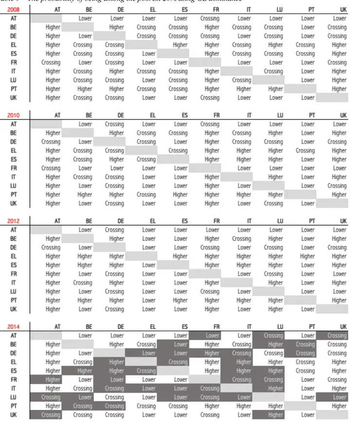
5. Dominance conditions of the probability of being poor
5.1 Extending dominance criteria to the probabilities of being non-poor
In the previous section, the analysis of poverty, which is typically developed on a distribution censored by the poverty line, has been extended to the overall distribution of probabilities of being non-poor by using ANOGI. Thus, our analysis differs from the standard way of dealing with inequality among poor, i.e. with inequality calculated among individuals that are below a poverty line, to favour a global view of the inequality of probabilities and thus a measure of the concentration of non-poor individuals.
In this section, using the same approach, a step further is done to investigate to what extent the ranking of countries according to the probability of being poor can be translated into wider social norms. To perform this task, we use the dominance criterion related to the generalised Lorenz dominance technique. To build this process, as before, we still use the complement of the estimated individual probability of being poor as an indicator of the position in the income distribution. In particular, individuals in each country can be ordered from the lowest to the highest probability of being non-poor, where the lowest probability of being non-poor will be 0 and the highest probability of being non-poor will be 1.
By ordering individuals according to this indicator, the outcome can be interpreted as an approximation of the usual ranking from the poorest to the richest individual. As a consequence, the dominance of the generalised Lorenz (GL) curve of the probabilities of individuals in country A over the generalised Lorenz curve of the probabilities of individuals in country B would mean that individuals in country A have less (probability of) poverty than individuals in country B for any fraction of the population. As in the previous section, the focus is on the whole distribution of probabilities – and thus on the total number of individuals – and not only on the distribution of probabilities of individuals below a given poverty line.
As it is well known, however, the GL dominance is not a synthetic measure, neither of inequality nor of poverty, which means that uncertain outcomes between countries may occur whenever the GL curves cross. In order to combine GL dominance with more general social prescriptions in the analysis of multidimensional poverty, recourse has been made to an extension of the well-established correspondence between classes of social welfare functions and dominance conditions.6
In our case, the GL dominance of a given distribution of the probabilities of being non-poor may be thought as more socially preferred, as the dominating distribution implies a higher probability of being non-poor for any fraction of the population. To this purpose, define a class of social norms L(¢) that satisfies L£(¢) > 0
and L££(¢) < 0. These two conditions only require that the social preference is increasing in the argument
(i.e., it increases when the probability of being non-poor increases) and concave, which means that a “transfer” of the probability of being non-poor from a higher to a lower probability would increase the social preference.7
Thus, GL dominance would allow general conclusions when comparing social preferences without the need to specify an exact functional form for L(¢).
6 See for all Lambert (1993) and Deaton (1997).
7 It is worth noting that this second condition is simply a restatement of the principle of transfers that holds when income is the argument