ISSN 2282-6483
Exchange Rates and Political
Uncertainty: The Brexit Case
Paolo Manasse
Graziano Moramarco
Giulio Trigilia
Exchange Rates and Political Uncertainty: The Brexit Case
∗Paolo Manasse1, Graziano Moramarco2, and Giulio Trigilia3 1,2University of Bologna, Department of Economics
3University of Rochester, Simon Business School
February 3, 2020
Abstract
This paper studies the impact of political risk on exchange rates. We focus on the Brexit Referendum as it provides a natural experiment where both ex-change rate expectations and a time-varying political risk factor can be measured directly. We build a simple portfolio model which predicts that an increase in the Leave probability triggers a depreciation of the British Pound, both on account of exchange rate expectations and of political risk. We estimate the model for multilateral and bilateral British Pound exchange rates. The results confirm the model’s main implications. When we extend the analysis to a portfolio model of multiple currencies, we find that the cross-currencies restrictions implied by the theory are not rejected by our system estimation. Moreover, the joint estimates of the multi-currency model in the presence of time-varying political risk premium are in many cases consistent with the Uncovered Interest Parity.
Key words: Brexit, Exchange Rates, Political Risk, Time-Varying Risk
Pre-mium, Uncovered Interest Parity
JEL classification: F31, F41, G11, G15.
1
Non-technical Summary
Politics has long been recognized as a major determinant of exchange rates. However, political risk is notoriously difficult to quantify. To overcome this hurdle, the recent literature has privileged breadth relative to depth, proposing indices of political uncer-tainty that aggregate over multiple sources of primary information, mainly from the press, and count the frequency by which a number of keywords, such as uncertainty, economy, deficit, tax policy, appear. This paper takes the opposite approach. We focus on a major recent political event—the Brexit Referendum in Great Britain—for which the response of currencies to political risk can be measured directly.
The Brexit Referendum has shaken the European and international political scene in 2016: for the first time a European Union (EU) member country, the UK, voted for leaving the Union. Indeed, with the unexpected victory of the “Leave” camp, the British Pound (BP) depreciated overnight by about 7% against the Euro and other main currencies. What makes the Brexit Referendum an interesting “natural experiment” for economists is that political risk can be measured with precision, because the event has been preceded by an exceptionally liquid betting market. Bookmakers, such as Betfair and PredictIt, provided online platforms on which individuals could bet on the likely outcome of the Referendum in real time. From the bookmakers’ odds, we can extract a daily series of the probability of Brexit and derive the “correct” measure of the political uncertainty associated with the Referendum result.
In the paper we ask a number of questions. The first is whether, and why, the evolution in the Leave probability is associated to movements in the price of currencies. To answer, we write down a simple model where risk-neutral investors form expectations about post-Referendum exchange rates, and where these expectations depend of their assessment of the Leave/Remain probabilities. In our benchmark estimates, we find that markets expected a depreciation of the BP against a basket of major currencies of approximately 20% in case of a Leave victory.
Our second question is whether there is evidence that currency markets price a po-litical risk premium. We extend the model by allowing investors to be risk-averse, and from the Leave probabilities we derive a formula for the premium associated to political risk. The estimates suggest that when the political risk factor increases the BP tends to depreciate with respect to all the currencies considered, since investors reallocate their investments to less risky assets.
Thus, as the probability of a Leave outcome increases, the BP depreciates due to two effects. The first operates via expectations: a more likely Leave outcome induces
investors to expect a future depreciation after the Referendum, so that the exchange rate weakens immediately. The second works trough the political risk premium: as the Leave probability gets closer to 50%, investing in BP becomes riskier and investors re-allocate their portfolios away from it.
Relating time-varying political risk and exchange rates is especially important in the context of the so-called “Uncovered Interest Parity (UIP) anomaly”, which refers to the puzzle that the spread between the domestic and the foreign-currency denominated assets tends to be either weakly or negatively correlated to the depreciation rate of the domestic currency, particularly at short maturities and for low-inflation countries, and so borrowing in the the low-rate currency and investing in the high-rate one—the so-called carry trade—allows investors to realize possibly unbounded profits. Thus, our third question is whether measuring political risk directly helps to reconcile the exchange rate behavior with the UIP. In this case, the empirical results are more nuanced, but go in the direction of reconciling the data with the theory.
Our last question is whether our portfolio framework can improve on the standard approach that considers exchange rates in isolation. Indeed, we find that the model’s restrictions are not rejected by the data and that they help reconciling the data with the UIP condition of arbitrage—especially for the EU and the US.
2
Introduction
Politics has long been recognized as a major determinant of the international price of currencies. However, political risk is notoriously difficult to quantify. To overcome this hurdle, recent work has privileged breadth relative to depth, proposing indices of politi-cal uncertainty that aggregate over multiple sources of primary information to generate widely applicable and relatively long time series (e.g., Baker, Bloom and Davis (2016)). In order to complement this literature and to dig into the mechanism by which politi-cal risk is priced, this paper takes the opposite approach. It focuses on a major recent political event—the Brexit Referendum in Great Britain—for which the response of cur-rencies to time-varying political risk can be measured directly. Our findings confirm that a time-varying political risk premium plays a crucial role in exchange rate determina-tion. Moreover, our theory-based methodology identifies the premium from economic fundamentals, and can be applied to the analysis of other political events.
The Brexit Referendum has shaken the European and international political scene in 2016: for the first time a European Union (EU) member country, the UK, voted for leaving the Union. The debate in the run-up to the Referendum focused mainly on
in-ternational issues, trade and immigration, which justifies our interest in the implications for exchange rates. With few exceptions, economists agreed that Brexit would have neg-ative consequences on the British economy (e.g., Sampson et al. (2016)),1 and expressed
concerns that the City of London would lose its role as the main market for Euro denom-inated assets (e.g., Reuters, 2016). Indeed, with the unexpected victory of the “Leave” camp, the British Pound (BP) depreciated overnight by about 7% against the Euro and other main currencies.
What makes the Brexit Referendum an interesting “natural experiment”, where po-litical risk can be measured with some precision, is that the event has been preceded by an exceptionally liquid betting market.2 Bookmakers, such as Betfair and PredictIt,
provided online platforms on which individuals could bet on the likely outcome of the Referendum in real time. From the bookmakers’ odds, we can extract a daily series of the (risk neutral) probability of Brexit. With the benefit of hindsight the level of political odds has been criticized, as it failed to predict the outcome,3 however we note that the
informativeness of the odds-implied probabilities should not be measured by the accu-racy of their levels, but rather by their ability to track changes through time, which is captured by our time-series regressions. Thus, our first question is whether, and why, the evolution in the odds-implied Leave probability before the Referendum is associated to movements in the price of the British Pound in terms of other currencies.
To answer, we start by writing down a simple model where risk-neutral investors form expectations about post-Referendum exchange rates. In the absence of arbitrage opportunities, the Uncovered Interest Parity (UIP) should hold, and the interest rate on a domestic currency-denominated asset should exceed the foreign one when the domestic currency is expected to depreciate. We extend the UIP condition allowing the expected depreciation to depend on the (time-varying) probability of Leave. We then take this model to the data, and find that, consistent with the post-Referendum outcomes, market participants expected the British Pound to depreciate against all major currencies upon a victory of the Leave campaign. In particular, our benchmark estimates suggest that the markets expected a depreciation of the BP against a basket of major currencies of approximately 20% in case of a Leave victory, regardless of whether the basket is weighted
1For example, a study byH.M. Treasury(2016) concluded that “taking as a central assumption that
the UK would seek a negotiated bilateral agreement, like Canada has, [...] our GDP would be 6.2% lower, families would be £4,300 worse off and our tax receipts would face an annual 36 billion black hole.”
2Mike Smithson, founder and editor of PoliticalBetting.com, defined Brexit as “the biggest political
betting event of all time, anywhere”. According to a Guardian column (June 24, 2016), “More than £40m was gambled in the biggest political betting event in British history.”
3See for example the Guardian (June 24, 2016) and the Independent (June 24, 2016). A notable
according to trade flows or international investment positions.4
While the odds-implied probability can be used to estimate the expected effect of Brexit on exchange rates (first moment), it also provides the basis to construct a time-varying political risk premium (second moment). Intuitively, the closer the odds-implied probability gets to one half, the closer the political risk faced by market participants gets to its peak, in a non-linear fashion. Thus, we can extend the model allowing the marginal investor in the currency market to be risk-averse, and derive a closed form solution for the time-varying risk premium, as a non-linear function of the Leave probability. Our
second question is whether there is evidence that currency markets price our
(model-based) measure of political risk premium.
The answer turns out to be clearly positive. Our political risk factor is positively and highly significantly associated to the BP price of a basket of other currencies and to bilateral exchange rates, with the exception of the BP-Japanese Yen, irrespective of the sample period considered and of the estimation method employed. Thus, as the probabil-ity of a Leave outcome increases, the BP depreciates due to two effects. The first operates via expectations: a more likely Leave outcome induces investors to expect a future de-preciation after the Referendum, so that the exchange rate weakens immediately.5 The
second works trough the political risk premium: as the Leave probability gets closer to 50%, investing in the BP becomes riskier and investors re-allocate their portfolios away from it.
The significance of our direct measure of the time-varying political risk factor comple-ments the recent work that stresses the importance of political uncertainty by studying aggregate indices (e.g.,Baker, Bloom and Davis(2016),Pastor and Veronesi(2012), Bro-gaard and Detzel (2015), Fernández-Villaverde, Guerrón-Quintana, Kuester and Rubio-Ramírez(2015) and Kelly, Pástor and Veronesi(2016)), in a setting where the definition of political risk is derived from the theory and can be measured from the bookmakers’ odds—a market price that conveys the ‘wisdom of the crowd’. Other related work on the price of political uncertainty has either focused on tax policies (Sialm(2009), Croce, Nguyen and Schmid (2012)), or on equity premia (Santa-Clara and Valkanov (2003),
Belo, Gala and Li (2013), Bittlingmayer (1998), Voth (2003), and Boutchkova, Doshi, Durnev and Molchanov (2012)).
4We focus on ten currencies, which are representative of the major British partners: Euro, US
Dollar, Japanese Yen, Swiss Franc, Canadian Dollar, Danish Krone, Swedish Krone, Norwegian Krone, Australian Dollar, New Zealand Dollar.
5This has also been documented in recent papers that focus on exchange rate predictability and
Brexit (e.g., Korus and Celebi (2018), Hanke, Poulsen and Weissensteiner (2018), Auld and Linton
(2019) andClark and Amen(2017)). None of these papers considers second moments—so their findings are unrelated to political uncertainty—or builds a model to interpret the result ‘structurally’.
In addition, our results relate to the vast literature on exchange rates. While recent work analyzed the pricing of macroeconomic uncertainty in currency markets (e.g.,Rossi and Sekhposyan(2015)), the role of political uncertainty has been largely overlooked. To our knowledge, the only exception isBachman (1992), who studies the impact of political news (elections) on the time-varying risk premium in foreign exchange markets. Before an election, there is uncertainty on whether the new government will implement a policy (a tax on domestic assets) which affects the domestic interest rate. This uncertainty is resolved after the elections. As a result, the parameters of an exchange rate equation should be unstable: those estimated in the sample before the elections should differ significantly from those in the post-election period. The author considers 13 election episodes in Canada, US, France and UK and finds evidence of parameter instability for about half of the episodes. Unlike Bachman (1992), we do not limit ourselves to testing for structural breaks, but we estimate the effects of time-varying political uncertainty on the exchange rate parameters.
Relating time-varying political risk and exchange rates is especially important in the context of the so-called “UIP anomaly”, which refers to the puzzle that while the arbitrage condition predicts that the domestic interest rate should rise to compensate an expected depreciation of the domestic currency, the spread between the domestic and the foreign-currency denominated assets is typically found to be either weakly or negatively correlated to the depreciation rate of the domestic currency, particularly at short maturities and for low-inflation countries (see Fama (1984), Hodrick (1987), Froot and Frankel (1989),
Burnside et al.(2006),Chinn and Quayyum(2012),Engel(2014) andIsmailov and Rossi
(2018)), and so borrowing in the the low-rate currency and investing in the high-rate one—the so-called carry trade—allows investors to realize possibly unbounded profits. The literature on exchange rates has tried to rationalize the puzzle either by positing a time-varying risk premium (e.g., Fama (1984), Verdelhan (2010), Lustig et al. (2011),
Bansal and Shaliastovich (2013),Farhi and Gabaix (2015)), or deviating from standard, rational preferences and beliefs (e.,g., Gourinchas and Tornell (2004), Burnside et al.
(2011),Ilut(2012)). In our paper, we do not make assumptions about the co-movement of exchange rate expectations and risk premia: we can measure it directly from bookmakers’ odds.
Thus, our third question is whether measuring political risk directly helps to recon-cile the exchange rate behavior with the UIP. Interestingly, the theoretical model implies that the “true” political risk-premium should co-move with the exchange rate exactly in the way required by Fama (1984) to explain the UIP puzzle.
basket of currencies and for the major trading partners of the UK (i.e., the US and the EU), we find that the spread between the domestic and the foreign-currency denominated assets tends to be positively correlated to the depreciation rate of the domestic currency, as the UIP requires. On the other, we often observe a higher coefficient than that predicted by the UIP, although the standard errors are too large to rule out that the coefficient is one (as required by the theory). Moreover, consistent with the previous literature, such coefficients seems to be quite unstable across samples and specifications, at least when we proceed estimating single equation models, currency by currency. Interestingly, the UIP performs much better when we take into account the cross-equation restrictions implied by the portfolio choice model and when we expand the sample period (see below).
It has also been extensively argued that testing the UIP might fail for econometric reasons. This may be either because a random walk model for the exchange rate typically outperforms structural models in terms of out-of-sample forecasts (see Meese and Rogoff
(1983a,b), Cheung, Chinn and Pascual (2005),Alquist and Chinn (2008)), or because of hard-to-predict rare catastrophic currency crashes (Brunnermeier, Nagel and Pedersen
(2008),Farhi and Gabaix(2015)), or because of biases in the standard errors (Baillie and Bollerslev (2000), Rossi (2006)), or because of small sample biases (Chinn and Meredith
(2005),Chinn and Quayyum(2012), andChen and Tsang(2013)), or due to time-varying volatility (e.g., Clarida et al. (2009), Menkhoff et al.(2012))
This leads to our fourth question, which is whether it is possible to improve on the standard approach of estimating single-equation exchange rate models by consider-ing a simultaneous, multi-currency settconsider-ing. In this respect, one interestconsider-ing property of our portfolio-choice approach is that it can easily be extended to a setting in which in-vestors choose between more than two currencies. The model helps us to identify one cross-equation restriction that should hold and improve the efficiency of the estimates. This restriction derives from two considerations: first, the coefficient of risk-aversion of the marginal investor should not vary systematically across currency-pairs; second, the optimal share of every currency in the portfolio should depend on the entire co-variance structure of exchange rates. Indeed, when estimating a dynamic Seemingly-Unrelated-Regressions (SUR) system, we find that our restriction is not rejected by the data, while the coefficients on both odds and odds-volatility remain similar and statistically signifi-cant for most countries. Moreover, relative to the currency-pair regression in isolation, the SUR estimates are more often significant and the UIP parameter of the interest rate differential is much closer to the theoretical value—especially for the EU and the US.
The paper unfolds as follows. Section 3 presents the theoretical model. First, we assume risk neutrality. Then, we introduce risk-aversion and consider a simple
mean-variance model of portfolio choice, which we extend in various directions. Section 4
presents the data. Section 5 discusses the empirical strategy, and presents the empirical results. The section also includes a number of robustness checks. Section 6 concludes.
3
The Model
In this section we lay out our reference model. We use the model to show that the parameters of the UIP condition must reflect the expectations of future exchange rates and are not “structural”. We start from a neutral setting, and then we introduce risk-aversion. This allows us to derive a time-varying political risk premium, as a function of observables. We then discuss two extensions. In the first one we add another source of political uncertainty in the pre-Referendum period, which reflects the possibility that the Referendum may or may not be called. This extension shows that equations parameters may exhibit jumps when important sources of uncertainty are resolved. The second extension considers a portfolio model with many currencies. This model implies that the parameters of different currencies are not independent and should satisfy a simple cross-equation restriction that we test on our data.
3.1
Risk-Neutrality, Two Currencies
This section develops the simplest framework where we can discuss exchange rate move-ments around the resolution of uncertainty of a major political event, such as the Brexit referendum. We denote by i and i* the domestic (UK) and foreign interest rates, which apply on assets denominated in the respective currencies.6 These assets are issued before,
and mature after, the date of the Referendum. The (natural logarithm of) the nominal exchange rates before and after the resolution of uncertainty on the Referendum outcome are denoted by e and e’, respectively, and both are expressed as units of the domestic currency (BP) for one unit of foreign currency. The UIP condition states that the dif-ference between the interest rates of a domestic and foreign-currency denominated asset must equal expected depreciation, and can be written as follows:
e = i∗− i + E(e′). (1)
6Throughout the analysis, we abstract from default risk. This seems a reasonable first-order
approx-imation, given that we are considering countries where default risk is considered to be fairly small—both in the sovereign CDS market and according to all major credit rating agencies.
where E denotes the expectation operator. For now, we assume that a Referendum will certainly take place. Given that there are only two possible outcomes of the vote,
V ={Leave (L), Remain (R)}, the exchange rate which is expected to prevail after the
vote is:
E(e′) = πE(e′|L) + (1 − π)E(e′|R), (2)
whereE(e′|V ) represents the expected exchange rate conditional on the vote V, and π is the ex-ante probability of a Leave vote. Substituting the previous definition into equation (1) yields:
e = i∗− i + π [(E(e′|L)) − (E(e′|R))] + E(e′|R). (3) Assume that the probability of a Leave outcome can be observed—for instance, from betting odds posted by risk-neutral wagerers. Then, a linear regression of the exchange rate on the foreign-domestic spread and on the odds probability yields:
e = θ(i∗− i) + α + βπ, (4)
where equation (3) implies the following:
α =E(e′|R), (5)
β =E(e′|L) − E(e′|R), (6)
θ = 1. (7)
The intercept parameter α in the regression is the market’s expectation of the future exchange rate conditional on a Remain victory, and the sum of the estimates of the inter-cept and slope coefficients α + β =E(e′|L) gives the expected exchange rate conditional on a Leave victory. A positive (negative) estimate of the coefficient β implies that the exchange rate is expected to exhibit a jump depreciation (appreciation) after the Ref-erendum if the Leave outcome prevails. The probability of Leave π takes the value one after the Referendum date, as this source of political uncertainty gets resolved.
3.2
Risk-Aversion, Two Currencies
In this section we assume that investors are risk averse and derive a precise measure of the political risk premium. Consider a representative foreign (i.e., non-UK) investor who chooses between investing in its own currency denominated asset, which is safe, or in a BP denominated asset, which is risky because of exchange rate fluctuations. The portfolio choice occurs before the resolution of uncertainty on the Brexit Referendum, as
the assets mature after the vote. Let the portfolio share that is invested in the UK be
ω. For simplicity, we consider standard mean-variance preferences, so that the investor
chooses ω in order to maximize:
U (ω) = (1− ω)i∗+ ω [i− (E(e′)− e)] − r 2ω
2σ2, (8)
where r ≥ 0 is the coefficient of absolute risk-aversion and σ2 is the portfolio variance.
In equation (8), the first term on the right side represents the return on the risk-free non-UK (safe) investment, i∗, while the second term represent the expected return on the UK (risky) investment, given by the sum of the interest rate i and the expected appreciation of the BP. Each term is weighted by its respective portfolio share. The last term in the utility function is the product of the risk-aversion parameter r
2 multiplied by
the (squared) share of UK assets times the risk on the portfolio return, σ2.7 The portfolio
variance reads:
σ2 = πE[e′|L]2+ (1− π)E[e′|R]2−(πE[e′|L] + (1 − π)E[e′|R])2
= π(1− π)[E[e′|L] − E[e′|R]]2
= π(1− π)β2 (9)
Equation (9) shows that the portfolio variance coincides with the volatility of the exchange rate. This volatility increases with the difference between the expected exchange rates conditional on the two possible outcomes, β (see (6)), and reaches a maximum when the Leave/Remain probabilities are the same, or π = 1
2. From the first-order condition, the
optimal portfolio share of UK-denominated investments reads:
ω = i− (E[e
′]− e) − i∗
rσ2 . (10)
Intuitively, the share in BP denominated assets is an increasing function of the difference between the UK and the foreign expected yields. With risk-averse investors–i.e., r > 0— the share of BP denominated assets is decreasing in the portfolio volatility σ2 and in the
degree of risk-aversion. We can solve for the exchange rate e by assuming that the asset market clears, so that the demand for foreign assets (ω) equals supply (s), that we take as exogenous.8 Substituting ω = s in (10) and solving for the exchange rate we obtain a
7The term ω2follows from the property that, for a random variable X: Var[ωX] = ω2Var[X]. 8This assumption is relatively innocuous in the short-run, when the supply of currencies hardly
modified UIP condition:
e = θ(i∗− i) + α + βπ + γπ(1 − π), (11)
where:
α =E[e′|R] > 0, β = E[e′|L] − E[e′|R], γ = rβ2s ≥ 0, θ = 1.
This expression generalizes equation (4) for the case of risk aversion, with the addition of a time-varying risk premium given by rσ2s = rπ(1− π)β2s. This premium is increasing
in the equilibrium portfolio share of BP (that is, s) in the coefficient of absolute risk-aversion (r), and in the volatility of the portfolio return (σ2). The risk-premium will be
time-varying as long as the probability of Leave, π, changes over time. Note that a marginal increase in the Leave probability (from below 1
2) now has two
separate effects on the current exchange rate. On the one hand, it implies a rise in the future expected exchange rate—provided that the investors forecast a weaker BP in case of Brexit, i.e. β > 0. On the other hand, a larger Leave probability raises the political uncertainty, leading risk-averse investors to reduce their portfolio share of BP and further depreciating the exchange rate. Thus, a larger Leave probability π raises the current exchange rate e by more than it raises the future expected exchange rate E(e′), and this overshooting implies an expected appreciation of the currency. As a result, a change in the Leave probability induces a negative correlation between the risk premium and the expected depreciation rate, as required byFama (1984) to solve the UIP puzzle.
3.3
Referendum Uncertainty, Two Currencies
In our framework, the parameters of the exchange rate equation α, β and γ depend on the “deeper” parameters which reflect agents’ information and preferences, and which may be subject to change when crucial Brexit-related news arrive. We dig further into this issue by considering an alternative reason for parameter instability: the resolution of uncertainty on the Referendum itself. To this end, we extend the model by taking a step backward in time when, following the UK negotiations with the EU, investors were uncertain on whether a referendum on Britain’s membership of the EU would ever be called. This extension tries to rationalize what happened when the British Parliament promulgated the so called “Referendum Act” in mid December 2015, which established the constitutionality of a Referendum on the membership of Great Britain in the EU and made sure that a vote will be called. As we will discuss later on, three things happened in the following weeks: currency markets reacted with a sharp depreciation
of the BP; the different Bookmakers odds on the outcome of the vote, which until then show little correlation among themselves, started to converge and comove; and finally, their correlation with exchange rate increased sharply. Let q denote the probability that a referendum will take place, so that with probability 1− q the Referendum will not take place, in which case the exchange rate is expected to beE[e′|∅]. In this case, the expected exchange rate is
E(e′) = (1− q)E[e′|∅] + q JπE(e′|L) + (1 − π)E(e′|R)K
which is a linear combination of the expected exchange rate conditional on no Referen-dum, the first term, and the expected exchange rated conditional on the Referendum taking place. It is easy to show that, in the case of risk neutral investors, the exchange rate equation is modified as follows:
e = θ(i∗− i) + α + qδ + qβπ,
where α, β, θ are defined as before and δ =E[e′|R] − E(e′|∅). In particular, if the market anticipates that the exchange rate that will prevail after a Remain vote will be the same as the one that would have prevailed had the Referendum not occurred, δ = 0, the equation simplifies to
e = θ(i∗ − i) + α + qβπ. (12)
Comparing (12) with equation (4) we can see that the coefficient of the Leave probability,
π, should make a discrete jump from qβ to β at the moment when the Brexit Referendum
is announced. Intuitively, at this moment the effect of the odds on the expected exchange rate will increase. A similar intuition holds for the portfolio model with risk aversion. In this case, it is easy to show that introducing uncertainty on the actual occurrence of the Referendum modifies the exchange rate equation as follows:
e = θ(i∗− i) + α + qδ + qβπ + γqπ(1 − π), (13)
where the parameters α, β, γ are the same as in (12). This equation shows that also the coefficient of the risk-premium π(1−π) should exhibit a discrete upward jump at the time of the Referendum announcement. The portfolio variance now reads σ2 = qπ(1− π)β2.
3.4
Risk Aversion, Many Currencies
Our portfolio model immediately generalizes to the case of many currencies, where the (non-UK) investor can chose between N + 1 assets, one denominated in his own currency and N denominated in foreign currencies, with yields denoted by i, j = 1, . . . , N . The portfolio weights are denoted by ωj. For simplicity, we consider the case in which the
Referendum is known to take place for sure. Let ej denote the price of currency j in terms
of the investor’s currency. Investing in a currency j entails a currency risk due to the Referendum. We need to replace the previous objective function (8) with the following expression: U = (1−∑ j ωj)i∗+ ∑ j
ωj[ij−(πE[e′j|L]+(1−π)E[e′j|R]−ej)]− r 2 ∑ j ωj2σj2+ 2∑ i ∑ j>i ωiωjσij ,
where the portfolio variance now depends on the weighted sum of all bilateral variances and covariances σij. Using the fact that:
E(e′ie′j) = π[E[e′i|L]E[e′j|L]]+ (1− π)[E[e′i|R]E[e′j|R]],
we can write the covariance between two currencies i and j as follows:
σij = E(e′ie′j)− E(e′i)E(e′j) = π(1− π)
[
(E[e′i|L] − E[e′i|R]) (E[e′j|L] − E[e′j|R])] = π(1− π)βiβj.
This expression shows that the covariance between any pair of currencies is equal to the product of the expected “jumps” β of the two currencies, multiplied by the uncertainty over the Referendum outcome π(1− π). This extends equation (9) to the case of many currencies. Proceeding as before, we can calculate the optimal portfolio shares, ωj , and
derive the equilibrium price equations, j = 1, . . . , N satisfying ωj = sj. We obtain:
ej = i∗− ij +E[e′j|R] + π(E[e′j|L] − E[e′j|R]) + r
∑
j
∑
k>j
sjskσjk
which we can rewrite in compact form as
where
αj =E[e′j|R], βj =E[e′j|L] − E[e′j|R], ˜γ = r
∑
j
∑
k>j
sjskβjβk, θ = 1, for j = 1, ..., N
Expression (14) represents a system of N non-linear equations. This system is charac-terized by a cross-equation restriction on the parameters. The restriction comes from the fact that, unlike the intercept αj and the slope βj which are country-specific, the
coeffi-cient of the volatility term, ˜γ, depends on the expected “jumps” of all the exchange rates
in the portfolio and on the risk-aversion parameter, and should therefore be identical across currencies.
In this model, the coefficient of the political risk premium term, ˜γ, can in principle
be negative, so that the BP would “appreciate” when political risk increases. This would apply if the British Pound, in case of Leave, were expected to appreciate relative to some currency j and to depreciate relative to some other currency k, βj < 0, βk > 0. In these
(unlikely) circumstances, investing in BP may entail a diversification benefit which would reduce exposure to political risk. This extension suggests that imposing the restriction that the volatility coefficient should be the same across currencies and estimating a system of equations could improve the efficiency of the estimates.
4
The Data
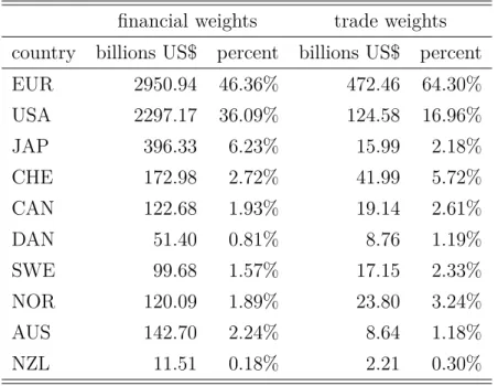
For the empirical analysis we collected daily data from May 27, 2015, to June 23, 2017 on exchange rates, interest rates, bookmakers odds, as well as other measures of political and economic uncertainty suggested by previous research. We study the behavior of the British Pound (BP) vis-à-vis the currencies of a number of major trading partners among advanced economies: the Euro (EUR), the US Dollar (USA), the Japanese Yen (JAP), the Swiss Franc (CHE), the Canadian Dollar (CAN), the Danish Krone (DAN), the Swedish Krone (SWE), the Norwegian Krone (NOR), the Australian Dollar (AUS) and the New Zealand Dollar (NZL). To this aim, we consider two specifications of a multilateral nominal exchange rate of the BP against a basket of these ten currencies, as well as each bilateral exchange rate.
Our first multilateral exchange rate (and the corresponding interest rate differential) is constructed as a weighted average of the country-specific exchange rates (interest rates), using trade weights—based on international trade flows between the UK and the other countries. More specifically, each trade weight is calculated as the ratio of the bilateral trade (the sum of exports and imports) to the total value of UK trade with the ten
countries, measured in 2015. We also construct an alternative measure of multilateral exchange rate based on financial weights. Specifically, for a generic country i, the financial weight is given by the ratio of the financial position (the sum of assets and liabilities) of the UK towards country i, relative to the total financial position of the UK against all the other ten countries, measured as of December 2015.
Table 1 reports the two sets of weights in column 2 and 4, and the value of bilateral trade and of the bilateral financial position in 2015 in column 1 and 3, respectively. In both exchange rates the Euro and the USD play a dominant role. The trade-weights reflect the predominant share of the EU in UK trade (64.3 percent) with a relatively minor role for the USD (17 percent) and a non-negligible role for the Swiss Franc (6 percent), while financial weights are relatively more balanced, and assign to the Euro and the USD respectively 46 and 36 percent, and about 6 percent to Japan. The data source for the exchange rates and interest rates is Datastream. As in Ismailov and Rossi
(2018), the interest rates considered here are 3-month euro LIBOR rates. The source for international financial positions is the IMF Coordinated Portfolio Investment Survey (CPIS). International trade data are from the IMF Direction of Trade Statistics (DOTS). Our Leave probability measure is constructed using real time data provided by two betting companies: Betfair and PredictIt. For either provider, we take the daily average probability of Leave derived from the corresponding odds. The probability variable π is the average of the two series. We chose to use these data as we consider that these prediction markets reflect the ‘wisdom of the crowd’. In particular, unlike survey data, they are immune from misreporting as investors “put their money where their mouth is”. In the words ofArrow et al.(2008), “because information is often widely dispersed among
economic actors, it is highly desirable to find a mechanism to collect and aggregate that information. Free markets usually manage this process well because almost anyone can participate, and the potential for profit (and loss) creates strong incentives to search for better information”. Prediction markets are used to manage risks—such as flu outbreaks
and environmental disasters—by public entities (e.g., U.S. Department of Defense) as well as firms (e.g., General Electric, Google, France Telecom, Hewlett-Packard, IBM, Intel, Microsoft, Siemens, Yahoo).
Betfair is a British online gambling company headquartered in Hammersmith (West London) and Clonskeagh (Dublin). It claims to have over 4 million customers (1.1 million active customers) and a turnover in excess of £50 million a week. As of April 2013, the company employed 1,800 people. In its betting website, Betfair listed two Brexit-related contracts. The first paid out £1 in the event of a Leave victory, the other paid £1 in the event of Remain. Betfair supplied us with the odds implicit in the contract prices,
which are observed from 5/27/2015 to 6/24/2016 at different time-intervals (often of 1 second), each week day for a total of 143,290 observations. This data source was used in recent papers, e.g., Auld and Linton (2019). We complement this with a second source for betting odds, the New Zealand-based company PredictIt, which launched a market on the Brexit vote on November 3, 2014 and caters mainly US-based investors.9
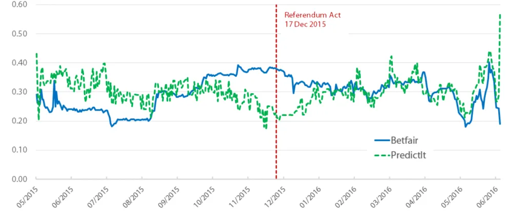
Figure 1 compares the two Leave probability series derived from the Betfair odds (solid blue line) and the PredictIt ones (dashed green line). The figure reveals that the Leave probability measures were quite noisy in 2015: until December 2015, the two series exhibit a negative correlation (-0.35) and the standard deviation of their difference is 9.30%. However, starting in January 2016 the odds appear to behave similarly: for the period January 1 - June 22 the standard deviation falls to 4.23% and the correlation coefficient rises to 0.51.
Among a series of relevant political events which marked the run-up to the Referendum and the progress of UK-EU negotiations, two dates were pivotal, at least according to the briefing paper by the UK House of Commons Library on Brexit (Walker(2018)): the first is December 17, 2015—when the EU Referendum Act was promulgated—and the second is February 22, 2016—when Prime Minister David Cameron announced that the Referendum would take place on June 23, 2016. The Referendum Act was the act of the Parliament that made legal provision for a consultative referendum to be held in the United Kingdom and Gibraltar, on whether the UK should remain a member state of the European Union or leave it. Following the Royal Assent to the Act, although the Prime Minister did not indicate a precise date for the vote, the British media considered June 2016 as the most likely period well before David Cameron’s official announcement.10
A dashed vertical line in Figures 1-2 identifies the date (December 17, 2015) on which the European Union Referendum Act received Royal Assent and was therefore promulgated.
9Investors in PredictIt buy assets whose price represents the probability of a certain outcome (e.g. a
Leave victory) and can hold the asset until maturity (the Referendum day) or trade it before maturity, at the ongoing price. In order to comply with U.S. regulators, PredictIt caps the size of trading positions (seeWolfers and Zitzewitz(2018)). We do not have information on individual traders, however Predic-tIt described to us its investors as follows: “they are affluent (100-200k annual income), well-educated
millennials, aged 22-35, living in metropolitan areas like NYC, DC, Philadelphia, Dallas, Chicago, and San Francisco. Most traders work in finance, law, politics, and technical fields, such as mathematics, statistics, and economics. They are politically diverse with Democrats, Republicans, libertarians, “un-affiliated” or “no party” affiliates all using the site. There are about 30-35k active traders on PredictIt (defined as someone with money in their account) at any given time, with people entering and exiting markets regularly. Nearly 180,000 people have opened an account at the time of writing.”
10See, e.g.,the Telegraph (Dec. 18, 2015),the Independent (Dec. 18, 2015)and the Guardian (Jan.
Figure 2 plots the average of the two Leave probability series (solid blue line, left scale) along with the effective exchange rate of the BP against the basket of ten cur-rencies (dashed yellow line, right scale), using financial weights. Interestingly, around the approval of the EU Referendum Act, the exchange rate exhibits an upward move-ment (a depreciation of the BP of approximately 10%), while the correlation between the two variables increases—it is 0.18 from May 27 to December 17, 2015, it rises to 0.57 in the subsequent period. The graphical evidence and the descriptive statistics suggest that from late 2015 the odds associated to the bets on the Referendum result may have played a stronger role in explaining the BP exchange rate movements, consistently with the implication of our model.
The additional measures of political and economic uncertainty that we collected will be introduced in the robustness section, as they are not employed in our baseline estimation. Figure3plots all (log) exchange rates considered in this paper, from 27 May 2015 to 23 June 2017. The financially-weighted basket and the trade-weighted basket are denoted by ROWF and ROWT, respectively (where “ROW” stands for “rest of the world”). The
figure shows that, qualitatively, the BP exhibited similar patterns relative to the curren-cies considered in the paper, with a large depreciation occurring around the Referendum Act of mid December 2015.
5
Empirical Analysis
In this section we estimate a version of the Uncovered Interest Parity relationship implied by the theoretical model, which emphasizes the role of market expectations and of the political risk premium that are embodied in the odds of Leave. For this purpose we focus on the long-run (cointegration) relationship between the exchange rates and its determinants. We do so for different currencies, sample periods and by employing different statistical estimators. Thus we leave aside short-run dynamics issues. Estimates of an Error Correction Model, available upon request, confirm the results presented here and show that the exchange rates converge over time to this long-run relationship.
5.1
Setup
Based on equation (11), the impact effects of the Leave probability and of the political risk premium on the exchange rate of the BP may change as a result of a shift in mar-ket expectations on the future exchange rate. Equation (13) introduces the additional possibility that these effects may change as the result of a shift in q, the probability of
the Referendum being held.11 The approval of the Referendum Act, by removing the
un-certainty over the Referendum, in our interpretation affects the parameter q. Although we do not directly observe this probability, since there were no betting markets on the possibility of a vote, we will assume that this parameter takes the value of one after the date of promulgation of the Act, τ .
Therefore, our approach consists in estimating equation (13) under the assumption that a discrete upward shift in q occurs at the date of the promulgation of the EU Referendum Act: qt= q0 if t ≤ τ 1 if t > τ with q0 < 1.
We first estimate equation (13) for the effective exchange rate of the BP vis-à-vis our two baskets of ten currencies (either with financial-weighting or with trade-weighting of the countries). Next, we proceed to the analysis of country-by-country equations for bilat-eral exchange rates. Finally, we consider the joint estimation of a multi-currency portfolio model, allowing for cross-currency shock correlation and cross-equation constraints. Our benchmark sample spans the period from 27 May 2015, which is the first day when the odds on the Referendum outcome are available, to 30 June 2016. We include a few days after the vote for identification purposes. We also estimate the equations on a longer sample ending in June 2017.
Because the Leave probability never exceeds 50% before the vote, our volatility mea-sure π(1− π) is a monotonic transformation of π and the correlation between the two variables is close to 1. Collinearity would make their individual coefficients not identified and lead to inaccurate estimates.12 On 24 June 2016, the day after the vote, π jumps
to 1 and π(1 − π) drops to 0, as the Leave camp prevails and uncertainty about the outcome of the Referendum is resolved. Accordingly, the inclusion of post-referendum observations helps us to identify β and γ by exploiting the opposite movements of π and
π(1− π) following the vote. In the robustness section, we will make sure that our
esti-11Alternatively, q may be interpreted as a measure of the attention paid by investors to the odds on
the Referendum, thus capturing such factors as the expectations on the timing of the Referendum.
12This issue is reminiscent of the long-standing “peso problem” in the international macro literature,
which refers to the measurement of exchange rate expectations (or, more generally, asset-price expec-tations) and risk premia in samples that do not include large infrequent events, such as devaluations (Engel(2014)). Similarly, if we limited the sample to the pre-Referendum period, we may not be able to disentangle the contributions of the expected exchange rate and of the risk premium to the exchange rate movements.
mated coefficients on π and π(1− π) do not not simply capture a pre-post Referendum time effect.
Before presenting the results, we test our variables for the presence of unit roots and cointegration.
5.2 Unit Roots and Cointegration
Table 2 shows the results of the augmented Dickey-Fuller (ADF) test for unit roots in e and i∗−i, both over our benchmark sample 5/27/2015-6/30/2016 (“short sample”), which covers a few days after the Referendum, and over a sample period 5/27/2015-6/23/2017 (“long sample”), in which about half of the observations lie before and half after the Referendum. We choose to test the (non-)stationarity of the interest spreads, rather than the individual interest rates, because we will impose the theoretical restriction that it is the difference of yields that enters the UIP condition. All exchange rates appear to be non-stationary at any conventional level of significance on both samples. For the interest rate differentials, the results are more heterogeneous across countries and samples. Both the average differential based on financial weights and the one based on trade weights are non-stationary over the long sample, while the test rejects the presence of a unit root for both over the short sample. The interest rate differential appears non-stationary on both samples for the Euro area, USA, Japan, Canada and Denmark at the 5% level of significance, while for the remaining countries the null cannot be rejected in one of the two samples.
Table 3shows the results of the ADF test for π. In this case, the results are reported for the pre-Referendum sample 5/27/2015-6/22/2016 (for any sample ending after the Referendum, the test fails to reject the null due to the jump of π following the vote). As suggested by Figure 2, the Leave probability is stationary before the Referendum. In addition, the table presents the results for qπ, using two values for q0 –the perceived
probability of the Referendum prior to the Referendum Act. We will discuss the issue of how to estimate this parameter in the next paragraphs. For the moment we assume that this prior can take two values, q0 ∈ {0.25, 0.5}, which turn out to be plausible according
to our estimates. In either case, the unit root hypothesis is not rejected for the interaction variable qπ. This is the result of the upward shift in q at the time of the promulgation of the Referendum Act.
Given our specification (13), we test for cointegration between e, i∗ − i, qπ and
qπ(1− π), using the Phillips-Ouliaris residual-based test for single equations. The null
q0 ∈ {0.25, 0.5}. The results for q0 = 0.25 are reported in Table 4. At the 10% level
of significance, the test unambiguously indicates cointegration in the case of the effec-tive exchange rate, both financially-weighted and trade-weighted. Looking at individual currencies, the evidence is mixed, but on balance it appears mildly consistent with our hypothesis of cointegration: for all currencies except the Norwegian krone and the Aus-tralian dollar, the null of no cointegration is rejected at the 10% level of significance in at least one of the two samples. When we perform the cointegration test assuming q0 = 0.5
(Table 5), it signals cointegration at the 10% level in most cases. The interaction of π and π(1− π) with q is critical for establishing a cointegration relationship: when the test is conducted using the variables π and π(1− π), cointegration is generally ruled out.
5.3 Estimation Results.
This section presents our main results. We begin by considering ordinary least squares (OLS). The OLS estimator is known to be “superconsistent” (i.e., it converges in proba-bility to the true parameter value at a speed of T , the sample size, rather than the usual
T1/2) when the variables are non stationary but cointegrated. However, the estimator has an asymptotically biased and non-normal distribution, and does not allow for stan-dard inference. Moreover, as noted by Banerjee et al. (1986), the OLS estimator can suffer from substantial finite sample bias, and cointegration relationships should be in general estimated through dynamic regressions rather than static regressions. Maddala and Kim (1998) review the finite sample evidence on estimators of cointegrating vectors provided in Monte Carlo studies and advice against estimating long-run parameters by static regressions.
For these reasons, we turn to the dynamic ordinary least squares (DOLS) estimator, proposed by Saikkonen (1991) and Stock and Watson (1993). We also show results ob-tained using the fully-modified OLS (FMOLS) proposed by Phillips and Hansen (1990). Unlike the OLS, these estimators are asymptotically efficient in the presence of cointe-gration and allow for inference on the coefficients of I(1) variables, as their test statistics have conventional asymptotic distributions. As highlighted byRossi(2013), cointegration vectors are typically estimated by DOLS in the literature on exchange rates.
The DOLS estimator applies a parametric correction to the OLS in order to account for the correlation between residuals and regressors. In practice, the estimator is ob-tained by augmenting the cointegration regression with lags and leads of first-differenced
regressors. More specifically, in our case the benchmark DOLS regression is given by: et= θ(i∗t − it) + α + βqtπt+ γqtπt(1− πt) + δqt+ h ∑ j=−l ϕ′j∆Xt+j+ εt (15)
where Xt+j ≡ [i∗t+j − it+j, qt+jπt+j, qt+jπt+j(1− πt+j)]′, for every j, ∆Xt+j = Xt+j −
Xt+j−1, ϕj is a 3× 1 vector of parameters, for every j, and εt is an error term.
We employ an automatic lag/lead selection based on the Bayesian information cri-terion. This indicates that only contemporaneous differences should be included in the regression, regardless of the value of q0. Nevertheless, we also include lags and leads
of order 1 (i.e. l = h = 1) in order to capture more adequately the dynamics of our dependent variable.
We also employ the FMOLS estimator, which applies a different correction to OLS. It controls for the correlation between the error term of the cointegrating regression and the innovations of the regressors using a non-parametric consistent estimate of the long-run covariance matrix.
Table6reports the estimates obtained in the shorter sample by OLS, DOLS, FMOLS for the financially-weighted effective exchange rate (ROWF) and the trade-weighted
ef-fective exchange rate (ROWT). In order to obtain estimates for q
0, we actually make use
of non-linear least squares.13
The table shows that the estimated coefficients of the Leave probability and the political risk premium, β and γ respectively, are both positive and highly significant across all estimation methods. In our interpretation, β measures the percent BP depreciation rate that the market prices in the Leave scenario, relative to the Remain scenario. The value of the BP conditional on Leave is estimated to be around 19%-22% lower than the value under the Remain scenario. Importantly, a positive coefficient for our measure of
13More specifically, we use the Gauss-Newton algorithm for the numerical minimization of the sum
of squared residuals. In the case of DOLS and OLS, we optimize over all parameters simultaneously. To make sure that we detect a global minimum, we repeat the optimization 1000 times, each time using random draws from uniform(-10,+10) distributions as the starting values of the parameters. In the case of FMOLS, estimating q0 and the other parameters simultaneously is unfeasible. Therefore, we follow
a 2-step procedure in each iteration of the optimization algorithm: we first set a value for q0, then we
estimate the remaining parameters using conventional (linear) FMOLS, conditional on q0. Thus, in this
case we optimize numerically over q0only. For DOLS and OLS, the standard errors of the parameters are
obtained using the Newey-West heteroskedasticity and autocorrelation (HAC) estimator. For FMOLS, the standard error of q0is calculated asbσlr(h/2)−1/2, wherebσlr is the long-run standard error of FMOLS
residuals and h is the second derivative of the objective function (the sum of squared residuals) with respect to q0. This approach follows conventional methods for calculating standard errors of non-linear
regressions from the Hessian matrix (Amemiya(1983)). For the other parameters, we calculate ordinary FMOLS standard errors, conditional on q0.
time-varying political risk premium, π(1− π), means that higher Brexit uncertainty is associated with a BP depreciation. More generally, our approach allows to disentangle the two channels (first and second moments) by which the odds affect the exchange rate. For instance, let us consider what the model predicts should happen to the BP after the Leave victory, using the estimates in the first column of Table6. Given the average value of π (0.3) and π(1−π) (0.21) before the Referendum, the model predict a BP depreciation of about 7 percent. This is the net effect of: (i) the surprise of the Referendum outcome, which accounts for a depreciation of 14.8% = (1− 0.3) · 0.2112; (ii) an appreciation effect due to the resolution of uncertainty: −8% = (0 − 0.21) · 0.3834. The net result is a depreciation rate of ≃6.8%.
Table 6 presents another very interesting result. Unlike a large body of literature that found negative coefficients on interest rate differentials in the UIP relationship, we obtain the a-priori correct positive sign in our estimates for θ, although with high standard errors. The point estimates are generally higher than one, but they are not significantly different from 0. The model for the basket of currencies does not violate the UIP, as the hypothesis θ = 1 cannot be rejected.
The DOLS estimates of q0 are 0.26 and 0.2 for ROWF and ROWT, respectively, with
large confidence intervals (at the 90%, the parameter lies between 0 and 0.6 approxi-mately). The estimates are somewhat lower for FMOLS and OLS.14 Thus, as expected,
the effects of the odds variables are much higher after the Referendum Act, which con-firms the intuition that only when market participants perceive that the Referendum will take place for sure, they start placing more weight on the evolution of the odds.15 Also,
the coefficient δ on the variable q (non-interacted) is not significant, except for FMOLS estimates for ROWT. This is consistent with the assumption that market participants
expected the same value for the exchange rate in the case of No Referendum and in the case of a Remain victory. If the non-interacted q variable is omitted from the regression, the estimates of q0 become larger and significant, but still remain below 0.5 (the DOLS
point estimates are around 0.44 for ROWF and 0.43 for ROWT).
In our interpretation, the term α + δq gives the expected (log) exchange rate con-ditional on a Remain vote. This implies that the multilateral (financially-weighted)
14Note that the standard errors of q
0 in Table6are obtained without imposing that q0 lies between
0 and 1. So, for instance, the 90% confidence interval of the DOLS estimate for ROWF has a lower
bound of -0.08 and an upper bound of 0.59 approximately. To impose 0 < q0 < 1, we can use the logit
transformation of q0, denoted by λq, i.e. we can replace q0with exp(λq)/(1 + exp(λq)) in the regression.
In this case, while the point estimate of q0 remains the same, the lower and upper bounds of the 90%
interval are 0.06 and 0.66, respectively.
15The Wald test for the hypothesis q
0π = 0 has a p-value of 14%, for q0π(1− π) = 0 the p-value is
BP exchange rate after the Referendum Act (q = 1) should be approximately equal to exp(α + δq) = exp(−0.5046 − 0.0515) = 0.57, which is close but below the average rate prevailing before the Referendum Act (see Figure2).
Tables 8-10report the DOLS estimates for each individual currency. Here we impose the a priori restriction that q0 is the same for all countries, and equal to 0.25.16
The coefficient on the Leave probability qπ is positive and significant at the 1% level for all currencies, with point estimates ranging from 0.17 to 0.30. The coefficient on
qπ(1− π) is also positive for all countries and significant at the 1% for all countries
except Japan (for which it is not significant), Norway (for which it is significant at the 10%) and New Zealand (for which it is significant at the 5%). The estimates for the interest rate spread coefficient θ exhibit large cross-sectional variability. However, for all countries except Japan and Sweden, the point estimate is positive. Due to the large standard errors, the coefficient is not significantly different from 1 in the equations for the Euro, the Swiss franc, the Swedish krone, the Australian dollar and the New Zealand dollar. For the other currencies, the UIP is violated.
As shown in Tables9to11, our main results remain valid when we extend the sample by including one year of post-Referendum observations. In all equations, the estimates of the Leave probability coefficient, β, are larger and those of the risk-premium coefficient,
γ, are lower than over the short sample, but in general the estimates are very similar.
Moreover, the estimates of the interest spread coefficient, θ, are now closer to the theo-retical value of one both for the basket of currencies and for individual currencies, with the exceptions of the Swiss franc and the Australian dollar. Notably, the UIP is now not violated by the US dollar either.
5.4
Robustness Checks for Single Equation Estimation
5.4.1 Robustness to a Pre-Post Referendum Time Effect
As a first check, we show that our Leave probability and risk-premium variables do not simply capture a pre-post Referendum time effect.
We do this in two ways. First, we limit the sample to the pre-Referendum period and estimate the model under risk neutrality (i.e., excluding the volatility variable) in order to circumvent collinearity, and show that the Leave probability is indeed significant. Second, we include in the model with risk neutrality a pre-post Referendum time dummy,
dvote, and estimate the equation using both pre- and post-Referendum observations.
16Accordingly, the standard errors in Tables 8-10 are conditional on q
0 being known, whereas the
The results of the two regressions are reported in Table12, in column 1 and 2 respec-tively.
In both equations, the estimate for the Leave probability is positive, significantly different from zero and larger than the benchmark estimate of β in Table 6. This result is consistent with the fact that the risk-premium variable, which typically entered with a positive sign, is now omitted in both equations.
The second equation, which exploits post-Referendum observations, shows that the time dummy dvote enters with a negative and significant coefficient, which means an
appreciation of the BP in the aftermath after the vote. This is consistent with our model, which implies that the resolution of uncertainty and the consequent drop of the risk premium, now captured by the time dummy, should lead to an appreciation of the BP.
5.4.2 Unrestricted Break Model
In our benchmark equation we have posited that a structural break occurs around the promulgation of the EU Referendum Act. This section shows that this assumption is supported by the data and that is largely inconsequential for the estimation results.
We estimate the basic model (11) by DOLS and perform the Quandt-Andrews test for parameter instability at one unknown break date. We thus allow the data to determine if and when the coefficients of π and π(1− π), i.e. β and γ, exhibit structural breaks. We use a “pre”/“post” suffix to denote the parameter estimates for the pre/post - break period.
Table 13 shows the results for the multilateral exchange rates ROWF and ROWT.
For both the trade- and the financially-weighted rates we strongly reject the hypothesis that the coefficients do not change during the sample period. In both equations, we estimate a break occurring on Jan. 7, 2016—only a few weeks after our prior of a break, Dec. 17, 2015. Importantly, in the post-break sample the estimated coefficients of the Leave probability and the risk-premium, βpost and γpost, are strongly significant and not
statistically different from our benchmark estimates for both exchange rates (see Table
6), while the coefficients are not significantly different from zero in the pre-break period. Note, however, that this can be due to the fact that the covariates π and π(1− π) in the pre-break sub-sample are highly collinear, and this may impair inference about their individual coefficients.
An F -test rejects the null hypothesis that the Leave probability and the risk premium are jointly non significant before the break in the case of ROWF, while the p-value is
Overall, these results confirm that our assumption of a structural break occurring at the time of the Referendum Act is consistent with the data, and that the assumption does not drive the estimates of the other coefficients.
5.4.3 Alternative Uncertainty Measures
The present and final section on robustness compares our model-based measure of political risk premium with four standard measures of financial and economic uncertainty. In particular, we show here that our measure based on the bookmakers’ Leave probability is robust to their inclusion.
The first measure that we consider is the Economic Policy Uncertainty (EPU) index for the UK developed by Baker et al. (2016). The index is constructed by counting newspaper articles that contain at least one term from each of three sets of keywords: (i) economic or economy; (ii) uncertain or uncertainty; (iii) policy-related words: spending, deficit, regulation, budget, tax, policy, and Bank of England. The index covers the 650 U.K. newspapers included in the digital archives of the Access World News NewsBank service. The data are provided at policyuncertainty.com.
The other three measures capture financial uncertainty and are derived from option markets. The second measure is the UK counterpart of the VIX index, or VFTSE, which is the option-implied 1-month-ahead volatility in the FTSE 100 equity index. It represents the (risk-neutral) expected standard deviation of the stock market index. The third measure is the risk-neutral expected volatility of the BP/USD exchange rate implied by the prices of exchange-rate options with 3-month horizons. The fourth measure is the so-called “risk reversal” of the BP. A risk reversal is the difference between the implied volatility of of-the-money put options and the implied volatility of symmetric out-of-the-money call options.17 This difference measures the premium paid for protection
against the expected skewness towards depreciation in the distribution of the investment currency. A recent literature which focuses on disaster risk as a key determinant of the exchange rate (e.g.,Brunnermeier et al. (2008),Farhi and Gabaix(2015)) has underlined a close relationship between the risk reversal and the level of the exchange rate. All the three option-market variables actually capture a combination of uncertainty and risk aversion (Bekaert et al. (2013) provide estimates of the two components in the case of the VIX). The data source for all three series is Datastream.
Table 14 and 15 report the results of our robustness regression for the financially-weighted multilateral exchange rate, using DOLS, over the short and long sample,
re-17More specifically, we use the risk reversal measured on options with a delta of 0.25 and a 3-month
spectively. In both tables, columns 1-4 show the results obtained when the additional regressors are included one at a time, while in column 5 all four measures are included simultaneously. The two tables show that the coefficients of our measures of the Leave probability and of the risk premium, qπ and qπ(1− π) respectively, remain highly signif-icant irrespective of the inclusion of the other volatility indicators. All the uncertainty indicators, with the exception of the VFTSE, when included one by one are significant and have the expected positive sign, implying that more uncertainty is associated to a weaker BP. Only when all uncertainty and risk premium measures are included at the same time our risk-premium measure qπ(1− π) becomes not significant in both samples, whereas qπ remains highly significant over the long sample. Interestingly, when the risk reversal measure is included in the equation, the point estimate of the UIP coefficient of the interest differential is very close to the theoretical value of one over the short sample.
5.5
System Estimation
The predominant part of the empirical literature on exchange rates focuses on the esti-mation of single-equation models for bilateral exchange rates.
Our portfolio approach suggests that efficiency gains can be obtained by exploiting the information contained in the co-movement of exchange rates. In fact the model implies that as long as investors choose the asset/currency composition of their portfolios by considering interest yields and the covariance structure of currencies, their risk-attitude should be the same across all currencies. This implies that all bilateral BP exchange rates should be equally affected by a change in the political risk-premium associated to Brexit. In this section we estimate a system of equations (15) simultaneously and test the cross-equation restriction that the coefficient of the volatility term qπ(1 − π), i.e. the parameter γ, should be the same for all currencies. As it happens with Seemingly Unrelated Regressions (SUR) and OLS estimators, the DOLS system and single-equation estimators coincide when cross-currency error terms are not correlated, while the system estimator, the Dynamic SUR (DSUR) (see Mark et al. (2005)), is more efficient than DOLS when the cross-currency errors are correlated. Like the static SUR, the DSUR is a two-step estimator: in the first step, the system is estimated by dynamic OLS in order to obtain a consistent estimate of the covariance matrix of the errors; in the second step, all the other model parameters are estimated by (dynamic) generalized least squares (GLS), taking the covariance matrix from in step 1 as given. To account for autocorrelation, the DSUR approach considers the long-run covariance matrix of the error terms. As we consider a system of equations, we want to make sure that investors’ prior expectations