A Unifying Framework for Analysing Common
Cyclical Features in Cointegrated Time Series
Gianluca Cubadda
CEIS Tor Vergata - Research Paper Series, Vol.
35, No. 103, May 2007
This paper can be downloaded without charge from the Social Science Research Network Electronic Paper Collection:
http://papers.ssrn.com/paper.taf?abstract_id=986126
CEIS Tor Vergata
R
ESEARCH
P
APER
S
ERIES
A Unifying Framework for Analysing Common
Cyclical Features in Cointegrated Time Series
∗
Gianluca Cubadda
†Abstract
This paper provides a unifying framework in which the coexistence of different form of common cyclical features can be tested and imposed to a cointegrated VAR model. This goal is reached by introducing a new notion of common cyclical features, namely the weak form of polynomial serial correlation common features, which encompasses most of the previous ones. Statistical inference is obtained by means of reduced-rank regression, and alternative forms of common cyclical features are detected by means of tests for over-identifying restric-tions on the parameters of the new model. Some iterative estimation procedures are then proposed for simultaneously modelling different forms of common features. Concepts and methods are illustrated by an empirical investigation of the US business cycle indicators.
JEL classification: C32
Keywords: Common Cyclical Features, Reduced Rank Regression.
∗Previous drafts of this paper were presented at the third IASC World Conference on Computational Statistics & Data Analysis in Limassol, and 61st European Meeting of the Econometric Society in Vienna. I wish to thank three anonymous referees, as well as Bertrand Candelon, Alain Hecq and Paolo Paruolo, for useful comments and corrections. Financial support from MIUR is gratefully acknowledged. The usual disclaimers apply.
†Gianluca Cubadda Dipartimento SEFEMEQ, Universita’ di Roma "Tor Vergata" Via Columbia 2, 00133 Roma, Italy, e-mail: [email protected].
1
Introduction
A large body of recent advances in modelling multiple time series is devoted to analyze co-movements among economic variables. A very popular notion of long-run coco-movements is cointegration, according to which a vector of I(1) time series is cointegrated when its elements share some common stochastic trends (Engle and Granger, 1987). However, detrended eco-nomic variables often display quite similar cyclical patterns (Lucas, 1977). This well-known "stylized fact" suggests that economic time series tend to share common transitory components as well. Engle and Kozicki (1993) proposed the notion of serial correlation common features as a measure of short-run comovements among I(1) variables. Indeed, common cycles exist in the multivariate Beveridge and Nelson (1981) decomposition of a multiple I(1) time series when its first differences exhibit common serial correlation (Vahid and Engle, 1993).1
From the statistical viewpoint, the presence of common cycles allows for rewriting the Vector Error Correction Model [VECM] as a Reduced Rank Regression [RRR] model. This implies that RRR techniques (see, inter alia, Johansen (1996), and Reinsel and Velu (1998)) can be used to obtain a more parsimonious model of the data. However, the notion of common cycles is somewhat limited since it is not able to detect the presence of non-contemporaneous cyclical comovements among I(1) time series (Ericsson, 1993). Consequently, some variants of the common cycles model have been suggested in order to overcome such limitation. In this paper, the focus is on the notions of common cyclical features that impose a partial reduced-rank structure on the VECM, namely the polynomial serial correlation common features by Cubadda and Hecq (2001), and weak form of common features by Hecq et al. (2000, 2006).
A serious limitation of the considered methods for common features analysis is that they cannot simultaneously model different forms of common features in the same VECM. Although the presence of alternative forms of common features can be tested, existing procedures do not allow for imposing the implied reduced rank structures on the estimated model. Hence, the most parsimonious model cannot be fitted to the data.
The goal of this paper is threefold. First, it is provided a new interpretations of the weak form of common features that has a meaningful implication for the short-run components of the series. Second, it is proposed a new notion of common cyclical features, namely the weak
1The idea of common cycles has later been extended to seasonally integrated series (Cubadda, 1999), I(2)
systems (Paruolo, 2006a), and periodically integrated series (Haldrup et al., 2007).
form of polynomial serial correlation common features, which encompasses all the considered ones. Third, it is shown how the coexistence of different forms of common cyclical features can be tested and imposed on the estimated VECM. Differently from the nested reduced rank autoregressive model by Ahn and Reinsel (1988), the new methods can be applied even when the coexisting forms of common features are not nested.
This paper is organized as follows. Section 1 reviews some forms of common cyclical features and introduces the notion of weak form of polynomial serial correlation common features. Section 2 deals with the issue of simultaneously modelling different forms of common features. In Section 3 the methodology is applied to some US business cycle indicators. Section 4 concludes.
2
Alternative notions of common cyclical features
Let us assume that an n-vector {yt, t = 1, . . . , T } of cointegrated time series of order (1,1) is
generated by the following VECM
Γ(L)∆yt= Φ0+ αβ0∗y∗t−1+ εt, (1)
for fixed values of y−p+1, ..., y0, where β0∗ = (β0, Φ01), α and β are both (n × r) matrices of full
rank r, Φ1 is an r-vector, Γ(L) = In−Pp−1i=1ΓiLi is such that the matrix α0⊥Γ(1)β⊥ has rank
equal to (n − r) and det(Γ(z)(1 − z) − αβ0z) = 0 implies that z = 1 or |z| > 1, yt∗= (y0t, t)0, and
εtare i.i.d. Nn(0, Σε) innovations if t ≥ 1 and an n-vector of zeros otherwise.
Since ∆yt is a stationary stochastic process, it admits the following Wold representation
∆yt= µ + C(L)εt, (2)
where C(L) = In+P∞j=1Cj, the coefficient matrices Cj decrease exponentially fast, and µ =
Φ0+ αβ0y0+Pp−1i=1Γi∆y1−i (see e.g. Johansen, 1996).2 From the expansion
C(L) = C(1) + ∆C∗(L), (3)
where Ci∗= −P∞i+1Cj for i ≥ 0, we obtain the multivariate BN representation (Beveridge and
Nelson, 1981) of the series yt
yt= δt+ τt+ κt,
where δt= y0+ µt, τt= C(1)Pi=0t−1εt−i, and κt= C∗(L)εt. Based on the popular view that the
stochastic trend of an I(1) time series is a random walk, the processes τtand κtare respectively
defined as the stochastic trends and cycles of variables yt.3
It is well known that the presence of cointegration is equivalent to the existence of (n − r) common stochastic trends since β0τt = 0 (Engle and Granger, 1987). Hence, a reduced rank
restriction on the coefficient matrix of the terms yt−1 in model (1) is associated with a reduced number of components that are responsible for the long-run behavior of series yt.
The analysis of common cyclical features is instead concerned with the short-run components of series yt. In particular, the focus is on additional reduced-rank restrictions on the parameters
of model (1) that have interesting implications on the cycles κt. Let us briefly review the various
forms of common cyclical features which gained some attention in the literature, starting from the seminal notion of common cyclical features proposed by Engle and Kozicki (1993):
Definition 1 Serial Correlation Common Feature [SCCF]: series ∆yt have s (s < n)
SCCF’s iff there exists an n × s matrix δS with full column rank such that the VECM in (1)
can be rewritten as the following RRR model
∆yt= Φ0+ δS⊥ψ0Swt−1+ εt, (4)
where for any full column rank matrix M we denote by M⊥ a full column rank matrix such that M0M⊥ = 0, ψS is an (np − n + r) × (n − s) matrix with full column rank, and wt−1 = (yt−1∗0 β∗, ∆yt−1,0 , . . . , ∆yt−p+10 )0.
The distinctive property of model (4) is that the predictable variations of series ∆yt are
entirely generated by the (n − s) common factors ψ0Swt−1.4 Indeed, by premultiplying both
3
Proietti (1997) discusses in details the relations among the multivariate BN representation and other popular permanent-transitory decompositions.
4
Another well-known notion of common autocorrelation is discussed in the so-called common factor analysis, see, inter alia, Sargan (1983) and Mizon (1995). However, it is easy to check there is no relation of implication between these two notions. A proof is available upon request.
sides of equation (4) by δ0S it follows that
δ0S∆yt= δ0SΦ0+ δ0Sεt.
Hence, the SCCF requires that there exists a linear combination of series ∆ytthat is an
inno-vation with respect to Ωt−1, where Ωt is the σ-field generated by {yt−i; i ≥ 0}. Moreover, the
presence of s SCCF’s is equivalent to the existence of (n − s) common cycles since, as shown by Vahid and Engle (1993), δ0Sκt= 0.
A drawback of the above definition is that it is not able to detect the existence of common serial correlation among non-contemporaneous elements of series ∆yt(see, e.g., Ericsson, 1993).
In order to overcome this limitation, Cubadda and Hecq (2001) introduced the following variant of the SCCF
Definition 2 Polynomial Serial Correlation Common Feature [PSCCF]: series ∆yt
have s PSCCF’s iff there exists an n × s matrix δP with full column rank such that δ0PΓ1 6= 0,
and the VECM in (1) can be rewritten as the following partial RRR model
∆yt= Φ0+ Γ1∆yt−1+ δP ⊥ψ0P(∆yt−20 , . . . , ∆y0t−p+1, y∗0t−1β∗)0+ εt, (5)
where ψP is an (np − 2n + r) × (n − s) matrix with full column rank.
In order to interpret the notion of PSCCF, let us premultiply both sides of equation (5) by δ0P. We then obtain
δ(L)0∆yt= δ0PΦ0+ δ0Pεt,
where δ(L) = δP−Γ01δPL. Hence, the PSCCF requires that there exists a first-order polynomial
matrix δ(L) such that δ(L)0∆yt is unpredictable from the past.5
The existence of the PSCCF has an interesting implication for the BN cycles of series yt.
Indeed, Cubadda and Hecq (2001) proved that δ(L)0κt = −δ0PΓ1C(1)εt. Hence, the same
PSCCF relationships cancel the dependence from the past of both the first differences and cycles of series yt.
5Notice that the notion of PSCCF can be easily generalized to the case where the polynomial matrix δ(L) is
Notice that equations (4) and (5) imply that both the matrices δS and δP must lie in the
left-null space of the error-correction term loading matrix α. Hence, the number of the SCCF’s or PSCCF’s, s, cannot exceed the number of common trends (n − r). In order to release this restriction, Hecq et al. (2000, 2006) proposed the following notion of weak form of SCCF
Definition 3 Weak Form of serial correlation common feature [WF]: series ∆yt have
s WF’s iff there exists an n × s matrix δW with full column rank such that δ0Wα 6= 0, and the
VECM in (1) can be rewritten as the following partial RRR model
∆yt= Φ0+ αβ0∗y∗t−1+ δW ⊥ψ0W(∆yt−10 , . . . , ∆y0t−p+1)0+ εt, (6)
where ψW is an (np − n) × (n − s) matrix with full column rank.
The usual interpretation of the WF is that there exists a linear combination of series (∆yt−
αβ0∗y∗t−1) that is an innovation with respect to Ωt−1. It is however possible to provide a new reading that permits one to uncover an interesting implication of the WF for the BN cycles κt.
Indeed, premultiplying both sides of equation (6) by δ0W yields
δW(L)0yt= δ0W(Φ0+ αΦ01t) + δ0Wεt, (7)
where δW(L) = δW − (βα0+ In)δWL. By substituting (3) into (2) and premultiplying both
sides of the resulting equation by δW(L)0 one obtains
δW(L)0∆yt= δW(1)0µ + δW(L)0[C(1) + ∆C∗(L)]εt,
Finally, by taking first differences of both sides of (7) and comparing the resulting equation with the one above, it follows that
δW(L)0κt≡ δW(L)0C∗(L)εt= δ0W(In− C(1))εt.
The above results, which highlight that the WF is an analogous property to the PSCCF that applies to the levels rather than to the differences of series yt, are summarized in the following
proposition:
such that (δ0W(L)yt − αδ0WΦ01t) is an innovation process with respect to Ωt−1. Moreover,
δW(L)0κt is also an innovation.6
Interestingly enough, it is possible to merge the notions of PSCCF and WF as follows.
Definition 5 Weak Form of Polynomial serial correlation common feature [WFP]: series ∆yt have s WFP’s iff there exists an n × s matrix δF with full column rank such that
δ0Fα 6= 0, δ0FΓ1 6= 0, and the VECM in (1) can be rewritten as the following partial RRR model
∆yt= Φ0+ αβ0∗yt−1∗ + Γ1∆yt−1+ δF ⊥ψ0F(∆y0t−2, . . . , ∆yt−p+10 )0+ εt, (8)
where ψF is an (np − 2n) × (n − s) matrix with full column rank.
By premultiplying both sides of equation (8) by δ0F we see that the WFP requires the existence of a second-order polynomial matrix δF(L) = δF− (βα0+ In+ Γ10)δFL + Γ01δFL2 such
that
δF(L)0yt= δ0F(Φ0+ αΦ01t) + δ0Fεt, (9)
In order to establish the implications of the WFP for the cycles κt, let us substitute (3) into
(2) and premultiply both sides of the resulting equation by δF(L)0. We obtain that
δF(L)0∆yt= δF(1)0µ + δF(L)0[C(1) + ∆C∗(L)]εt.
Finally, by taking first differences of both sides of (9) and in view of the above equation one obtains
δF(L)0κt≡ δF(L)0C∗(L)εt= δ0F[In− C(1)]εt− δ0FΓ1C(1)εt−1.
Hence, the second-order polynomial matrix δF(L) transforms the BN cycles κt into a VMA(1)
process.
Let CanCor{∆yt, xt| zt} denote the partial canonical correlations between series ∆yt and
xt having removed the linear dependence on zt. Maximum Likelihood [ML] inference on the
various forms of common features is obtained by solving CanCor{∆yt, xt| zt} for proper choices
6As correctly pointed out by a referee, the original definition of WF is not invariant to reparametrizations
of the VECM such as the one where the EC terms appear as β0yt−p in place of β0yt−1. However, it is easy to
see that the definition of WF in terms of the polynomial matrix δW(L) does not suffer from this non-uniqueness
of the variables xtand zt. In particular, let bλidenotes the i-th smallest squared partial canonical
correlation for i = 1, ...n. Under the null that s common features of a given form exist, the test statistic LR1= −T s X i=1 ln(1 − bλi), s = 1, . . . , n, (10)
is asymptotically distributed as a χ2(d1) as detailed in Table 1, see, inter alia, Anderson (2002),
and Paruolo (2003).
Table 1
Canonical correlations and tests for common features
Model xt zt d1
(4) (∆y0t−1, ..., ∆yt−p+10 , yt−1∗0 β∗)0 1 s × (n(p − 2) + r + s) (6) (∆y0t−1, ..., ∆yt−p+10 )0 (1, yt−1∗0 β∗)0 s × (n(p − 2) + s) (5) (∆y0
t−2, ..., ∆yt−p+10 , yt−1∗0 β∗)0 (1, ∆yt−10 )0 s × (n(p − 3) + r + s)
(8) (∆y0t−2, ..., ∆yt−p+10 )0 (1, ∆yt−10 , y∗0t−1β∗)0 s × (n(p − 3) + s)
Moreover, let ϕb∆yi and ϕbxi respectively denote the partial canonical coefficients of ∆yt and
xt associated with bλi. Optimal estimates of both the common features vectors and (partial)
RRR coefficients are then obtained as described in Table 2. Table 2
Estimators of the common features vectors and RRR coefficients Model (ϕb∆y1 , . . . ,ϕb∆ys ) (ϕbxs+1, . . . ,ϕbxn) (4) bδS ψbS
(6) bδW ψbW
(5) bδP ψbP
(8) bδF ψbF
Finally, the remaining parameters of the RRR models (4), (5), (6) and (8) are then estimated by OLS after fixing the various matrices ψ’s to their estimated values.
3
Simultaneously modelling different forms of common features
A serious limitation of the existing methods for common features analysis is that they cannot handle the possible coexistence of different types of reduced rank restrictions in the same VECM. Consider, for instance, the following model
∆yt= Φ0+ δA⊥ψ0A∆yt−1+ δB⊥ψ0Bβ0∗y∗t−1+ δF ⊥ψ0F(∆yt−20 , . . . , ∆y0t−p+1)0+ εt, (11)
where δF = (δA, δB), δA is an n × s1 matrix, δB is an n × s2 matrix, the rank of matrix δF
equals (s1+ s2), and ψAand ψB are, respectively, r × (n − s1) and n × (n − s2) matrices with
full column ranks. Hence, model (11) exhibit both s1 WF’s and s2 PSCCF’s.
Assume now that series ∆yt are instead generated by the model below
∆yt= Φ0+ δC⊥ψ0C(∆y0t−1, y∗0t−1β∗)0+ δF ⊥ψ0F(∆yt−20 , . . . , ∆y0t−p+1)0+ εt, (12)
where δC = δFω, ω is a full-rank s × s1 matrix, and ψC is an (n + r) × (n − s1) matrix with
full column rank. It is clear that s1 out of the s WFP’s of model (12) are indeed SCCF’s.
Even if the presence of these different forms of common features can be tested by means of the statistic (10), it is not possible to impose the implied reduced rank structure on the estimated model. In this section we try to overcome such a limitation. Based on Cubadda (2007), one can use the following RRR model
ut= eΦ0+ δ⊥Ψ0wt−1+eεt, (13)
where ut= (∆yt0, yt−1∗0 β∗, ∆y0t−1,)0, eΦ0= (Φ00, 01×(r+n))0,eεt= (ε0t, 01×(r+n))0, δ is an (2n + r) × s
matrix with s < n, and Ψ is a (r + pn − n) × (2n + r − s) matrix such that
δ⊥Ψ0 = (α, Γ1) (Γ2, . . . , Γp−1) Ir+n 0(r+n)×(pn−2n) .
Since model (13) is an isomorphic representation of model (8), statistical inference based on the solution of
is identical to that for the existence of s WFP’s.7 However, since the other forms of common features are nested in model (13), inference on all of them can be conducted by means of a restricted solution of the canonical correlation problem (14).
In a similar fashion as Johansen (1996), let us consider linear restrictions of the form δ = Hθ, where H is a known (2n + r) × g matrix with full column rank, and θ is a g × s matrix to be estimated. Letbνi denotes the i-th smallest squared canonical correlation, andϕbH
0u
i denote the
associated canonical coefficients of H0utdrawn from the following canonical correlation program
CanCor©H0ut, wt−1| 1
ª
. (15)
Then the LR test statistic for the null hypothesis δ = Hθ is given by
LR2 = T s X i=1 ln µ 1 − bωi 1 − bνi ¶ , s = 1, . . . , n, (16)
whereωbidenotes the i-th smallest squared canonical correlation drawn from the solution of (14),
and the estimates of the parameters θ are given by [ϕbH10u, . . . ,bϕHs 0u]. Under the null hypothesis the test statistic (16) has a χ2(d2) limit distribution, where d2 = s(2n + r − g).
Let us suppose that s WFP’s exist and one wishes to tests if a more restricted form of common features exists in the data. For this purpose, it is required to solve the restricted canonical correlation program (15) for proper choices of the matrix H and use the test statistic (16) as detailed in Table 3.
Table 3
Tests for overidentifying restrictions in the WFP model Model H’s matrices d2 (4) H1= (In, 0n×(n+r))0 s × (n + r) (6) H2= (In+r, 0(n+r)×n)0 s × n (5) H3= In 0n×r 0n×n 0n×n 0n×r In 0 s × r
When different forms of common features are simultaneously present in the data, a more
7
Given that the terms (yt∗0−1β∗, ∆y0t−1,)0 are present in both ut and wt−1, the (n + r) largest canonical
correlation coming from (13) are exactly equal to one. However, the n smallest of such canonical correlations are the same as those required for statistical inference on model (8) in Table 1.
elaborated statistical approach is called for. For the sake of simplicity, the focus is only on the case where two different types of common features coexist but the proposed methods can be easily generalized. It is convenient to treat separately the case where PSCCF’s and WF’s are both present as in model (11) from the case of nested common features structures as occurs in model (12).
3.1
Coexistence of PSCCF’s and WF’s
Let us start by reparametrizing model (11) in terms of model (13). In view of Table 3, this is obtained by writing δ = (δ2, δ3) where δ2 = H2θ2 and δ3 = H3θ3. Hence, premultiplying both
sides of model (13) by, respectively, H0
2 and H30 yields
H20ut = H20Φe0+ H20δ⊥Ψ0wt−1+ H20eεt,
H30ut = H30Φe0+ H30δ⊥Ψ0wt−1+ H30eεt.
By taking, respectively, the expectation of H20utconditional to δ03utand that of H30utconditional
to δ02ut one obtains
H20ut = H20Φe0+ H20δ⊥Ψ0wt−1+ E(H20eεt|δ03ut) + ξ2,t≡ µ2+ H20δ⊥Ψ0wt−1+ γ2δ03ut+ ξ2,t,
H30ut = H30Φe0+ H30δ⊥Ψ0wt−1+ E(H30eεt|δ02ut) + ξ3,t≡ µ3+ H30δ⊥Ψ0wt−1+ γ3δ02ut+ ξ3,t,
where ξ2,t and ξ3,t are i.i.d. Gaussian innovations with respect to Ωt−1.
In view of the above partial RRR models, ML inference on the parameters θ3 for fixed δ2 is
obtained by solving
CanCor©H30ut, wt−1|(1, u0tδ2)0
ª
, (17)
and, vice versa, ML inference on θ2 having fixed δ3 is obtained by the solution of
CanCor©H20ut, wt−1|(1, u0tδ3)0
ª
. (18)
Hence, the likelihood function of δ can be maximized by a linear switching algorithm similar to that proposed for cointegration analysis by Johansen and Juselius (1992), Johansen (1996), and Paruolo (2006b, 2006c).8 This algorithm, which increases the likelihood function in each
8
step, proceeds as follows:
1. Estimate δ unrestricted and obtain an initial estimate of δ2 as the orthogonal projection
of δ onto H2.This is obtained as bδ2 = H2(H20H2)−1H20bδ.9
2. For fixed δ2 = bδ2, obtain bδ3 = H3bθ3, where bθ3 are the canonical coefficients of H30ut
associated with the s2 smallest eigenvalues drawn from the solution of (17)
3. For fixed δ3 = bδ3, obtain bδ2 = H2bθ2, where bθ3 are the canonical coefficients of H20ut
associated with the s1 smallest eigenvalues drawn from the solution of (18)
4. Repeat 2 and 3 until numerical convergence occurs.
The LR test statistic for the null hypothesis δ = (H2θ2, H3θ3) versus the alternative that δ
is unrestricted is then given by
LR3= T log µ det ³ b Σε ´ det ³ e Σε ´−1¶ , (19)
where bΣε and eΣε are the residual covariance matrices of models (8) and (11) respectively. The
test statistic (19) follows asymptotically a χ2(d
3) distribution, where d3= (s1n + s2r − s).10
Regarding the estimators of the parameters of model (11), bψA is given by the canonical coefficients of ∆yt−1 associated with the (n − s1) largest canonical correlations drawn from
(17), bψB is given by the canonical coefficients of β0∗y∗t−1 associated with the (n − s2) largest
canonical correlations drawn from (18), and bψF is obtained by regressing (bδ0F ⊥bδF ⊥)−1bδ0F ⊥r0t on
r1t, where bδF is given by the first n rows of the matrix (bδ2, bδ3), and r0tand r1t are, respectively,
the residuals of a regression of ∆yt and (∆yt−20 , . . . , ∆y0t−p+1)0 on (∆yt−10 ψbA, y∗
0
t−1β∗ψbB)0.
Fi-nally, the remaining parameters of model (11) are estimated by OLS after fixing the parameter matrices ψA, ψB and ψF to their estimated values.
3.2
Nested forms of common features
In order to simplify notation, let us suppose that the statistical problem consists of testing whether s1 out of the s WFP’s are indeed common features of a restricted form. However, it
1995) is here satisfied since rank(H20⊥H3) = rank(H30⊥H2) = n ≥ s.
9Alternative choices of the starting values are discussed in details in Paruolo (2006c). 1 0
will be clear that the proposed solution applies to any case of nested common features. Hence, let us write δ = (δr, δu), where δr= Hjθj for j = 1, 2, 3, θj is a gj× s1 matrix with full column
rank, and δu is an n × s2 matrix with full column rank.
A similar reasoning as in the previous subsection yields to the following equations
Hjut = H20Φe0+ Hj0δ⊥Ψ0wt−1+ E(Hj0eεt|δu0ut) + ξr,t≡ µr+ Hj0δ⊥Ψ0wt−1+ γrδ0uut+ ξr,t,
Hj⊥0 ut = Hj⊥0 Φe0+ Hj⊥0 δ⊥Ψ0wt−1+ E(Hj⊥0 eεt|δ0rut) + ξu,t ≡ µu+ Hj⊥0 δ⊥Ψ0wt−1+ γuδ0rut+ ξu,t,
where ξr,t and ξu,t are i.i.d. Gaussian innovations with respect to Ωt−1. Hence, the statistical problem is solved by the following switching algorithm11:
I. Estimate δ unrestricted and obtain an initial estimate of δr as bδr= Hj(Hj0Hj)−1Hj0bδ.
II. For fixed δr= bδr, obtain bδu = Hj⊥bθu, where bθu are the the canonical coefficients of Hj⊥0 ut
associated with the s2 smallest eigenvalues drawn from the solution of
CanCor©Hj⊥0 ut, wt−1|(1, u0tδr)0
ª
. (20)
Notice that bδuis restricted to Hj⊥0 in order to avoid a singularity problem in the canonical
correlation problem (20).
III. For fixed δu = bδu, obtain bδr = Hjbθj, where bθj as the the canonical coefficients of Hj0ut
associated with the s1 smallest eigenvalues drawn from the solution of
CanCor©Hj0ut, wt−1| (1, u0tδu)0
ª
. (21)
IV. Repeat II and III until numerical convergence occurs.
The LR test statistic for the null hypothesis δr = Hjθj versus the alternative that δr is
unrestricted is again given by (19), where eΣε is in this case the residual covariance matrix of
the model associated with matrix Hj in Table 3, and d3 = s1(d2/s − 1), see again Table 3.
Regarding the estimators of the RRR parameters, let us focus on model (12), i.e., j = 1. Then bψC is given by the canonical coefficients of (∆y0t−1, yt−1∗0 β∗)0 associated with the
1 1Again, the necessary and sufficient condition for identification of the parameters θ
j (see Johansen, 1995) is
(n − s1) largest canonical correlations drawn from (20), and bψF is obtained by regressing
(bδ0F ⊥bδF ⊥)−1bδ0
F ⊥r0t on r1t, where bδF is given by the first n rows of the matrix (bδr, bδu), and
r0t and r1t are, respectively, the residuals of a regression of ∆yt and (∆yt−20 , . . . , ∆y0t−p+1)0
on bψ0C(∆y0
t−1, yt−1∗0 β∗)0. The other coefficient matrices of models (12) are then estimated by
OLS after fixing the parameter matrices ψC and ψF to their estimated values. With a similar reasoning one obtains the estimators of the RRR parameters when j = 2, 3.
4
Empirical example: common features of the US business
cy-cle indicators
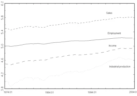
In order to illustrate the practical value of the proposed methods, let us consider the monthly indicators that The Conference Board uses to build the composite coincident indicator of the business cycle in the US. In particular, the empirical analysis concerns the logarithms of Em-ployees on non-agricultural payrolls, Personal income less transfer payments,12 Industrial pro-duction, and Manufacturing and trade sales for the period 1974.1-2003.7. These series are graphed in Figure 1. Although the data are available from 1959.1, only the post first oil-shock period is used because a preliminary application of the test by Bai et al. (1998) revealed that a VAR model of these series is affected by a structural break occurring in the late 1973.
According to the longest significant lag rule, a VAR(6) with a linear trend is fitted to the data. This model seems to appropriately reproduce the dynamic features of the data since the null hypothesis of no residuals autocorrelation is clearly not rejected by both the single-equation and multivariate tests. Table 4 reports the results of the Johansen’s LR tests for cointegration, which suggest the existence of one cointegrating vector.
Table 4
Trace tests for cointegration r = 0 r ≤ 1 r ≤ 2 r ≤ 3 72.33∗∗ 38.26 21.20 9.236 * (**) Significant at the 5% (10%) confidence level
Having fixed r = 1, the presence of the various forms of common cyclical features is scru-tinized. The results, reported in Table 5, indicate s = 1 for the SCCF, WF and PSCCF, and
1 2
Figure 1: The US business cycle coincident indicators
s = 2 for the WFP. Overall, the evidence favors the existence of one unrestricted WFP, and one common feature of a restricted form.
Table 5 Common features tests
s ≥ 1 s ≥ 2 s ≥ 3 s = 4 SCCF 20.20∗∗ 88.70 187.8 495.7 WF 17.14∗∗ 60.24 155.7 421.1 PSCCF 16.25∗∗ 59.74 118.4 257.4 WFP 15.56∗∗ 36.16∗∗ 90.36 207.7
* (**) Significant at the 5% (10%) confidence level
Since the presence of two unrestricted WFP’s and one cointegration vector implies that one PSCCF exists,13 it is of interest to check whether the restricted form of common feature is either a WF or a SCCF. A test for the former hypothesis produces a test statistic equal to 7.64
1 3Indeed, there exists a direction lying in the space spanned by bδ that has a null coefficient for the
with a p−value equal to 0.27, whereas a test for the latter hypothesis produces a test statistic equal to 8.65 with a p−value equal to 0.28. Since the SCCF is nested within the WF, these results put forward the coexistence of one unrestricted WFP and one SCCF. The estimates of the associated common feature vectors are reported in Table 6.14
Table 6
Estimates of the common features relationships SCCF (1, −1.571, 0.423, 0.038)0∆yt
WFP (1, 0.445, −0.668, −0.469)0∆yt+ (0.673, 0.191, 0.031, −0.100)0∆yt−1− 0.004bβ 0 ∗yt−1∗
Remarkably, the model that incorporates the above common features relationships has 52 parameters, whereas the model that only satisfies the SCCF restrictions calls for the estimation of 74 parameters.
5
Conclusions
This paper offers an approach for simultaneously modelling different forms of common cyclical features among I(1) time series. After showing that several existing forms of common features are nested within a new model, namely the weak form of polynomial serial correlation common features, some iterative procedures are proposed for testing and imposing diverse forms of common features to a cointegrated VAR model. The empirical application reveals that the new methods provide a model of the US business cycle indicators that is considerably more parsimonious than those obtained by previous notions of common cyclical features.
References
[1] Ahn, S.K. and G.C. Reinsel (1988), Nested Reduced-Rank Autoregressive Models for Multiple Time Series, Journal of the American Statistical Association, 13, 352-375.
[2] Anderson, T.W. (2002), Canonical Correlation Analysis and Reduced Rank Regression in Autoregressive Models, The Annals of Statistics, 30, 1134—1154
1 4
The switching algorithm was terminated when the relative decrease of det³Σeε
´
become inferior than 0.01%. Overall, seven iterations were needed for numerical convergence.
[3] Bai, J., Lumsdaine, R.L. and J.H. Stock (1998), Testing for and Dating Breaks in Multivariate Time Series, Review of Economic Studies, 65, 395-432.
[4] Beveridge, S. and C.R. Nelson (1981), A New Approach to Decomposition of Eco-nomic Time Series into Permanent and Transitory Components with Particular Attention to Measurement of the Business Cycle, Journal of Monetary Economics, 7, 151-174.
[5] Cubadda, G. (1999), Common Cycles in Seasonal Non-Stationary Time Series, Journal of Applied Econometrics, 14, 273-291.
[6] Cubadda G. (2007), A Reduced Rank Regression Approach to Coincident and Leading Indexes Building, Oxford Bulletin of Economics and Statistics, 69, 271-292.
[7] Cubadda, G. and A. Hecq (2001), On Non-Contemporaneous Short-Run Comove-ments, Economics Letters, 73, 389-397.
[8] Engle, R.F. and C.W.J. Granger (1987), Cointegration and Error Correction: Rep-resentation, Estimation and Testing’, Econometrica, 55, 251-278.
[9] Engle, R.F. and S. Kozicki (1993), Testing for Common Features (with comments), Journal of Business & Economic Statistics, 11, 369-395.
[10] Ericsson, N. (1993), Comment (on Engle and Kozicki, 1993), Journal of Business and Economic Statistics, 11, 380—383.
[11] Haldrup, N., Hylleberg, S., Pons, G., and A. Sansó (2007), Common Periodic Correlation Features and the Interaction of Stocks and Flows in Daily Airport Data, Jour-nal of Business & Economic Statistics, 25, 21-32
[12] Hecq, A., Palm, F.C. and J.P. Urbain (2000), Permanent-Transitory Decomposition in VAR Models with Cointegration and Common Cycles, Oxford Bulletin of Economics & Statistics, 62, 511—532.
[13] Hecq, A., Palm, F.C. and J.P. Urbain (2006), Common Cyclical Features Analysis in VAR Models with Cointegration, Journal of Econometrics, 132, 117-141
[14] Johansen, S. (1995), Identifying Restrictions of Linear Equations with Application to Simultaneous Equations and Cointegration, Journal of Econometrics, 69, 111-132.
[15] Johansen, S. (1996), Likelihood-Based Inference in Cointegrated Vector Autoregressive Models, Oxford University Press, Oxford.
[16] Johansen, S. and K. Juselius (1992), Testing Structural Hypotheses in a Multivariate Cointegration Analysis of the PPP and UIP for UK, Journal of Econometrics, 53, 211-244.
[17] Lucas, R. (1977), Understanding Business Cycles, Carnegie-Rochester. Series on Public Policy, 5, 7-29.
[18] Mizon, G E (1995), A Simple Message for Autocorrelation Correctors: Don’t. Journal of Econometrics, 69, 267-288.
[19] Paruolo, P. (2003), Common dynamics in I(1) systems, Department of Economics, University of Insubria WP, 35.
[20] Paruolo, P. (2006a), Common Trends and Cycles in I(2) VAR Systems, Journal of Econometrics, 132, 143-168 .
[21] Paruolo P. (2006b), The likelihood ratio test for the rank of a cointegration submatrix, Oxford Bulletin of Economics and Statistics, 68, 921—948.
[22] Paruolo P. (2006c), Finite sample comparison of alternative tests on the rank of a cointegration submatrix, paper presented at The 8th workshop of the ERCIM working group on Matrix computation and Statistics, Salerno, September 2006
[23] Proietti, T. (1997), Short-Run Dynamics in Cointegrated Systems, Oxford Bulletin of Economics & Statistics, 59, 405-22.
[24] Reinsel, G.C. and R.P. Velu (1998), Multivariate Reduced-Rank Regression: Theory and Applications, Lecture Notes in Statistics, Springer, New York.
[25] Sargan, J.D. (1983), Identification in Models with Autoregressive Errors. In Studies in Econometrics, Time Series and Multivariate Statistics, S.Karlin, T. Amemiya and L.A. Goodman (eds), Academic Press, New York, 169-205.
[26] Vahid, F. and R.F. Engle (1993), Common Trends and Common Cycles, Journal of Applied Econometrics, 8, 341-360.