UNIVERSITÀ DI PISA
Facoltà di Scienze Matematiche Fisiche e Naturali
Corso di Laurea Specialistica in Scienze Fisiche Anno Accademico 2013/2014
Tesi di Laurea Magistrale
Study on the Performances of a PET
System Used for the Control of the
Dose in Hadrontherapy
Candidato: Relatore:
Contents
Introduction 1
1 Outline of the hadrontherapy 5
1.1 Birth and development of the hadrontherapy . . . 5
1.1.1 Italian facilities for hadrontherapy . . . 9
1.2 Dose monitoring in hadrontherapy . . . 12
2 Physical basis of a PET system 15 2.1 Medical Imaging with Positron Emission Tomography . . . 15
2.1.1 Basic principles of PET . . . 16
2.1.2 Physical limits of the PET imaging . . . 17
2.2 Experimental apparatus of a PET system . . . 21
2.2.1 Properties of the detectors . . . 21
2.2.2 Photomultiplier tube . . . 23
2.2.3 Loss of events in a detector system . . . 25
3 DoPET device 29 3.1 Scintillator detector . . . 29
3.2 Photomultiplier tube . . . 31
3.3 Front-end electronics . . . 32
4 Experimental results about performances of the device 39 4.1 Preliminary work on acquired data . . . 39
4.1.1 Pixel identification . . . 40
4.1.2 Energy calibration . . . 40
4.2 Drift of positions of events . . . 43
4.3 Dead-time . . . 51
4.3.1 Dead-time due to single counts . . . 51
4.3.2 Recovery of coincidence losses . . . 52
4.4 Spatial resolution . . . 58
4.5 Noise Equivalent Count Rate . . . 62
4.5.1 Followed procedure for the study of the NEC curve . . 65
Conclusions 71
Introduction
In this work a positron emission tomograph used for the monitoring of the dose in hadrontherapy has been studied and optimized.
The Positron Emission Tomography (PET) is a medical imaging tech-nique which employs a radiotracer which is injected inside the body of the patient.
The tracer is a β+ emitter; the positron annihilates with an electron of the tissue giving rise to two γ rays emitted back-to-back. The line that connects the two annihilation photons is used to reconstruct the zone where the radiotracer settles.
The PET monitoring in hadrontherapy exploits the same process of the standard PET measuring the activity distribution, with the difference that radionuclides are not injected inside the body, but they are created by nuclear interactions of the heavy ions beam with crossed material.
In this work the performances of a PET hardware equipment, developed at the INFN of Pisa, to monitor the induced activity by an hadron beam interacting with matter will be discussed.
The device is a planar dual-head PET scanner. Each head is composed by four separated detectors consisting of a LYSO matrix of 23 x 23 pixels, a position sensitive photomultiplier tube, the front-end electronics which gives the position and trigger signals sent to the main acquisition board.
In Chapter 1 a brief description of the birth of hadrontherapy1 is given.
In particular, in hadrotherapy heavy particles beams are employed to destroy tumoural masses inside the body, the particles commonly used are protons and carbon ions. They deliver almost all their energy in a narrow peak, whose depth depends upon the energy of ions; thanks to this fact it is possible to diminish the released energy in healthy tissues respect to photons or electrons.
When hadron beam crosses matter it could produce isotopes, as 11C, 13N or 15O, that are β+ emitters; then, after radioactive decay and the
annihilation, they will produce two γ rays, which, once revealed, give the distribution of isotopes and so it is possible to localize where the beam has interacted.
The basic principles of the PET technique are described in Chapter 2. Here the characteristics which concern the photons detection and problems linked to physical limits of devices are discussed.
Successively, the standard components of a PET tomograph are intro-duced, such as: scintillator detectors; photomultiplier tubes and the charac-teristics of the electronics.
The description of the system here characterized is given in Chapter 3. As mentioned above, it consists of a planar double-heads detectors made up of a scintillator LYSO matrix coupled with a photomultiplier tube, it is connected to the front-end electronics which communicates with the main FPGA (Field Programmable Gate Array).
Electronics has already been the object of previous studies, [Ferretti12] and [Sportelli10], for what concerns its upgrade and optimization, then only its last version, which is that used for the presented analysis, will be de-scribed.
The results and the analysis that have been done on this system are presented in Chapter 4.
The work is related to the performances of the device. It has been done according to NEMA Standard publications; this protocol refers to small ani-mals PET scanners, then some of the procedures have been adapted to that particular geometry.
The analysis carried out pertain to the study of various characteristics of the system, like:
• energy resolution;
• dead time of the device, both for single counts and for coincidences; • spatial resolution in different points of the FOV, Field Of View, using
two different point sources; • Noise Equivalent Count Rate.
Before those analysis it has been examined a particular behaviour ob-served concerning the pixel maps, namely that the pixel positions change depending on the rate of the source, then it should be necessary a new cali-bration at every activity level.
The method employed to correct maps will be described at the beginning of Chapter 4; the idea behind the correction was that to find a function that describes the changing of the maps with respect to rate, such as to implement it in the reconstruction model, avoiding in this way the wrong attribution of the events.
CHAPTER
1
Outline of the hadrontherapy
In this chapter the developments of hadrontherapy is briefly introduced, touching on the different types of accelerators employed for therapies, re-ferring to facilities built in Italy.
Subsequently, the importance of the dose monitoring in hadrontherapy is described; in particular the application of the PET imaging, in dose moni-toring, is presented.
1.1
Birth and development of the
hadronther-apy
The choice to use ionizing radiation against tumoural tissues is related to the possibility to control the energy released in matter by particles.
It is possible to control the dose1 released by radiation and the depth
reached by particles only setting their type and energy.
Furthermore, therapy with radiation beams is not invasive as traditional surgery2 and it could develop even thanks to the fact that sick cells are more
1The dose is defined as the mean energy transferred in a volume of mass dm: D = dhEi dm ,
and it is measured in gray (Gy).
2However, even if the number of tumours treated with particle beams is increasing,
susceptible to damage of the DNA and because of their lower capability to restore it compared with healthy ones, that are hit too.
After the decision to treat a tissue with radiation the treatment plan has to be decided. The treatment plan is decided according to algorithms, like Monte Carlo simulations, that calculate the optimal dose distribution to deliver to the volume of interest, to that purpose some data are needed, like: planning target volume (PTV, that is the volume to irradiate); beam energies; cross sections of the particles; geometry of the accelerator; and details about patient’s anatomy.
A few of these informations about the patient are taken from other imag-ing techniques, like CT from which material densities and heterogeneities are recovered, to correct range uncertainties and so to calculate the best possible release of the dose.
However, there are other sources of uncertainty, like: patient set-up; pa-tient’s movement, as that due to breathing; wrong evaluation of dose; and wrong dose delivery. For all these reasons the treatment of a tumour with radiation is not always possible.
It must be considered that it is not possible to treat all types of tumours with ionizing radiation; in fact the decision about the treatment of a car-cinoma with it is made considering the separation of the TCP and NTCP curves, that respectively are: the Tumour Control Probability, and the
Nor-mal Tissue Complication Probability. Those probabilities are calculated using
models that assess: type of radiation, treated volume, damages, organ mo-tion, setup errors and others parameters that will not be discussed here but are available in [Warkentin04].
An example of the the trend of the two probabilities is shown in figure 1.1. The more the curves are separated, the better is the therapeutic window, and so the treatment could be favourable.
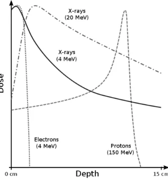
The types of radiation employed in radiotherapy are: photons of energy up to 25 MeV; electrons up to 30 MeV; protons from tens to 250 MeV; and heavy ions up to 400 MeV/u.
All these particles have different curves of release of the dose due to their different nature, as shown qualitatively in figure 1.2. As evident from the figure, photons release a part of their energy on the surface of the irradiated tissue and then the exponential absorption follows; so they could damage healthy tissues or organs placed behind the treated zone.
Figure 1.1: Examples of the Tumour Control and Normal Tissue Complica-tion probabilities as funcComplica-tion of the dose released [Naqa12].
On the contrary, protons and heavy ions deposit their energy in a narrow region, known as Bragg peak, and they release a small fraction of their energy before and after that, preserving healthy organs (called Organ At Risk, OAR) that eventually could be near the tumour.
Therefore, the importance of heavy particles like protons and ions lies in their way to interact with matter. In fact, referring to the Bethe-Block equation, they are weakly influenced by Coulomb interaction with electrons (because of their bigger mass), and so their path is approximately linear, until they reach the final point of the range, corresponding to Bragg peak, where they deliver all the energy.
Furthermore, it has to be considered that protons and heavy ions are more biologically effective than photons (in fact ions break the double strand of cellular DNA more easily than photons, decreasing the probability that cells would be able to repair it [Nunes13]); so it is required lower dose to obtain the same damage.
From the curve of the dose released by protons in figure 1.2, it is evident that the Bragg peak due to a monoenergetic proton beam is too narrow to irradiate the entire volume of a tumoural mass. Then it is necessary to broaden the peak; in fact the profile of the beam that reaches the patient is modulated to obtain a conformal shape to the target region. The peak
Figure 1.2: The figure shows the curves of the release of dose of different types of particles of various energies.
so enlarged is called Spread-Out Bragg Peak (SOBP), and it is displayed in figure 1.3.
From the figure it is possible to appreciate that the broadening entails an increase of the dose delivered along the path, but, considering the dose released to healthy tissues, the SOBP is still better than photons to treat deep tumours.
The SOBP could be obtained either passively, i.e. with layers of material placed between the exit of the beam and the target, or actively, that is varying the energy of the protons.
Further details about the experimental setup to broaden the Bragg peak are available in [Paganetti05].
For all these reasons hadrontherapy developed as a technique to treat tumours in oncologic surgery, thanks to the damage ions cause to cell and the more effective treatment to radioresistant tumours.
Figure 1.3: Example of the dose released by superimposed proton beams of different energies used to treat a cancerous tissue. It is also displayed the dose profile of a photons beam necessary to deliver the same energy in the deepest part of the tumour (Courtesy of: Mark Filipak).
1.1.1
Italian facilities for hadrontherapy
Hadrontherapy could grown thanks to developments of particle accelerators. However, today, qualified structures for hadrontherapy are not diffused as much as that for radiotherapy, because the facilities are still very expensive; on the contrary, X-ray tubes and linear accelerators for electrons are more common for their lower cost.
In the early stages of its application, in about the ’30s, the therapy was based on the use of fast neutrons, but they were abandoned because of the non-optimal dose distribution3.
Proton therapy developed from about 1945 thanks to studies about the profile of the energy released by these particle in matter. Since then hadron-therapy grew even more and a lot of facilities have been built. A more de-tailed history about the birth and development of hadrontherapy is available in [Amaldi10].
Today, in Italy, two structures for hadrontherapy are in operation: the CNAO (Centro Nazionale Adroterapia Oncologica) in Pavia; and CATANA (Centro di AdroTerapia e Applicazioni Nucleari Avanzate) the center to treat the ocular melanoma with protons beam, in Catania.
The center of CNAO is provided with a synchrotron and three treatment rooms, the facility was planned to treat tumours with both carbon ions and proton beams. A plant of the CNAO facility is reported below, in figure 1.4.
Figure 1.4: Schematic view of the facility for hadrontherapy in Pavia. There are visible the synchrotron and the three treatment rooms, in one of which the beam arrives vertically besides horizontally.
The financing of this project arrived in 2000 and the construction started in 2005, during 2010 the qualification of the two beam types was done and in 2011 treatments began. The main kinds of diseases treated at CNAO are: head and neck tumours; eye melanoma; bone sarcomas and paraspinal tumours.
A detailed description about the CNAO facility is available in [Rossi11]. The center of CATANA, instead, is provided of a cyclotron where are accelerated only protons. The facility is specialized in the treatment of ocular melanoma and rare ocular diseases; the size of the beam, reduced to 50 mm diameter with a collimator, is suitable to treat these kind of tumours.
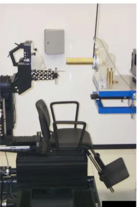
The facility is operative from 2002 and a picture of the treatment room at CATANA facility is shown in figure 1.5.
Before the beam reaches the patient, positioned on the chair, it must cross some elements that modulate its shape, in particular: a range shifter
Figure 1.5: Picture of the positioning chair and the last collimator from which the proton beam exits, inside the treatment room at CATANA facility.
to obtain the necessary energy to reach the tumour; a PMMA modulator to form the SOBP; two monitor chambers to control on-line the intensity of beam; and the final collimator of 50 mm diameter [Cirrone04].
Table 1.1 summarizes characteristics of CATANA and CNAO facilities.
Facility Accelerator Start treatments Particle Max. En. (MeV)
CNAO Synchrotron 2011 p, C-ions 250, 400/u
CATANA Cyclotron 2002 p 62
Table 1.1: The table shows the main characteristics of hadrontherapy struc-tures in Italy.
1.2
Dose monitoring in hadrontherapy
The growth of the hadrontherapy and its increasing application to treat tu-mours lead inevitably to the need to have a control as precise as possible of the dose delivered to tissues crossed by radiation, with the goal to hit primarily sick ones.
To this purpose it is necessary to measure exactly the range of hadrons and the distribution of the energy released along their path, that depends upon the materials intercepted.
There are different methods to measure proton range, as described in detail in [Knopf13]: directly or indirectly; and online or offline. The former circumstances refer to the case if the range is obtained directly or from an-other signal, the latter refer to the fact if the estimation is made during the treatment or after that.
One of the indirect methods uses the Positron Emission Tomography approach, and it could be made both online and offline.
This is an indirect procedure because it makes use of photons that are originated by the annihilation of positrons emitted by radionuclides, like11C
or 15O, produced by nuclear reactions between protons and crossed matter.
These isotopes have short half lives, and they decay emitting a positron, which will annihilate with an electron of the surrounding matter, giving two gamma rays back-to-back, as will be described in detail in section 2.1.1. The data so acquired give the profile of the activity.
Three different types of data acquisitions with a PET device can be dis-tinguished [Shakirin11]: in-beam; in-room; and off-line PET. In the first case the device acquires while the irradiation is taking place; in the second case the measure is made right after the irradiation, and it requires a PET tomograph near the treatment room where the patient is positioned.
The off-beam measurements are made placing the patient in a PET scan-ner away from the treatment room, and it is done in a time from 10 to 30 minutes, so only information from isotopes created by radiation with longer half-life is recorded, as example, referring to table 2.1, it is not possible to gain informations from the decay of Oxygen.
Actually, the in-beam dose monitoring is not easy to put in practice, because, during beam extraction, the high amount of events that hit the detector could paralyze it4.
Furthermore, in-beam monitoring gives data corrupted by the high num-ber of random coincidences, that cannot be subtracted with standard tech-niques. However, systems based on synchronization with the radio frequency of synchrotrons have been developed, they acquire data during pauses from beam extraction; differently for cyclotrons it is not possible to gain useful in-beam data [Crespo05].
A device designed to monitor in-beam activity induced by a proton beam could not be a conventional circular PET scanner, but it requires a specific geometry. The first strategy adopted has been that to use a double-head geometry scanner, because a full ring one may collide with the patient or the beam [Shakirin09]. However, recently it has been developed a project called OpenPET, in Japan, which makes use of a full-ring PET scanner to provide PET scanning during radiotherapy, the open space accessible to the beam is due to fact that the ring has a slant angle respect to axial direction [Tashima12].
The use of a dual-head scanner brings also to artefacts in image recon-struction. Those artefacts are due to low statistics and to the geometry of the detector, in fact it is not possible to use analytical algorithms, because all angular projections are not available, as required by the Filtered-Back
Projection algorithm. Hence, only iterative algorithms are usable, increasing
computing time.
The first prototype of in-beam PET scanner was built at the carbon ion therapy facility at GSI Helmholtzzentrum für Schwerionenforschung (Center for heavy ions research), Darmstadt, Germany. It is composed by two de-tector heads, assembled in the treatment room and positioned to form two circular arcs opposite one another.
Differently, the device characterized in this work is a planar double-head PET system, and its detailed description will be given in the third chapter.
can increase if a big amount of events reaches the detector, causing the interruption of data acquisition; a description of this type of detector will be discussed in chapter 2.
CHAPTER
2
Physical basis of a PET system
In this chapter the physical principles of the PET imaging are introduced. Then both the physical and practical limits related to the PET imaging are discussed.
The generic experimental apparatus of a PET tomograph is here de-scribed, in particular the characteristics of the scintillation crystal and the photomultiplier tube.
2.1
Medical Imaging with Positron Emission
Tomography
The various techniques of medical imaging use the different ways of radiation to interact with matter.
A first differentiation can be done between transmission imaging and the emission one. The CT technique and the radiography, for instance, belong to the former category, in this case the source of radiation is placed outside the body; on the contrary, for the emission imaging a radioactive isotope is injected inside the body and then it concentrates in different zones and organs depending on metabolism; so, reconstructing the activity of the isotope, it is seen where it localized; for this reason it is called also functional imaging. The PET (Positron Emission Tomography) and SPECT (Single-Photon Emission
Isotope Half life (min)
11C 20.4
13N 9.96
15O 2.03
18F 109.8
Table 2.1: The table lists the isotopes used for the Positron Emission To-mography and their half lives expressed in minutes.
Computed Tomography) are part of this kind of imaging.
2.1.1
Basic principles of PET
The Positron Emission Tomography is a medical imaging technique used to obtain informations about a living body.
PET imaging is based on the β+ decay of radioactive isotopes. The β+ decay is described by:
A ZX = A Z−1Y + β ++ ν e (2.1)
the energy released in the reaction (neglecting the recoil of the father nucleus) is shared out between the positron and the electron neutrino according to a certain distribution probability.
The most common isotopes used for the PET imaging are shown in table 2.1.
Today, the most used isotope is the18F , linked with a molecule of glucose
to form the18F-FDG (fluorodeoxyglucose). The reason for the choice of this particular molecule is due to its capability to reach tissues, like cancerous ones, that have an anomalous need of glucose, and its decay properties. In fact, 18F is a β+-emitter with half life of about 109 minutes, this period is
enough to allow its diffusion inside of the body, and it is even enough brief not to leave an activity inside the patient for too long.
As soon as the radiotracer is injected inside the body the emitted positrons, after they have lost all their energy, annihilate with an electron of the tissue. The annihilation produces two γ rays of energy of 511 keV (which is the rest mass of both the particles involved in the process), that, in first approxima-tion, are emitted back-to-back, which means that the angle between them is
180◦1.
The PET image is obtained by reconstructing the position where electron and positron annihilate, as an estimation of the side where the radiotracer has been accumulated. The difference between the reconstructed position and the location where the tracer settles is due to positron range and other factors, see equation 2.3.
The technique used to do this is to place the patient inside a ring of detectors and collect the γ rays originated by the annihilation processes. The line that joins two annihilation photons is called LOR (Line Of Response); by reconstructing all the LORs an evaluation about the position and the concentration of the radiotracer is obtained.
2.1.2
Physical limits of the PET imaging
During an acquisition of a PET signal there are two main problems related to it; firstly there is the capability to discern if two events belong to the same annihilation process, and than there is the capability to estimate the position where the reaction took place.
Coincidences in PET
The PET imaging is based on the possibility to detect two photons that interact at the same time in detectors placed the opposite one another.
However, the simultaneous detection of the two γ rays is affected by some factors, for example the delay due to the electronics or the annihilation doesn’t occur at the center of the field of view of the tomograph. So it is essential to specify a time interval called coincidence window.
The coincidence window can be defined as the time within that two γ rays, of energy of 511 keV, could be considered pertaining to the same annihilation event. The typical value of a timing window for a clinical PET tomograph is 10 ns, but in case of preclinical scanners (scanners that are used for research on small animals, and so with a smaller gantry) it can be reduced to values less than 5 ns.
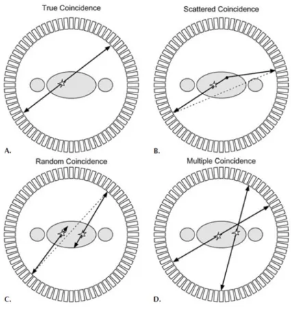
Referring to a generic PET tomograph, it is possible to identify different types of coincidences, as reported in figure 2.1.
1To be more precise the angle between the two γ rays is 180◦±0.25◦, because sometimes
Figure 2.1: The figure shows the different types of coincidences that could be registered during a PET acquisition.
The true coincidences are defined as two events, originated by a single annihilation process, that are revealed within the timing window and that could be considered approximately collinear, meaning that none of the two has done a scattering event.
The scattered coincidences are due to the events that have done a Comp-ton scattering with the surrounding atoms (being them part of the body, the air, or the table where the patient is positioned); the random ones are caused by events that are independent from each other, but they get into the same timing window, so they could be considered as events of a single annihilation. The multiple coincidences occur when three or more occurrences are reg-istered simultaneously2, so it is impossible to detect what is the true pair of
2As previously outlined, the mention to coincidences is always in reference to the events
photons originated by the annihilation process.
As it is evident, all but true coincidences are useless to reconstruct the correct position of the annihilation without ambiguities. So it is necessary to discriminate true events from the other ones.
An event that has done one or more Compton interactions should be excluded because the photon hasn’t the original direction anymore and the reconstructed LOR would be incorrect. The photon, because of the inter-action, loses a part of its energy, so it can be distinguished increasing the energy resolution of detectors, and excluding it from data used for the recon-struction.
The number Cr of the random coincidences relies on the width of the
coincidence window and on the activity of the source. This means that increasing the activity of the source and the value of τ , unavoidably the number of randoms increases too.
To discard random coincidences two different methods can be used: the
delayed window technique and the single rates method. The delayed
win-dow technique consists on the measure of events that fall inside the timing window, so they will be the sum of true coincidences and random ones. Sub-sequently the events that occur after a time t τ (whose choice could be
t ≈ 10τ ) are recorded and they are certainly uncorrelated. Then this number
of events is subtracted from that inside the timing window, obtaining true coincidences.
The second method uses the following formula to estimate the number of the random coincidences:
Cr = 2 · Sd1· Sd2· τ (2.2)
being: τ the coincidence window; Sd1 and Sd2 the single rates registered by
the two detectors.
Spatial resolution
In a PET tomograph there are many effects that contribute to the worsening of the spatial resolution of the entire system.
The sum of the terms that provide the broadening of the Full Width at Half Maximum (FWHM) of the spatial resolution is reported below:
F W HM = 1.2 v u u t d 2 !2 + b2+ (0.0022D)2+ r2+ p2. (2.3)
Referring to equation 2.3, each parameter is defined as follows [Belcari06]: • 1.2 is a factor due to the reconstruction;
• d is the width of pixels of the detector;
• b is called coding error, it is originated from the fact that the number of crystals and the number of photodetectors could not be the same, so there is an uncertainty in the attribution of the position of every event; • D is the diameter of the tomograph, and the numerical factor in front
of it is obtained from numerical calculations and approximations; • r is a value linked with both the source dimensions and the positron
range, in fact, as shown in figure 2.2, the positron doesn’t annihilate as soon as it is produced, but after it has travelled for a certain range;
Figure 2.2: The figure represents the positron emission of a radionuclide and the production of two photons of energy of 511 keV, after the annihilation with an electron.
• p is the parallax error; it is due to the fact that the interaction of the photon on the crystal could take place at various depths, but the event is attributed at the surface of the crystal as shown in figure 2.3. This error can be calculated with formula 2.4 and the farthest the annihilation happens from the center of the tomograph, the more it is relevant:
p = α√ r
where: r is the distance between the center and the annihilation point;
R is the radius of the tomograph and α is a numerical parameter which
hinges on the type and the thickness of the detector employed.
Perceived LOR
True LOR
Figure 2.3: The figure shows the error in the reconstruction of the LORs due to the fact that the photon could interact at different depths in the crystal.
2.2
Experimental apparatus of a PET system
The generic experimental setup that constitutes a PET tomograph consists in a ring of detectors coupled with photomultiplier tubes, which in turn are connected to the electronic system of data acquisition.
2.2.1
Properties of the detectors
Different types of detectors could be used to build a PET system, in partic-ular it can be used: gas chambers, semiconductor detectors and scintillation detectors3.
3Only the physical effects that are the basis of the scintillation process will be described
Scintillation detectors can be made both of inorganic or organic materials, but the use of the former prevails upon the other ones in PET systems.
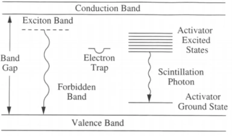
The scintillation material has a band structure; in particular it can be distinguished the valence band and the conduction band, separated by an energy gap. Introducing impurities of another element, called activator, other states can be created between the bands, as shown in figure 2.4. This is made to change the band structure of the crystal, making easier the emission of visible light during de-excitation processes.
The scintillation process is schematized in figure 2.4.
Figure 2.4: Scheme of the scintillation process in an inorganic crystal in which impurities are present.
When photons hit the crystal they deposit all or part of their energy by creating hole-electron pairs. So, the electron is free to drift and it can fall inside an excited site of the activator (because the presence of the activator introduces possible states within the forbidden gap); subsequently, it returns in the valence band emitting a photon in the visible range. The emission time of the scintillation light depends on the half life of the excited state involved4.
Therefore, in a scintillation crystal, one of the most important properties is its capability to convert the deposited energy in visible light; an approx-imated number of the visible photons produced for 1 MeV of energy of the most common crystal is given in table 2.2. In addition to this the crystal
4Generally there are also other types of emission of energy, but they are not radiative
ρ (g/cm3) λem (nm) Decay Time (ns) L.Y. (photons/MeV) n NaI(Tl) 3.67 415 230 38000 1.85 CsI(Tl) 4.51 540 680(64%), 3340(36%) 65000 1.80 BGO 7.13 480 300 8200 2.15 LSO 7.4 420 47 25000 1.82 YAP 5.37 370 27 18000 1.95 LYSO(Ce) 7.3 428 50 28000 1.82
Table 2.2: The table shows the main properties of some scintillation crystals, in particular: density; emission wavelength; decay time; light yield; and the refractive index [Knoll00].
should have a linear response to the deposited energy to better discriminate events.
There are other important characteristics of a scintillation crystal that have to be taken into account in its choice; some of them are listed in table 2.2. Especially, the material should have a short decay time to be able to discriminate each pulse at high rates; and it should have high density to detect even high energy radiation: moreover the crystal has to be transparent to its scintillation light, to not reabsorb it.
Another fundamental property is the energy resolution; it is defined as:
R = F W HM H0
(2.5) where the FWHM is the Full Width at Half Maximum of the photoelectric peak and H0 is the channel in correspondence of the peak. Obviously it is
better to have a low value of R, as it is evident in figure 2.5.
The scintillation light is emitted isotropically; for this reason it is nec-essary that the crystals have reflective walls to not disperse the light and to direct it toward the surface of the photomultiplier tube. So, the crystal should have the refractive index as close as possible to the one of the glass (n ≈ 1.5) to allow an efficient diffusion of the light through the photocathode of the PMT.
2.2.2
Photomultiplier tube
Scintillator crystals are optically coupled with photomultiplier tubes (PMTs) that amplify the signal exiting from the crystal and detect the position where
Figure 2.5: Example of different responses of two detectors to the same source. Even if the position of the peaks is the same, the detector with
R = 40% has worse performances.
visible photons interact.
The scheme of the structure of a typical PMT is shown in figure 3.3.
Figure 2.6: Scheme of a photomultiplier tube.
As it is possible to see from the scheme, when a photon hurts the scin-tillator it produces scintillation photons, whose fraction reaches the photo-cathode of the PMT emitting an electron, which is accelerated toward the first dynode; by colliding with it, other electrons are ejected, which in turn will reach the further dynode, and so on up to the last one, where the charge is collected and sent to the electronic system of data acquisition.
The amount of the secondary electrons emitted depends on the energy of the primary ones, so, if it is not enough, the electrons would be unable to go beyond the valence band reaching the conduction one and finally exiting from the material. At this purpose it is important the choice of the materials with which the photocathode is constructed.
This one can be made with different materials, in particular metals or semiconductors; the former have a potential barrier between 4 eV and 5 eV, the latter between 1.5 and 2 eV. The latter are more widely used because of the quantum efficiency, defined as the ratio between the number of photo-electrons produced and the number of incident photons on the photocathode, is bigger for semiconductor materials.
It is possible to give an estimate of the gain of a photomultiplier tube with the expression:
G = α · δN (2.6)
being: α the number of the electrons exiting from the photocathode; δ the number of the electrons produced by the first dynode and N the number of stages of the tube. As an example, with 9 stages, α = 1 and δ = 5 it is obtained G = 106.
It must be considered that the use of semiconductor materials, albeit it makes possible to obtain an higher sensitivity to slower electrons and an higher quantum efficiency, it brings to a greater noise due to the thermal current. Some sources of noise are: leakage current; field emission, which takes place when an electron exits from a dynode because of its thermal energy and it is accelerated by the high electric field; electrons deviating from their trajectory and hitting the envelope causing scintillation electrons; cosmic rays and natural radioactivity.
2.2.3
Loss of events in a detector system
The loss of events in a detector depends upon different factors like: reabsorp-tion of the scintillareabsorp-tion light inside the crystal; scattering events; interacreabsorp-tion probability, linked with the depth of the crystal; and dead time.
As mentioned above the detector itself could absorb its scintillation light, losing some events.
Scattered events are those that have made inelastic interactions with mat-ter and they have lost part of their energy, then those events are not
consid-ered in image reconstruction5.
The interaction probability could be approximated as P = eLd, being: d the depth of the pixel and L the attenuation length of the material; the value of L varies with the energy of the incident photon but a mean value could be useful to have an idea about the fraction of lost photons.
The dead time is the time interval during which the system is not able to register an event. It is not linked with the crystal but it depends principally on the electronics.
It is necessary a certain time, for a given system, to register an occurred event. It is possible to discern two different types of systems: the paralysable one and the non-paralysable one.
Figure 2.7: The figure shows schematically the process of event recording for both models of detectors, the paralysable and the non-paralysable one [Rizzi10].
The former case is when the system, during the elaboration of an event, is still able to register another one, as schematized in figure 2.7; in this case the time of elaboration data increases and, if the activity of the source is sufficiently high, elaboration time increases because of the high number of events and the system can paralyse.
For a paralysable model detector, the equation for the dead time is:
m = n · e−nτ (2.7)
where n is the true rate of the source, m is the acquired rate and τ is the dead time. It can be notice that it is not analytically solvable so the value
5To be precise the energy window of the events used for the reconstruction comes from
Figure 2.8: The figure displays the trend of the acquired rate depending on the true rate of the source for a paralysable and a non-paralysable model of detector [Rizzi10].
of the dead time must be extracted from a fit.
On the contrary, if a system is non-paralysable it is not able to discern an event while it is still elaborating a previous one, so the electronics won’t be paralysed, but all the events that fall in that period get lost.
In this second case it is possible to determine the acquired rate depending on the true one as:
m = n
1 − nτ. (2.8)
However, if the rate is low, m can be approximated with n(1 − nτ ) in both formulas, and it is evident that the two systems behave in the same way, as it is qualitatively displayed in figure 2.8.
CHAPTER
3
DoPET device
In this chapter the instrumentation of the double-head PET scanner to con-trol the precision of hadrontherapy treatments is described.
In particular a brief description of the scintillator crystal, the photomul-tiplier tube and the front-end electronics is given.
The DoPET system is a double-head device, whose heads, positioned opposite one another, can be fixed at 14, 20 or 30 centimeters of distance between them. The two detectors are then connected to power supplies devices and to acquisition electronics.
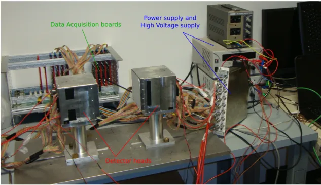
In figure 3.1 the system assembled is displayed.
Inside both of the two heads there are four scintillating crystals, each of them is coupled with a photomultiplier tube, powered by high voltage supply, which is in turn connected to the front-end electronics. The sensible surface of the heads is about 10 x 10 cm2
The electronics is then connected with cables to: power supply; DAQ (Data Acquisition boards); and trigger system.
3.1
Scintillator detector
The type of crystal used in this device is an inorganic scintillator detector. The material used is LYSO:Ce; the crystal matrix is composed of 23 x 23
Detector heads
Data Acquisition boards High Voltage supplyPower supply and
Figure 3.1: The picture shows the dual-head detector. There are visible the two heads; the support, where they are fixed at a distance of 20 cm, that is the distance at which all data have been taken; the power supply modules and the acquisition electronics.
pixels of volume: 1.9 x 1.9 x 16 mm3.
A picture the crystal is shown in figure 3.2.
Figure 3.2: Scintillator matrix of 23x23 pixels of LYSO material. Lutetium is composed by two isotopes: the non radioactive 175Lu; and
the radioactive 176Lu in abundance 2.59%. The isotope 176Lu decays, with
half-life of 3.6 · 1010 years, emitting an electron, with mean energy of 420
keV, and three gamma rays whose energies are: 307 keV, 202 keV and 88 keV [Yamamoto05].
It has to be taken into account that, if an electron is revealed simultane-ously with a gamma ray, they can produce a coincidence event; so, when the characterization of the scanner is performed it must be taken into account the intrinsic single and true rates, as recommended by the Standard NEMA protocol [NEMA08].
3.2
Photomultiplier tube
The photomultiplier tubes used here are the Hamamatsu H8500, whose pic-ture is reported in figure 3.3.
Figure 3.3: Position-sensitive photomultiplier tube, model: H8500, Hama-matsu Photonics.
The PMT has a sensible area of 49 x 49 mm, that fits with the dimensions of the crystal, it has 12 stages of metal channel dynodes coupled with a 64 channel matrix type multianodes. Anodes are connected with 16 rows, eight are used to reconstruct the position in the x direction, the others eight for the position in the y direction. Further characteristics about the H8500 tube are available on the datasheet [Hamamatsu].
The cathode is made with a bialkaline material and the entrance window is done with borosilicate glass. The first choice has been made to improve the sensitivity of the cathode and the second one is due to the will to reduce background counts. A document, released by the Hamamatsu Photonics, where it is possible to find other characteristics of a photomultiplier tubes is available in [Hamamatsu06].
3.3
Front-end electronics
The photomultiplier tube is connected to two boards, precisely to the Sym-metric Charge Division (SCD) and subsequently to the Pulse Shape Pream-plifier (PSP) and the Constant Fraction Discriminator (CFD) boards. A picture of one of the assembled modules that composes the two heads is shown in figure 3.4. Figure 3.5 displays the arrangement of the four modules inside one of the heads and there are even reported values of the distances between crystals.
Crystal
Photomultiplier Tube
Symmetric Charge Division board Pulse Shape Preamplifier and Constant Fraction Discriminator
Figure 3.4: The picture shows one of the eight modules which compose the DoPET’s heads. There are visible the scintillator crystal connected to the photomultiplier tube, and the front-end electronics: the Symmetric Charge Division; the Pulse Shape Preamplifier and Constant Fraction Discriminator board.
The first board is the SCD, it is directly connected with the tube H8500. It reads the signals coming from the anodes of the phototube; and reduces
6 mm 3 mm B3 B1 B4 B2 104 mm 46 mm z = 0 y = 0
Figure 3.5: Position of modules inside one of the two heads that constitute the detector. On figure the distances between crystals are reported, in particular it is possible to notice the central gap of 6 millimeters due to boards of the scintillator matrices.
them from 64 to 8 + 8 and finally to 2 + 2 with a resistive network; the four signals let then return to the position of the interaction [Olcott05].
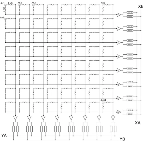
A scheme of the resistive grid is visible in figure 3.6; the signal from each anode is split in two parts, one for X axis and one for Y axis from two resistors of the value of 1 kΩ, and, as it is evident, the values collected for the X direction and the Y one are independent from each other.
The 16 values are then sent to the PSP board and amplified. Here each one of these is divided by two resistors (RA and RB for every signal), whose
Figure 3.6: The figure illustrates the resistive grid connected to the anodes of the photomultiplier tube and the operation made by the PSP circuit. The grey squares represent the anodes (some of them are omitted for simplicity). All the resistors of the grid have the same value (1 kΩ), and every anode is connected to two of them, one for the X direction and the other for the Y direction. Each of the 8 + 8 signals crosses two resistors of different value (calculated as in equation 3.2), reducing the number of signals to 2. Resistors for the valuation of YA and YB have the same values of that for the X direction.
Rn,A = Rmax n (3.1) Rn,B = Rmax N − n + 1 (3.2)
where Rmax = 5.11 kΩ, N in the number of the signal in one direction, so,
in this case N = 8, and n is the index of the signal. Hence the values of the resistors are chosen in such a way that they vary linearly increasing n.
Finally the signals are sent to the Data Acquisition boards (DAQ) and the position of interaction of a photon is calculated from the 4 values of the voltage collected with the formulas [Belcari07]:
Xposition = XA− XB XA+ XB Yposition = YA− YB YA+ YB . (3.3)
The board where it is integrated the PSP contains even the CFD. The Constant Fraction Discriminator serves to extract the timing signal from the last dynode of the PSPMT. One of the methods to discern an event could be that to use a fixed threshold; so, an event is recorded when this threshold is overtaken. However, in this way, signals cross the threshold depending on their amplitude and rise time.
Employing a constant fraction discriminator the trigger signal activates as soon as the signal exceeds a fraction of its amplitude.
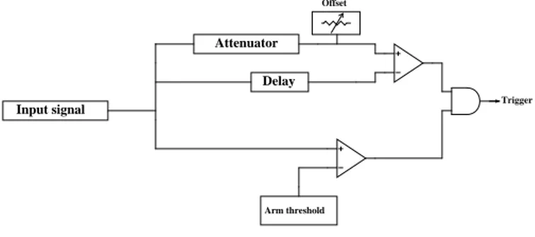
An illustrative scheme of the operation of the CFD is shown in figure 3.7.
Input signal Delay Arm threshold Trigger Offset Attenuator
Figure 3.7: The figure shows schematically the stages of the CFD. As it is shown in the scheme, at the arrival of a signal from the last dynode this is duplicated and sent in three different lines: the signal in the first one is
attenuated at about the 14% and it must overcome an offset, whose function is to avoid that the comparator gives a signal corresponding to noise; a delay of ∆t1 is applied to the second one; the third line, before the signal would
be transmitted to a flip-flop that will generate the trigger signal, is sent to a comparator ad it is compared with a threshold (called arm), the level of this one in chosen as a compromise between low values, that let to have a big amount of counts, and high ones that reduce the dead-time and decrease noise, but at the same time they could lead to the loss of true counts.
The delayed and attenuate signals enter in a comparator, it gives a signal that starts when the amplitude of the delayed signal overcomes that of the attenuated one and so it is sent to the flip-flop.
The reset signal of the flip-flop is connected to the exit of the comparator with the arm threshold and maintains the high logic value as default; the clock signal is given by the comparator between the attenuated and the delayed signals and it is set to low logic value.
If the reset signal leads up to 0 and clock reaches the logic value 1, the ris-ing edge of the trigger signal is generated. The exit of the flip-flop maintains the high logic value until the reset signal comes back to 1.
In table 3.1 are shown some of the values of the components and thresh-olds employed in the CFD circuit.
Parameter Value
Offset 40 mV
Mean Aplitude of input signal 150 mV
∆t 3 ns
Arm threshold 50 mV
Attenuation 14%
Table 3.1: The table lists values used in the CFD circuit. All values had been set taking into account to have a probability of 99.7% to reject noise signals.
After the front-end electronics, located inside each of the two opposite heads, the signals are carried to the Data Acquisition boards (DAQ), that
1The value of the delay is chosen to be less than the time required to the pulse to reach
are plugged on the principal board, called mother-board, and they talk with the main FPGA.
CHAPTER
4
Experimental results about performances of the device
In this chapter the analysis and the results performed on the DoPET system is described.
In the first part, the work done before the reconstruction and the analysis of the images are presented. After that, the results, and the way how they are obtained, about the features of the system, are listed and commented. In particular results are shown about: the recovery of counts from dead-time correction; the spatial resolution and the study of the signal to noise ratio.
The studies that have been made refer to the Standard NEMA Protocol [NEMA08] and for each analysis the method employed is briefly described.
All data sets analysed in this chapter were acquired with the two heads placed at a distance of 20 cm one from the other, and a coincidence time window of 3 ns was always used.
4.1
Preliminary work on acquired data
The characterized device is used for the reconstruction of the dose in hadron-therapy, so it must be as compact and portable as possible, because, to make possible various types of measures, it is led from a facility to another, like: INFN laboratories in Pisa; CNR (Consiglio Nazionale delle Ricerche) in Pisa; CATANA facility in Catania; and CNAO facility in Pavia.
For every data taking it is necessary to perform a pixel identification to attribute the events precisely and an energy calibration to convert ADC (Analogue to Digital Converter) channels into energy channels.
4.1.1
Pixel identification
The first necessary step before the reconstruction of an image is the pixel
identification. It consists in the assignment of the acquired events to the pixel
of the crystal matrix. To do that, a dedicated software has been developed, but a control of the pixels is required on the edge because the software is not always able to distinguish them.
The resulting pattern of the pixel map in shown in figure 4.1(a). The reason of that scheme is due to the coupling between the crystal matrix and PMT; a sketch of this coupling is reported in figure 4.1(b).
(a) (b)
Figure 4.1: The figure shows the resulting pixel map of a module when irradiated with 511 keV γ rays. On the right it is shown the coupling between the LYSO matrix and the PSPMT H8500. As visible, only pixels that have the same distance from four anodes are correctly reconstructed, but those which fall near the center of a single anode drift beside the anode itself.
4.1.2
Energy calibration
The acquisition for the energy calibration is made with a planar source placed in the middle of the two heads, it has the same extension of the detector surface to enlighten all the FOV with the same intensity.
The energy calibration is necessary because the ADC channels associated to every pixels must be converted in energy units to indicate the energy of photons which have interacted with the detector.
Every pixel has its own efficiency and then a different response to the same incident energy. Therefore the position of the peak which corresponds to 511 keV changes considering each element.
The gain of the pixels is calculated by inverting the formula:
CkeV(i) = α(i) · CADC(i) (4.1)
where CkeV(i) corresponds to channel in energy units, α(i) is the efficiency
of the pixel i and CADC(i) is the raw ADC channel, then:
α(i) = 511 CADC(i)
(4.2) where the position of the ADC channel is chosen as the mean of a Gaussian fit on the peak of 511 keV. Figure 4.2 shows a typical spectrum of the events collected by a pixel.
Figure 4.2: The figure shows the distribution of events by every ADC channel collected by a pixel and the Gaussian fit superimposed on the peak corre-sponding to 511 keV.
After the procedure of assignment of the peak at 511 keV, all the events accumulate in a module are summed together obtaining the total energy spectrum from which it is possible to calculate the energy resolution.
Values of the energy resolution were obtained making a Gaussian fit on the peak around the channel which corresponds to the energy of 511 keV. The fit doesn’t consider all the points of the photopeak because the shape of the spectrum was not exactly Gaussian. In particular, fifty points around the maximum value were taken, this choice was made considering the R2
parameter returned by Matlab1, that is a measure of the goodness of fit, and maintaining fixed this number of points R2 remained greater than 0.99 for
all spectra.
The reason of the non-Gaussian shape of the photopeak had been studied in [Bonifacio10], here an optical model for the coupling between a LYSO matrix and a photomultiplier tube is proposed and it is demonstrated that the tail at high energies is due to optical interactions inside the crystal.
Figure 4.3 shows the energy spectra obtained with the calibration.
0 200 400 600 800 1000 1200 1400 1600 1800 2000 0 0.5 1 1.5 2 2.5 3x 10 5
Energy channels [keV]
Counts
Energy spectra of single modules
A1 A2 A3 A4 B1 B2 B3 B4
Figure 4.3: Energy spectra of all modules of the device.
Table 4.1 lists results obtained about the energy resolution of all modules. Values about the energy resolution of the entire system are calculated from those obtained for single modules and are listed below in table 4.2.
1The R2 parameter is calculated as: R2= 1 − Σ(yi−fi)2
(yi−ym), where yi are the data, ymis
Module µ [keV] FWHM Energy Resolution A1 508.8 103.5 20.3 % A2 509.6 102.6 20.1 % A3 508.3 111.0 21.8 % A4 508.3 107.9 21.2 % B1 509.5 98.6 19.3 % B2 509.9 102.3 20.0 % B3 508.9 104.3 20.5 % B4 509.3 99.2 19.5 %
Table 4.1: Values of the energy resolution of all the eight crystals and of the entire system calculated as the mean value of those of all modules; µ is the mean of the Gaussian fit made on channels that correspond to the photopeak and the FWHM is calculated from the value of the standard deviation as:
F W HM = 2.35 · σ.
µ [keV] FWHM Energy Resolution
509.1 ± 0.6 103.6 ± 4.1 20.3 ± 0.8 %
Table 4.2: Energy resolution of the DoPET system.
4.2
Drift of positions of events
A first observed problem is the variability of the maps with varying the activity of the source; it has been noticed that maps, obtained with the acquisition used for the calibration, didn’t fit with the positions of the pixels acquired with a different rate of the source.
This difficulty has been resolved changing the value of the pedestal coor-dinates, to avoid the pixel identification every time the source rate changes. The name pedestal refers to an acquisition made with the high voltage modules turned off. Hence, the pedestal file contains unreal events, but they are required to remove the baseline so as to correctly reconstruct the position of the events. As described in section 3.3, positions of interaction are calculated with Anger’s logic, but it must be pointed out that the four
position coordinates are calculated as:
XA= XE,A− XP,A; XB = XE,B− XP,B
YA = YE,A− YP,A; YB = YE,B− YP,B
where XE, YE are the coordinates of the event and XP, YP are values
con-tained in the pedestal file2.
This fact, i.e., the widening or the narrowing of the maps depending on rate, is not due to the pedestal, this being an acquisition with the high voltage supply switched off. An high rate of the source could cause a raising of the signal’s baseline due to the sum of the tails of events, as schematically shown in figure 4.4. The correction is made by altering artificially pedestal coordinates because it is the easier way to correct maps.
V(t)
t
Figure 4.4: Example of the baseline fluctuations due to pulses pile-up. As an example, maps before and after the correction are shown in figure 4.5.
The steps followed to investigate the variation of the pixel maps are listed below:
• the pixel identification is done using the acquisition with a planar source (in this case it was done using a source of FDG with nominal activity equal to 17.5 MBq);
• different acquisitions with different activity were superimposed on maps to visualize how much they differed from those of the calibration; • pedestal coordinates of every module, inside the calibration file, were
multiplied by a factor adapting them to the considered acquisition.
2The detailed implementation of the correction with pedestal coordinates is available
(a) High rate map superimposed on the original calibration
(b) High rate map superimposed on the corrected calibration
(c) Low rate map superimposed on the original calibration
(d) Low rate map superimposed on the corrected calibration
Figure 4.5: Example of maps obtained with higher and lower rate of the source compared with that used to do the calibration is reported. Figure (a) shows the pixel map of the calibration superimposed on a higher rate acquisition; (b) shows the corrected map to fit on the registered events; (c) is the calibration superimposed on a lower rate acquisition; and (d) is the modified map that fits over the events.
Henceforth, it will be referred to the first calibration made with the planar source as “planar calibration”, and to the calibration with changed pedestal values as “corrected calibration”.
In principle, each module has its own response. In fact, counts recorded by each of them were different, and then each pedestal has to be multiplied by a different factor.
The study of this effect and the validation of a method that describes the trend of the corrections are useful to implement the improvement inside the reconstruction software, in such a way it takes into account the changing of position of pixels.
The method consists in extracting parameters from a function which fits with factors k used to modify pedestal coordinates depending on the sum of recorded counts.
The function that has been used is a quadratic polynomial curve, it hasn’t a physical meaning, but the reason of this choice resides in the fact that it was required a compromise between the correctness of the model and the easiness of implementation3 inside the reconstruction software.
As mentioned above, considering the fact that every tube has its own gain, eight polynomials (one for each module) were found, but to simplify the implementation of the method it was made a fit on all values of the k factors. The resulting plot in shown on figure 4.6, the value of the reduced
χ2 is of 0.37, a such low value could be due to the fact that the uncertainties
on k were taken as 0.1, because this value was the finest possible tuning of multiplying factors.
Parameters obtained from the parabolic fit are:
k = 1.08 · 10−13c2− 6.21 · 10−7c + 1.37. (4.3) The following maps show the events of a low activity source as they fit with the calibration made with the planar source (figure 4.5 (a)) and the corrected calibration using others low rate data (figure 4.5 (b)).
The same acquisition as it fits with the calibration made with the planar source (figure 4.7 (a)) and the corrected calibration using others low rate data (figure 4.7 (b)).
Counts recorded by the two considered acquisitions are:
3A cubic polynomial curve was also tested, but since the goodness parameter given by
the fit had the same value of that returned by quadratic fit, it was decided to use the curve with lower number of parameters.
0 0.5 1 1.5 2 2.5 x 10⁶ 0.4 0.5 0.6 0.7 0.8 0.9 1 1.1 1.2 1.3 1.4 Counts k factor
Figure 4.6: The plot shows the k factors depending on counts collected by single modules and the parabolic fit (red line) made on them.
• 5.8 · 104 counts for the acquisition used to correct the calibration;
• 3.78 · 104 counts of the acquisition superimposed on the corrected
cali-bration.
The value of the pedestal used in the corrected calibration is k = 1.3 and, referring to figure 4.6, counts of the acquisition used to validate the calibration are in agreement with those corresponding to that factor.
Figure 4.8 shows reconstructions of a capillary source, filled with high activity, made with two different calibration archives: that made with the planar source, and that corrected. Similarly, figure 4.9 displays a low activ-ity cylindrical source. The contrast in the images has been opportunately regulated to enhance the differences between the two images.
The analysis of the uniformity of the activity inside phantoms has been made to quantify the differences between the images reconstructed with the two different calibration archives.
The measures have been done referring to the Standard NEMA for what concerns the uniformity measure; there are reported: the mean value of the
(a) (b)
Figure 4.7: The maps refer to the same statistics visualized on two different calibrations of the same module. Figure (a) is the acquisition superimposed on planar calibration; figure (b) is the same acquisition superimposed on corrected calibration.
(a) (b)
Figure 4.8: Results of the reconstruction of a phantom with the calibration made with the planar acquisition (a), and with the correct calibration (b).
grey level inside the considered ROI; the maximum and minimum values inside the same region; and the percentage standard deviation.
(a) (b)
Figure 4.9: Results of the reconstruction of a cylindrical phantom with the calibration made with the planar acquisition (a), and with a corrected cali-bration made on a different acquisition (b).
However, it was not possible to apply step by step the protocol because the used phantoms had a different geometry; in particular, the measure has been done on a single slice of the reconstructed image without making the sum on a volume in order to avoid considering regions with no activity.
The %ST D is defined as:
%ST D = ST D
M ean· 100. (4.4)
Comparisons between the two reconstructions of the capillary and of the cylinder placed in various positions are listed in tables 4.3 and 4.4.
From values listed in table 4.4 it is possible to notice that the percentage standard deviation has lower values in the image with the corrected maps, that means a decrease in fluctuations of pixel values and so a greater uni-formity in the region filled with the activity, this trend is underlined even by the fact that the difference between the maximum and minimum values decreses inside the considered ROI.
Regarding measures made on the capillary reconstructions, table 4.3, the improvement is less marked; probably it is due to the particular geometry of the source, whereby the recovery of the events on edge pixel (because the
Calibration Mean Max Min STD % STD
Planar 1.20 105 1.45 105 1.03 105 7.0 104 5.8%
Corrected 1.35 105 1.47 105 1.21 105 5.4 104 4.0%
Table 4.3: Values extracted from the same ROI in the images of the capillary source. In particular the selected region was in the yz plan and the selection included only 53 pixels, because it is a measure about the uniformity, so it must be sure that the activity is the same along all selection.
Calibration Mean Max Min STD %STD
Position in FOV: x = 0; y = 0; z = −25 Planar 29.14 50.18 17.24 6.48 22 % Corrected 26.61 46.17 20.28 5.43 20 % Position in FOV: x = 0; y = 0; z = −15 Planar 28.62 46.28 15.85 5.99 21 % Corrected 28.06 41.98 19.49 4.78 17 % Position in FOV: x = 0; y = 0; z = 5 Planar 22.08 33.80 12.81 4.44 20 % Corrected 21.51 30.08 13.35 3.19 14 % Position in FOV: x = 0; y = 0; z = 35 Planar 20.45 32.44 10.28 4.44 21 % Corrected 19.98 27.98 14.07 2.94 14 % Position in FOV: x = 0; y = −26; z = −25 Planar 12.02 22.68 6.61 3.04 25 % Corrected 12.45 21.34 7.67 2.65 21 % Position in FOV: x = 0; y = −26; z = 0 Planar 13.32 24.41 7.68 3.45 26 % Corrected 13.83 24.23 9.30 2.93 21 %
Table 4.4: Values extracted from reconstructions of the cylindrical phantom reconstructed with the two different calibration archives, in different positions of the FOV. The phantom was filled with a solution of18F-FDG, the selection,
in the yz plan, includes 270 pixels and it is about the 75% of the entire surface as required by the Standard NEMA. Positions recorded refer to the center of cylinder.
adjustment of maps operates mainly on them) is not so necessary as for the case with an extended source.
The following steps summarize the correction that will be implemented inside the reconstruction software to restore the maps depending on counts recorded by every module:
• for every frame the number of measured single counts are read;
• the corrective k factor is extracted from the function in figure 4.6 and it will be multiplied to pedestal coordinates;
• the corrected pedestal coordinates are subtracted from the coordinates of events, as described in section 3.3;
• the positions of events are reconstructed using the new pedestal coor-dinates.
4.3
Dead-time
In this section the results about the dead-time of the DoPET system will be shown. The first analysis concerns the study of the dead-time due to single counts collected by every module of the scanner, subsequently the results about the losses of coincidences due to the dead-time are shown as well as the way to correct this losses inside the reconstruction software.
4.3.1
Dead-time due to single counts
The acquisition for the evaluation of dead-time should be done with a source of known activity and it should be long enough until the activity recorded by the scanner coincides with the intrinsic radioactivity4.
The acquisition lasted nearly twenty hours; it was done at the CNR of Pisa with a radioactive source of 18F-FDG with initial nominal activity of
62.9 MBq.
4This request comes from the standard NEMA and it refers to scanner made with
ra-dioactive materials; for others detectors the acquisition should last until the ratio between random rate and true rate is less than 1%.
The first analysis concerns the measure of dead-time of each module of the system using single counts. It is done using a script composed by two sections: the first one estimates the initial activity of the source and the values of the background counts, owed to the radioactivity of the Lutetium contained in the LYSO, using the function:
N (t) = N0· e−
t
τ + b (4.5)
where N (t) are counts varying during acquisition time, N0 is the number of
counts at the beginning of the acquisition, τ is the half life of the radionuclide and b represents the number of the intrinsic radioactivity, N0and b are leaved
as parameters of the fit.
Then, parameters returned by the fit are used to estimate the activity of the source and the rate recorded is plotted as a function of that expected theoretically and it is fitted with the formula that describes a paralysable model of detector (as previously mentioned in section 2.2.3).
This last fit returns the value of the dead-time of detector. An example of the trend of acquired counts depending on expected ones is shown in figure 4.10.
From the figure 4.10 it is evident that for low rates of the source, the behaviour of all modules coincides with that of a paralysable detector, but at high activity counts fall abruptly and the fit detaches from data. Referring to the fit on plot, and even considering the trend for a paralysable model of detector in figure 2.8, it seems that the number of acquired counts should start to fall at higher rates rather than to those obtained.
The falling of counts is imputable to a non-ideal behaviour of the CFD caused by pile-up events, at high source rates, that paralyse the front-end electronics. Therefore only acquired data before paralysation of the system are those used for the analysis and they are described by the paralysable model of detector as found in literature.
The values of dead-time for single counts of every module that composes the two heads are listed in table 4.5.
4.3.2
Recovery of coincidence losses
The acquisition software produces two different files: the statistics file and the events file. Those files, in addition to other informations, provides
![Figure 1.1: Examples of the Tumour Control and Normal Tissue Complica- Complica-tion probabilities as funcComplica-tion of the dose released [Naqa12].](https://thumb-eu.123doks.com/thumbv2/123dokorg/8021529.121968/11.892.217.600.186.485/figure-examples-control-complica-complica-probabilities-funccomplica-released.webp)
![Table 2.2: The table shows the main properties of some scintillation crystals, in particular: density; emission wavelength; decay time; light yield; and the refractive index [Knoll00].](https://thumb-eu.123doks.com/thumbv2/123dokorg/8021529.121968/27.892.122.761.190.339/properties-scintillation-crystals-particular-density-emission-wavelength-refractive.webp)
![Figure 2.8: The figure displays the trend of the acquired rate depending on the true rate of the source for a paralysable and a non-paralysable model of detector [Rizzi10].](https://thumb-eu.123doks.com/thumbv2/123dokorg/8021529.121968/31.892.213.609.192.431/figure-displays-acquired-depending-paralysable-paralysable-detector-rizzi.webp)