On the Non-Inflationary effects
of Long-Term Unemployment Reductions
†Walter Paternesi Meloni,
*Davide Romaniello
**and Antonella Stirati
***Working Paper No. 156
April 9, 2021
ABSTRACT
The paper critically examines the New Keynesian explanation of hysteresis based on the role of long-term unemployment. We first examine its analytical foundations, according to which rehiring long-term unemployed individuals would not be possible without accelerating inflation. Then we empirically assess its validity along two lines of inquiry. First, we investigate the reversibility of long-term unemployment. Then we focus on episodes of sustained long-term unemployment reductions to check for inflationary effects. Specifically, in a panel of 25 OECD countries (from 1983 to 2016), we verify by means of local projections whether they are associated with inflationary pressures in a subsequent five-year window. Two main results emerge: i) the evolution of the long-term unemployment rate is almost completely synchronous with the dynamics of the total unemployment rate, both during downswings and upswings; ii) we do not find indications of accelerating or persistently higher inflation during and after episodes of strong declines in the long-term unemployment rate, even when they occur in country-years in which the actual unemployment rate was estimated to be below a conventionally estimated Non-Accelerating Inflation Rate of Unemployment (NAIRU). Our results call into question the role of long-term
† A preliminary version of this work has been presented at the 17th STOREP Conference (October 2020) and the 4th
ASTRIL International Conference (December 2020). We thank for their comments Prof. Luca Fantacci and all the participants to our sessions. The usual disclaimer applies.
* Research Fellow, Department of Economics, Roma Tre University
** Research Fellow, Department of Economic and Social Sciences, University Cattolica del Sacro Cuore
unemployment in causing hysteresis and provide support to policy implications that are at variance with the conventional wisdom that regards the NAIRU as an inflationary barrier.
https://doi.org/10.36687/inetwp156
Keywords: Hysteresis; Long-term Unemployment; NAIRU; Inflation; Labor Market.
“There is no sign that the pool of supposedly less employable long-term unemployed people, which has so preoccupied economists and governments, ever existed”
(Webster, 2005)
“We have not yet seen clear indications that the short-term unemployed are finding it increasingly easier to find work relative to the long-term unemployed”
(Yellen, 2014)
1. Introduction and background
The post-Great Financial Crisis period has featured, particularly in Europe, persistently higher levels of unemployment, as well as lower growth rates and an estimated potential path far below its pre-crisis trend. Many authors have regarded these developments as not independent of the recession. Such prolonged effects in terms of economic activity and increased unemployment, however, are in contrast with standard macroeconomic models, according to which Central banks can continually keep the economy close to its potential level by means of interest rate management. This newer thinking has two weighty implications. First it casts severe doubt on the legitimacy of
New Consensus macroeconomics, whose main feature is confidence in monetary policy’s ability
to reduce output volatility and ensure stable and lasting growth in capitalist economies (Goodfriend, 2007). It also favors the revival of the theme of hysteresis, both in the unemployment rate and output level (Blanchard and Summers, 1986; Ball, 2014; Blanchard et al., 2015; Blanchard, 2018; Girardi et al., 2020).1 Hysteresis is generally meant to imply that by increasing
the actual unemployment rate significantly, a deep recession may also cause a change in the equilibrium unemployment rate or the Non-Accelerating Inflation Rate of Unemployment (NAIRU) and, consequently, in potential output. In essence, this approach admits the possibility that a cyclical fall in economic activity may have persistent effects on macroeconomic outcomes. In addition to persistently higher unemployment rates, what animated the rediscovery of hysteresis was the absence of the deflationary pressure that standard macroeconomic models would have required to restore the pre-crisis equilibrium: this phenomenon has been termed missing deflation, and it further testifies to a puzzle concerning the unemployment-inflation link (Yellen, 2014). Hysteresis, and in particular the missing deflation side of the tale, has been explained in connection with the presumed worsening of long-term unemployment. It is within this line of inquiry that we wish to situate our paper, and we particularly aim at assessing this explanation at the empirical level. According to the just-mentioned interpretation of hysteresis, higher levels of the NAIRU resulting from an increase in long-term unemployment would boost the inflationary risk of expansionary policies. Such a higher risk would depend on the fact that labor demand would primarily involve short-term unemployed individuals who would be able to bargain for substantial
1 The New Consensus developed during the so-called period of Great Moderation, that is, between 1985 and the Great
Recession. In that context, the concept of hysteresis was almost totally neglected by academic research. As Blanchard (2018) has pointed out, over time, as the so-called Great Moderation took place from the mid-1980s up to about 2007,
wage increases, owing to the inability of the long-term unemployed to actually compete for the jobs. Indeed, according to this literature, all long-term unemployed people can be regarded as bad
inflation fighters. This, it is claimed, depends on the fact that they suffer from skill deterioration
and/or detachment from the labor market, two conditions that would relegate them outside the realm of wage negotiations and thus make them non-competitors with regard to the other workers. As a consequence, their status is considered hardly reversible without engendering sizeable inflationary pressures. Thus, we have on one side an expansionary policy aimed at reabsorbing unemployment that would hardly be effective in reducing its long-term component; on the other side, the presence of a relatively large pool of long-term unemployed individuals would make overall unemployment less effective in weakening wage inflation, thus providing an explanation for the missing deflation. It is clear that crucial in this line of reasoning is the assumption of
asymmetry between total and long-term unemployment. In fact, this interpretation of hysteresis
would predict that when total unemployment falls (i.e., during phases of economic recovery), its long-term component would not fall in the same proportion. In turn, this implies that attempts to reduce long-term unemployment by means of expansionary policies, even if successful, would require paying a price in terms of higher or accelerating inflation rates.
Starting from this, we put under empirical scrutiny the validity of the New Keynesian (NK) assumption of irreversibility of long-term unemployment. Predominantly, we do so by investigating the evolution of long-term unemployment and aggregate unemployment in a panel of 25 mature OECD countries to verify whether irreversibility is supported at the empirical level. Secondly, we present an econometric analysis aimed at verifying whether inflationary surges are likely to occur during and after episodes of strong reduction of the long-term unemployment rate and in a subset of such episodes when, according to official estimates, the unemployment rate was already below the conventionally accepted NAIRU. To do so, we employ local projections, as initially introduced in Jordà (2005) and recently used in Girardi et al. (2020), to assess the dynamic impact in terms of inflation of 78 (58 in the subset) cases of sharp, long-term unemployment reductions that occurred between 1983 and 2016.
The rest of the paper proceeds as follows. In Section 2, we present in some detail the NK explanation of hysteresis caused by long-term unemployment. Section 3 deals with the inquiry regarding the relationship between long-term and overall unemployment. In Section 4, we focus on the effects in terms of inflation of sustained reductions in the long-term unemployment rate. Section 5 concludes and draws some implications for the current policy debates on unemployment and hysteresis.
2. The role of long-term unemployment in New Keynesian models
2.1 Long-term unemployed as detached from the labor market and bad inflation fighters Three main explanations for hysteresis can be found in the literature.2 The first focuses on the
interaction of labor market institutions and shocks in causing unemployment persistence and relies on insider-outsider models (Blanchard and Summers, 1986; Lindbeck and Snower, 1986). The second focuses on the impact of aggregate demand on capital formation, and it is based on the negative effects of reduced investment on capital stock and productivity (Haltmaier, 2012; Gordon, 1995; Rowthorn, 1995, 1999). The third one dwells on the role of the long-term unemployed. In
this paper, we focus on the latter, which with a certain degree of generality can be summarized as follows. The NK explanation of hysteresis postulates that long-term unemployed individuals lose employability and detach from the labor force. As a result, they cease to exert downward pressure on wages, to the point that they are considered ‘bad inflation fighters’ and responsible for the ‘missing deflation’. Hence, a larger pool of long-term unemployed people would lead to an increase in the NAIRU (Rusticelli, 2015; Mathy, 2016), and therefore to a decline in potential output.3
According to the existing literature, the long-term unemployed would have fewer chances of being reemployed than the short-term unemployed – and then would not contribute to pushing down inflation – for reasons involving both labor demand and labor supply. Usually, the socio-economic literature identifies this phenomenon with the term duration (or state) dependence. The intuition behind this is rather simple: the longer the duration of unemployment, the lower the probability of being rehired (Layard et al., 1991; Bean, 1994; Blanchard and Diamond, 1994; Dosi et al., 2016). From the supply side, the duration of unemployment would be positively associated with discouragement in job searching (Phelps, 1972; Heap, 1980; Johansen, 1982; Devine and Kiefer, 1991; Schmitt and Wadsworth, 1993; Bean, 1994; Krueger and Mueller, 2012) and with the depreciation of human capital (Pissarides, 1992; Ljungqvist and Sargent, 1998). It has also been argued that a lower effort in job searching may depend on unemployment benefits (Ljungqvist and Sargent, 1998; Bassanini and Duval, 2006) and that detachment from the labor market would be higher in cases where they are notably generous (Guichard and Rusticelli, 2010). It should be noted, however, that in order to determine an increase in the NAIRU, discouraged and marginalized workers should not completely leave the labor market but remain unemployed, that is, actively seeking jobs; in the event that discouragement pushes them to leave the labor force, the NAIRU would actually decrease.
From the demand-side, employers are said to discriminate among candidates depending on the duration of their status of unemployment (Acemoglu, 1995): specifically, businesses would be able to rank job applications based on the spell of unemployment (Lockwood, 1991; Blanchard and Diamond, 1994) and would be less willing to hire long-term unemployed people (Ghayad, 2013; Kroft et al., 2016).4 This reluctance is called the stigma effect, and it would exist as long as
employers believe that long-term unemployed individuals are characterized by lower productivity than short-term unemployed individuals (Røed, 1997; Abraham et al., 2016). In turn, according to some contributions, this would depend on the fact that a longer time in unemployment signals the existence of individual characteristics that make them scarcely employable (unobservable
3 The concept of NAIRU has been criticized along different lines by a variety of works belonging to the broadly
defined post-Keynesian tradition. Among these, the reader can refer to Arestis and Sawyer (2005), Storm and
Naastepad (2007) and Lang and Setterfield (2020). Stockhammer (2008)traces a series of specific characteristics of
the NAIRU and evaluates them in alternative theoretical frameworks. A recent policy brief by Blanchard (2016), based on an earlier paper (Blanchard et al., 2015), raised a number of interesting points concerning the NAIRU and the Phillips Curve. A partial reconsideration of the ‘natural rate’ of unemployment also emerges in Blanchard (2018).
4 In this regard, some authors attributed the shift to the right of the Beveridge curve to the role of long-term
unemployment (Bouvet, 2012; Ghayad and Dickens, 2012). Other works have criticized this view along different lines of inquiry (Elsby et al., 2010; Diamond and Şahin, 2015; Mathy, 2016).
heterogeneity), so that some scholars have labeled them as bad apples (Imbens and Lynch, 2006;
Kroft et al., 2016).
Although both explanations are currently subject to debate and not wholly supported by evidence,5
the explanation of hysteresis relies on the assumption that long-term unemployed people are on the margins of the labor force, and therefore they are considered as exerting feeble (downward) pressure on wage dynamics (Ball, 1999; Krueger et al., 2014). Accordingly, an increase in the pool of long-term unemployed would not weaken the wage claims by the ‘insiders’.
In this respect, the work by Llaudes (2005) is rather clear. In his words, ‘long-term unemployed,
as outsiders, have little influence on the wage bargaining process, while the insiders, the employed or newly unemployed, have the ability to impose their wage aspirations’ (p. 11). This view, too,
has been questioned at the empirical level (Speigner, 2014). However, it is still at the core of the standard NK formalization of hysteresis based on the role of the long-term unemployed.
2.2 Long-term unemployment and hysteresis in the 3-equation model
To understand how the NK approach formally incorporates the possibility of hysteresis in the labor market, let us refer to a standard macroeconomic textbook presentation (cf. Carlin and Soskice, 2006, 2014). According to this, central banks manage the policy interest rate to constantly keep the economy close to its potential level.6 This also implies equilibrium in the labor market: by
affecting the level of activity, the monetary policy aims at closing the unemployment gap, that is, the difference between the actual and the ‘natural’ rate of unemployment or the NAIRU. As in the short run, due to the existence of wage and price rigidities, an exogenous shock in aggregate demand may affect both output and employment, the actual unemployment rate may deviate from the NAIRU, and consequently, the inflation rate would start to change. Therefore, the Central bank would intervene by adjusting the policy interest rate in order to achieve its inflation target.7
Generally, inflation falls when there is slack in the labor market (that is, a positive unemployment gap) and grows when the labor market is tight (a negative unemployment gap). Accordingly, in the medium to long run, this framework is compatible with a vertical Phillips curve (Blanchard, 2016).
5 Some criticisms have been advanced on different grounds, to the point that some very influential scholars have
partially revised their perception of the role of the long-term unemployed (Blanchard, 2006; Blanchard and Katz, 1997). For instance, even supporting the notion that time out of work leads to skill decay, Edin and Gustavsson (2008)
do not disregard the possibility of reverse causation (that is, whether negative trends in skills lead to unemployment).
Moreover, a variety of works have criticized the role of unemployment benefits in affecting labor market outcomes (Baker et al., 2005; Armingeon and Baccaro, 2012; Stockhammer and Sturn, 2012; Aleksynska, 2014; Boone et al., 2016).
6 A clarification is needed here. Within the NK framework, potential output is defined as the maximum level of output
achievable with the maximum utilization of production factors (generally, labor and capital) consistent with existing market imperfections and a stable inflation rate. Potential GDP is essential in policy making because Central banks use the difference between actual and potential GDP (i.e., the output gap) to determine whether the economy needs more or less monetary stimulus.
7 In this respect, the following quote by Carlin and Soskice (2014) is quite evocative: ‘What is the central bank trying
to achieve? It is assumed that its aim is to use monetary policy to stabilize the economy, which means keeping the economy close to equilibrium output and keeping inflation close to its targeted rate’ (p. 89).
Technically, the monetary authority makes use of a monetary policy rule, an equation describing the behavior of the Central bank in terms of the output gap (or equivalently in terms of the unemployment gap) and the deviation of the actual inflation rate from its target.8 In this way,
monetary authorities operate to preserve the economy around its potential level and keep the pace of inflation constant. We can see it in the so-called 3-equation model (Carlin and Soskice, 2006, 2014), which includes:
i) a standard IS curve (Equation 1) representing the demand side of the economy, in which output ( ) is a positive function of autonomous expenditure ( ) and a negative function of the real interest rate ( );
ii) an accelerationist Phillips curve (Equation 2), representing the supply side of the economy, where the actual inflation rate is a function of the output gap ; explicitly, only when the output gap is closed, the actual inflation rate ( ) is equal to the expected inflation rate ( ); iii) a monetary policy rule (Equation 3), representing the behavior of the Central bank; here, the output gap relates to the deviation between the actual inflation rate and its target , and the parameter indicates to what extent the Central bank is inflation-adverse.9
(1)
(2)
(3)
To capture the role of hysteresis in increasing the inflationary risk of an expansionary policy, we combine the above-sketched 3-equation model with a standard NK model of the labor market. Instead of the neoclassical model which considers labor demand and labor supply curves, the NK model of the labor market includes a price-setting curve ( ) and a wage-setting curve ( ). The two curves represent the behavior of employers and workers, respectively, in a non-competitive labor market (Carlin and Soskice, 2014; Blanchard, 2017).
On the one side, the curve represents the level of real wages, expressed as the ratio between nominal wage ( ) and expected prices ( ) desired by the employees. Here, the real wage is positively related to total employment ( ) and its intercept is determined by a parameter ( ).10 The
latter represents all the wage push factors able to increase the bargaining power of workers (e.g., labor market institutions, unemployment benefits and trade union influence) and, in this sense, they are viewed as market stickiness. According to the formalization provided by literature (Layard
8 The best-known approach is the Taylor rule (Taylor, 1993), a guideline for Central banks in setting the policy interest
rate to achieve an equilibrium real interest rate. For a deeper discussion on the behavior of the monetary authority, see, among others, Blinder (2000), Taylor (2000), Setterfield (2004) and Carlin and Soskice (2006). For a critical view of the estimates of the equilibrium (natural) rate of interest and the stance of monetary policy, see Levrero (2019).
9 More precisely, the higher the aversion to inflation, the higher the loss of output and employment that the Central
bank will be willing to accept in order to avoid inflation surges.
10 Unlike the formulation by Carlin and Soskice (2014) adopted here, in Blanchard (2017), the schedule is
downward-shaped as it considers unemployment instead of employment. However, this does not affect the general line of reasoning as for a given labor force, unemployment is the difference between active population and employment.
et al., 1991; Carlin and Soskice, 2014), the parameter , together with the aforementioned institutions operating in favor of workers, also captures the role of long-term unemployment in wage-setting. The reason behind this interpretation is consistent with the NK explanation of hysteresis: the effect of long-term unemployment on the wage-setting curve is analogous to the role played by pro-worker labor market institutions.11
On the other side, the curve represents the real wage determined by the price-setting rule followed by enterprises. As is standard in macroeconomics textbooks (Carlin and Soskice, 2014; Blanchard, 2017), for the sake of simplicity, we assume a flat schedule.
As far as the formalization of the model is concerned, Equation (4) indicates how workers set their request for nominal wage on the basis of an expected level of prices. In parallel, Equation 5 shows how enterprises set prices, and hence the actual real wage, by adding a fixed mark-up ( ) to a given labor productivity ( ). Only when the labor market is in equilibrium (i.e., only when the actual unemployment rate is equal to the NAIRU), the actual real wage set by employers ( ) is the same desired by workers ( ), and the expected and actual price levels coincide.
(4)
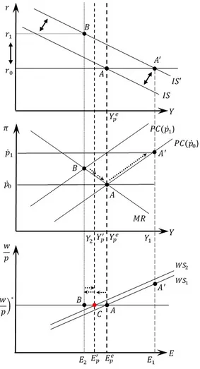
(5). This toolbox helps us to understand how hysteresis works within a NK macroeconomic model and, more importantly, what its implications are for the dynamics of the inflation rate. A complete picture is provided in Figure 1, which combines three graphs: the upper one is the IS curve; in the middle, we find the Phillips curve ( ) and the monetary rule ( ); and the lower graph represents the - labor market. Starting from a general equilibrium (both in goods and in labor markets) depicted by point , let us suppose that an unexpected increase in autonomous consumption (i.e., an increase in ) will shift the IS curve to the right (from to ). For the same real interest rate ( ), the economy will move from to , a situation in which income ( ), employment ( and the inflation rate ( are higher than their equilibrium values ( , and , respectively). Moreover, we see that is not on the curve: with higher than , the short-run will shift up. In this situation, if the Central bank wants to bring the system back towards its initial equilibrium ( ), it has to implement a restrictive policy by increasing the monetary interest rate. After the monetary tightening, the economy will move from to , a point that lies on the , where income is and where the inflation rate is lower than . Accordingly, the short-run
will also shift down. The attempt by the Central bank to dampen the inflation rate below would require the actual income to drop below its potential level ( ). What happens after this drop would depend on the presence or absence of hysteresis.
11 As explained in Section 2.1, a higher pool of long-term unemployed people will reinforce the power of workers
involved in the wage negations, inasmuch as they are less employable and, therefore, they will not depress wage inflation (non-inflationary fighters). This recalls the functioning of the insider-outsider models, as already discussed with reference to Llaudes (2005, p. 11).
If hysteresis is not at work, the short-run Phillips curve will progressively shift down until it reaches its initial position: accordingly, the economy will converge to the initial equilibrium ( ). If hysteresis is at work, the greater the Central bank-induced recession, the more long-term unemployment will increase, and the more significant the increase in the NAIRU. Indeed, once long-term unemployment increases, the curve will shift up (from to ), and a new equilibrium will be determined. Putting it differently, the economic system starts moving from to : nevertheless, due to hysteresis, the adjustment stops at , that is, in a new equilibrium with a higher unemployment rate – which in the graph is represented by lower employment ( ) – and a lower potential output ( ). Thus, the unemployment gap is smaller than in the case without hysteresis, owing to the upward shift of the NAIRU that moves it closer to the actual unemployment rate.12 As a result, the threat of inflationary consequences of expansive
demand-side policy increases. The inflationary risk is higher as the increased labor demand resulting from an expansion would primarily be addressed to the short-term unemployed. The latter (as the insiders in insider-outsider models) are the only fraction of the unemployed that has a role in wage negotiations, and this is likely to cause accelerating inflation (Llaudes, 2005, p. 11). According to this model, therefore, accelerating inflation is a necessary result of demand-side policies implemented to fight unemployment as a whole, including its long-term component.13
As mentioned at the beginning of the paper, with these models we face an asymmetry: the presence of a sizeable pool of long-term unemployed people would not weaken wage inflation following a recession, and at the same time, an expansionary policy aimed at reabsorbing unemployment as a whole would push it up. But this looks like a blind alley for full employment policies and motivates us to further investigate at the empirical level the relationships between total unemployment, long-term unemployment and inflation.
3. Unemployment and its long-term component: an explorative inquiry
In the class of models described in the previous section, the increase in long-term unemployment generally experienced after a recession would cause an increase in the NAIRU. Accordingly, the inflationary potential of demand-side expansionary policies aimed at recovering earlier output and unemployment would be high. To inquire in this line of reasoning, we should prima facie investigate whether higher long-term unemployment tends to persist during phases of economic recovery (i.e., when the total unemployment falls). Secondly, we should verify if, as predicted by the models, accelerating inflation would take place in a context of decreasing long-term unemployment, and particularly so if the economy features a null or negative unemployment gap. This section deals with the first step of the empirical analysis, as after looking at some explorative
12 As noted in Martin et al. (2015), after the Great Recession, there is no sign of convergence of the actual
unemployment rate (or actual income) towards the NAIRU (or potential output). On the contrary, they argue that ‘in
contrast to the typical assumption that output grows rapidly after recessions to close the output gap, the gap is also closed through revisions to potential output’ (p. 11).
13 Very clearly, Rudebusch and Williams (2014) state: ‘When the short-term unemployment share was at a historic
low, the optimal monetary policy would allow inflation to rise well above levels implied by the standard model and indeed to overshoot the inflation target for a time’ (p. 6).
evidence we delve deeper into the relationship between long-term unemployment and total unemployment.
The prediction of the hysteresis models under scrutiny is that on the one hand, when total unemployment falls, long-term unemployed people tend to remain in their status of unemployed. This implies a minor role of long-term unemployed people in wage-setting, to the point that if their weight is sizeable, a lower-than-necessary (to reduce unemployment) decrease in the real wage would be observed. In other words, the sacrifice in terms of persistent unemployment to achieve a stable inflation rate would be higher. Quite evocative, in this respect, is the statement by Machin and Manning (1999) that ‘long-term unemployment has been argued to be a cause of high
unemployment itself’ (p. 3087).
Such a view is crucially grounded on the assumption that an asymmetrical relationship between total unemployment and long-term unemployment holds. Some works, to which we will refer below, have already cast unsettling light on this hypothesis. However, before we move to this, some discussion is needed about how best to measure long-term unemployment and its relationship to total unemployment. In the literature, two different measures are alternatively used to assess the magnitude of long-term unemployment: the long-term unemployment rate, that is, the ratio between the long-term unemployed and the labor force; and the incidence of long-term
unemployment, that is, the ratio between the long-term unemployed and the total unemployed.14
While they share the same numerator, a crucial difference between the two measures relies on their denominator.
It has been argued (Webster, 2005) that using the unemployment incidence can give rise to spurious results owing to the relatively high variability of the short-term unemployment component of unemployment, which may reflect labor market regulation (i.e., the incidence of short-term labor contracts), seasonal factors and cyclical phases. Concerning the latter, for example, an empirical regularity is that at the onset of a recession, the inflow of newly unemployed people increases the short-term component of unemployment and hence reduces long-term unemployment incidence; subsequently, as high unemployment persists, the incidence of long-term unemployment increases. At the beginning of a recovery, on the other hand, long-long-term unemployment incidence tends to increase since the short-term component of unemployment tends to fall, partly because of exits towards employment and partly since, with time, people still unemployed become long-term unemployed, while the ‘new’ inflows in unemployment shrink due to the economic recovery. Having considered this, we opt for using the long-term unemployment rate ( ) as our preferred measure,15 as defined in Equation (6), where identifies the
pool of long-term unemployed and is the labor force:
(6). It is important to remember that the seminal work by Layard et al. (1991) supported the non-symmetrical relationship between total and long-term unemployment by looking at the long-term
14 Further details on variables’ definitions are reported in Appendix 1.
15 To be fair, the limitation of long-term unemployment incidence in applied analysis may be mitigated by using the
unemployment incidence. According to Webster (2005), however, when comparing the evolution of the incidence of long-term unemployment with the total unemployment rate, one may fall into the so-called long-term unemployment trap (p. 980), that is, one may misinterpret the above described increase in long-term unemployment incidence at the beginning of the recovery as a confirmation of the presence of hysteresis. As a consequence, demand expansions would appear unable to reduce long-term unemployment, and only supply-side policies aimed at reducing labor market rigidities would be successful (Rusticelli, 2015, p. 115).16 Making use of the long-term
unemployment rate has therefore the important advantage for the applied analysis that the labor force is less volatile than unemployment.17 In line with the literature, we will identify the
long-term unemployed as individuals who have been unemployed for at least six months, as was assumed in most empirical studies and surveys (among which are Elsby et al., 2010; Abraham et al., 2016).
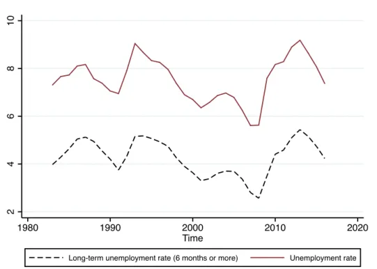
Figure 2 depicts the evolution of the unemployment rate ( ) and the long-term unemployment rate ( ) from the 1980s to recent times.Specifically, we refer to the average values of total and long-term unemployment rates with respect to 25 OECD countries between 1983 and 2016. Upon visual inspection, there is no sizeable increase in the : in 2016, it was still comparable to its initial level of 1983 (about 4.2% and 4%, respectively). More importantly, the has tracked down in relation to the in almost exactly the same way that it tracked up. In OECD countries, the peaked at 5.4% in 2013, not much higher than its value in 1994 when it peaked at 5.2%. Accordingly, the observation that ‘there is no sign
that the pool of supposedly less employable long-term unemployed people, which has so preoccupied economists and governments, ever existed’ (Webster, 2005, p. 978) seems to still be
valid in the last decade, which is characterized by a generalized increase in the unemployment rate.18
long-term unemployment and the total unemployment rate turns out to be a ‘normal relationship’, that is, a symmetric one (Webster, 2005, p. 985). In this respect, some exploratory evidence for OECD countries indicates that the relationship between the unemployment rate and its incidence is stronger and presents less dispersion when using the lagged rate of unemployment instead of the current (see Figures A2.1 and A2.2 in Appendix 2). Importantly, the issue of time lags has also been mentioned in Bean (1994), who labeled the attitude of empirical literature in analyzing the European (long-term) unemployment patterns as ‘cavalier’. Note that the long-term unemployment data comes from the OECD labor force statistics and are only available at the annual frequency: this may limit the identification of the appropriate time lag to be used.
16 By contrast, a variety of works have underlined that the progressive flexibilization of the labor market in mature
economies during the last three decades (Seccareccia, 1996; Stockhammer, 2011; Tridico, 2012, 2013; Brancaccio et al., 2018; Hein et al., 2020) substantially failed to favor employment recovery (Baccaro and Rei, 2007; Howell et al., 2007; Adascalitei and Morano, 2015; Brancaccio et al., 2020).
17 To further avoid cyclicality issues, in the empirical part of the paper we use also an additional definition of
long-term unemployment rate, as the ratio between and the working-age population.
18 This exercise is not intended to argue that long-term unemployed do not suffer from a worse condition than the
short-term unemployed. In this regard, Ochsen and Welsch (2011) documented an association between the duration of unemployment and its social costs. Our intent is simply to provide evidence against their lower employability, as advocated by a variety of contributions reported in Section 2.1, and to support the view that their status is not worsened in recent times.
Figure 2. Unemployment and long-term unemployment
The two lines identify the dynamics of the unemployment rate and the long-term unemployment rate (average values for 25 OECD countries). Correlation is 0.94 in levels and 0.78 in first differences.
In essence, this preliminary evidence suggests that when the overall unemployment rate falls, its long-term component also decreases. A closer look at the period between 1993 and 2008 indicates that the unemployment rate started its downswing one year before the : in 1993, the peaked at approximately 9%, while in 2008 it was 5.6% (the lowest value of the series). In parallel, the peaked one year after the peak of the and then tracked this latter almost perfectly (with a lowest value of 2.6% in 2008).
The synchrony of total and long-term unemployment rates is confirmed at the country level as well for almost all the countries included in our panel, as depicted in Figure A3.1 (reported in Appendix 3 for reasons of space).19
To further assess the relationship between the and the we also examine the dynamic patterns for the OECD aggregate and for some selected countries. Figure 3 plots the average trend for the 25 mature economies considered in this work. Remarkably, we can appreciate the existence of some loops from this two-axis representation. According to the NK explanation
19 Of course, some discrepancies among countries exist in terms of levels of both variables. Essentially, these may
depend on different macroeconomic trends, as well as on institutional and demographic patterns. While interesting and important for policy advice, this is, however, outside the scope of the present research, which is intended to provide general trends across mature economies.
2 4 6 8 10 1980 1990 2000 2010 2020 Time
of hysteresis, due to the structural feature of long-term unemployment, we should expect a clockwise movement between the two variables: when the falls, the should remain elevated. On the contrary, in Figure 3, by connecting consecutive dots (each one representing one year from 1983 to 2016), a counterclockwise movement emerges. The takeaway message of this scatter plot is therefore quite clear: when one variable increases, the other increases too (and vice versa).20 As a paramount example, between 1983 and 1987, the average
increased about 1 percent point (from approximately 7.3% to 8.2%), and the same happened with the (from approximately 4% to 5.1%). In the subsequent period, while the fell to 7% (in 1991), the collapsed to 3.7%. More recently, after the Great Crisis, the
started to increase (from 5.6% up to 9.2% in 2013). Meanwhile, the presented the same pattern, rising from 2.6% in 2008 to 5.4% in 2013. When the recovery partially occurred, we observe a downswing in the , along with a fall in the : in 2016, they settled at 7.4% and 4.2%, respectively.
Some country-specific cases confirm the general tendency for OECD economies: the cases of France, Germany, Italy, Spain, the United Kingdom and the United States are depicted in Figure A3.2 (Appendix 3). Quite interesting is what has happened in the post-Great Crisis period: the case of the United States is emblematic, where we observe a sharp increase in both variables from 2008 to 2009. In the subsequent years, the data may lead to the aforementioned ‘long-term unemployment trap’ (Webster, 2005). In fact, from 2009 to 2010, at the very beginning of recovery, while the unemployment rate was virtually unchanged (from 9.3% to 9.6%), the shows a sizeable increase (from 2.9% to 4.2%). When the recovery intensified, however, the two rates started to co-move again: from 2010 to 2016, the decreased by four percentage points, and similarly the decreased (from 4.2% to 1.2%). The sharp reabsorption of long-term unemployment observed in the United States is less evident in some European countries, such as Italy and Spain, due to the slower (or even null) recovery after the Great Recession and the ensuing persistence of high levels of unemployment, which produced an increasing stock of long-term unemployed people. Nevertheless, the direction of the relationship is generally confirmed, and this leads us to consider the macroeconomic outlook as likely to affect both the and the in a very similar way.
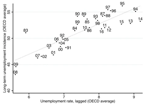
As we have seen that the tracks the dynamics of the with some lags, we also find it useful to linger on the possible relationship between past levels of the unemployment rate and current levels of the long-term unemployment rate. To this purpose, Figure 4 represents the relationship between the lagged and the current for the whole panel under scrutiny (pooled data). Intuitively, a positive correlation is confirmed at various levels of unemployment, and no signal of non-linearity is observed for higher unemployment rates. This appears to be inconsistent with the NK framework outlined above, as reabsorbing higher pools of long-term unemployed people is supposed to be even more problematic (Duell et al., 2016; Mathy, 2016). Nevertheless, evidence indicates that in correspondence with the lowest rates of total unemployment, the correlation between the and the lagged is less intense. The two different slopes drawn in the figure suggest that when unemployment is very low (below 4%,
20 The work by Webster (2005) suggests that even the use of the long-term unemployment incidence (instead of the
rate) would not produce the clockwise loops, testifying an inverse relationship between total and long-term unemployment, in case variables are considered with an appropriate delay.
which may be taken to represent frictional unemployment), people who have been without a job for long spells actually are, or are expected to be, more likely to have some individual characteristics that make them less employable. Put differently, this evidence suggests that when the labor market is tight, it becomes convenient for employers to use the individual unemployment spell as a signal of unobserved characteristics, as discussed in Section 2.1. Accordingly, the long-term unemployment stigma (Machin and Manning, 1999; Krug et al., 2019) seems to be at work mostly in the case of a tight labor market (Steffes and Biewev, 2008; Kroft et al., 2013; Shi et al., 2018).
Figure 4. Unemployment and long-term unemployment rates in OECD countries
The regression coefficient (pooled data, 25 countries, 1983–2017) is 0.42 for values of the unemployment rate lower than 4% (yellow line), while 0.80 for values of the unemployment rate higher than 4% (red line). Coefficients are 0.37 and 0.77 if we consider data as a panel.
All in all, evidence we have provided so far casts doubt on the validity of the NK thesis of the non-reversibility of long-term unemployment. On the contrary, our evidence suggests the existence of
symmetrical dynamics between the unemployment rate and its long-term component during both
phases of recession and recovery. This indicates that the evolution of both variables may be explained by the same factors (Rodriguez-Gil, 2018). Nor does our analysis support the view that there is more stickiness in the decrease in the long-term unemployment rate than in its increase. Finally, we find evidence confirming that the likelihood of firms screening workers on the basis of their unemployment spell is greater in the context of a tight labor market than in a slack one. While all these elements suggest that long-term unemployment should be considered a reversible phenomenon, we cannot yet assert that its fall would not generate accelerating inflation, as the NK
0 5 10 15 20 25 L o n g -t e rm u n e mp lo yme n t ra te 0 10 20 30
approach suggests. For this reason, the next section will focus on specific cases of long-term unemployment reductions and the subsequent inflation dynamics.
4. The non-inflationary effect of long-term unemployment reductions
In the previous section, we focused on the connection between the total and long-term unemployment rates. After having provided some descriptive evidence suggesting that the two indicators go hand in hand, we concluded that decreasing unemployment is generally associated with reductions in the . Nonetheless, an additional step is needed to assess the NK explanation of hysteresis: we are interested in verifying whether sizeable reductions in long-term unemployment are likely to generate significant inflationary pressures. If not, it will provide further support for the need to reconsider the NK hysteresis models introduced in Section 2. Thus, in this section, we undertake an econometric analysis that will try to deal with the following issue: what happens to the pace of inflation during and after a sizeable reduction in long-term unemployment? To the best of our knowledge, no empirical works have addressed this issue yet. For this reason, it represents a focus of and major challenge for our investigation.
4.1 Estimation strategy
4.1.1 Data and methodology
Before turning to the econometric estimations, let us describe the approach we will follow in our inquiry. To assess the effect of reductions in long-term unemployment on inflation, we make use of yearly data provided by the OECD and AMECO. According to data availability, we focus on 25 advanced economies for the period 1983–2016. A detailed list of countries in our sample can be found in Appendix 4. Notably, the selection of countries is also in line with the current literature on hysteresis, which principally involves mature economies (Ball, 2009, 2014; Blanchard et al., 2015; Girardi et al., 2020).
As explained in Section 3, we will focus on the long-term unemployment rate (and its dynamics), and we consider the long-term unemployed as individuals who have been looking for work for at least six months. We first calculate the as defined in Equation (6). Subsequently, for each country ( ), we calculate the annual percentage change in the . Significantly, we do not use its first differences, and we do so in order to take into account the intensity of the variation: the intuition behind this choice is that a one-point reduction in the level of the may have different impacts on macroeconomic outcomes, such as inflation, depending on whether it occurs when a relatively high or low level of the prevails. For this reason, we prefer to use the percentage rate of change in the long-term unemployment rate, as in Equation (7):
(7).
As a second step, we introduce an identification strategy to define episodes of ‘sharp’ or ‘sustained’ reductions in the long-term unemployment rate. The rationale behind this approach is to assess the effect on inflation of sharp decreases in the compared to cases where such a
circumstance did not occur. Our findings will therefore represent the magnitude of inflationary surges experienced by ‘treated’ units (country-years with a strong decrease in the ) with respect to ‘control’ units (country-years without such a decrease).
To detect strong reductions in long-term unemployment, we focus on negative values of the exclusively, and we calculate the country average ( ) as well as the standard deviation ( ). Therefore, we identify an reduction as a strong one when the observation for country at time satisfies the following criteria (C1 and C2):
(C1) with
<0 (C2).
Consistent with our approach, these selected episodes represent our treatment group, while observations not satisfying these criteria will belong to the control group. To directly identify the observations according to our yardstick, we built a dummy variable ( ) which assumes the value of 1 during an episode of sustained long-term unemployment reduction (that is, in case of a shock) and 0 otherwise. This ‘average treatment effect’ methodology is at the core of our investigation and offers valuable insights into our research question: we are interested in assessing whether sharp episodes of reductions (the treated group) are, on average, associated with higher inflation than country-years in which this sharp reduction does not occur (the control group), after controlling for country and time fixed effects.
In our sample, we detect 430 country-year observations featuring a decreasing long-term unemployment rate (that is, by ). By following our identification strategy, we isolate 78 cases of sharp long-term unemployment reduction and 721 non-episodes. Importantly, the control group is composed of both observations characterized by an increase in the
(369) and observations that present a ‘moderate’ reduction (352). In Appendix 4, we indicate how episodes of long-term unemployment reductions are distributed among countries, while in Appendix 5, the complete list of episodes is reported.
4.1.2 Size of the treatment
As a second step, we aim at assessing whether the sample of treatedis adequately representative of the treatment received, that is, if the selected episodes can effectively identify sizeable reductions in the compared with the control group. To prove this, we use alternative empirical techniques. At first, by employing a standard t-statistics test, we aim at verifying whether the difference between the average values of considered variables are statistically significant
between the two groups. Furthermore, to validate the representativeness of the treated sample, we also employ linear regression techniques by estimating the following Equation (8):
(8) where the dependent variable is the rate of change of the long-term unemployment rate; is the dummy variable of identified episodes; represents country-specific fixed-effects; identifies year dummies; and is the error term. When the coefficient is found to be significant, a statistically significant difference between treated and control groups exists.
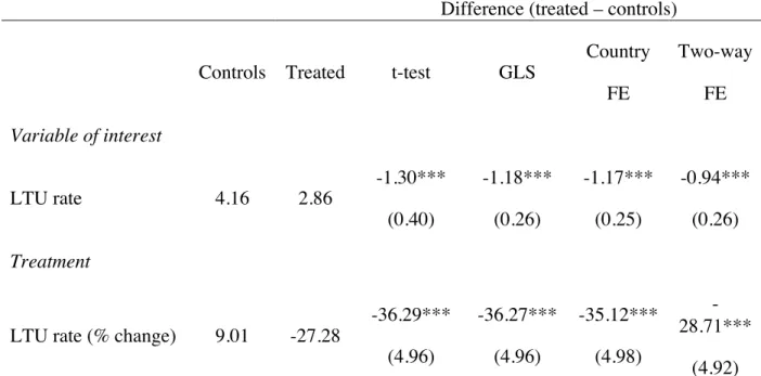
Table 1 presents the results of tests on the size of the treatment. The average percentage change in the long-term unemployment rate ( ) settles at +9% in the control group, while it is -27% in the treated one. When implementing a mean comparison, the difference between treated and controls is highly statistically significant. Differences are confirmed in all specifications when we extend the analysis to regression-based techniques. In particular, we first estimate the relation without controls (‘GLS’ column); second, we estimate a fixed-effects model that only controls for country-specific effects (‘Country FE’); and finally, we run a two-way fixed-effects model that controls for a full set of country and year effects (‘Two-way FE’). The differences between the average values of the two samples are statistically significant in all specifications, and it is approximately equal to 30%.21 These findings confirm that the selected episodes are reliable and
refer to sharp reductions in the long-term unemployment rate. We also provide evidence (see below) that the changes in long-term unemployment in the ‘treated’ determine a difference with respect to the control group that is not temporary, but lasts over the chosen five years window.
21 For the sake of verifying whether such episodes occur independently (or not) on the magnitude of the long-term
unemployment rate, we replicate the same analysis on the taken in levels. Results (reported in Table 1)
indicate that the level of the long-term unemployment rate is 4.16% in the control group while it is 2.86% in the treated
Table 1. Size of the treatment
Difference (treated – controls)
Controls Treated t-test GLS
Country FE Two-way FE Variable of interest LTU rate 4.16 2.86 -1.30*** (0.40) -1.18*** (0.26) -1.17*** (0.25) -0.94*** (0.26) Treatment
LTU rate (% change) 9.01 -27.28
-36.29*** (4.96) -36.27*** (4.96) -35.12*** (4.98) -28.71*** (4.92)
The table reports the average decrease in long-term unemployment during episodes of reductions (relative to non-expansion observations). Coefficients are multiplied by 100 for ease of interpretation (so a coefficient of 1 means a 1% difference). We employ a linear regression to compare the mean of the variable in the year of a ‘strong’ reduction of the long-term unemployment rate with the mean in the rest of the sample. The test is applied using three models: a GLS which considers the panel structure of data (‘GLS’); a fixed-effects model that only controls for country-specific effects (‘Country FE’); and a two-way fixed-effects model which controls for a full set of country and year effects (‘Two-way FE’). Robust standard errors clustered by country in parentheses; *** p<0.01, ** p<0.05, * p<0.1.
4.1.3 Endogeneity issues
A problem, however, might undermine our identification strategy: episodes of long-term unemployment reduction (that is, our shocks) may present a certain degree of endogeneity perhaps caused by changes in variables that also have an impact on (or reflect changes in) our dependent variable, that is, the inflation rate. For example, the long-term unemployment rate may be supposed to decrease in connection with sizeable surges in output, an element that may – other things being equal – stimulate the pace of inflation because of bottlenecks in capacity (fixed capital) rather than in the labor market. Alternatively, inflationary surges (or reductions) may be affected by the dynamics of the real effective exchange rate (or productivity), which in turn could produce effects on the levels of output and unemployment as well. In addition, movements in the policy interest rate might influence unemployment and at the same time result from pre-existing price dynamics, since in setting it, the monetary authority usually takes into account the pace of inflation (as discussed in Section 2.2).
particular, we verify whether shocks are likely to be randomly assigned. In doing so, we focus on what happened the year before each treatment, and particularly, we verify whether relevant discrepancies between treated and non-treated observations hold with respect to a range of macroeconomic indicators. Put another way, we look at potential differences in economic preconditions in order to establish whether our shocks can be considered sufficiently exogenous for the purpose of studying the evolution of the inflation rate during and after the shocks. To do so, similar to what has been done in Equation (8), we apply a linear regression by considering each macroeconomic variable in the year before the shock ( ) as our endogenous variable, and as our exogenous variable the dummy variable including the shocks. We are interested in the coefficient , whose statistical significance would indicate differences between the average values of each selected macroeconomic indicator between episodes and non-episodes in the year preceding the shock. Formally, we estimate the following regression (Equation 9):
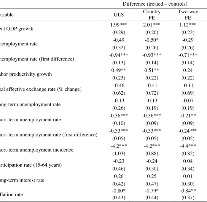
(9) where represents the macroeconomic variable of interest; is the dummy variable already introduced; and are country and year fixed effects, respectively. Table 2 reports the results of the linear regressions undertaken to compare the mean of each variable in the year before the shock with the mean in the rest of the sample. The first column refers to a GLS regression in which we do not control for country and year fixed effects (thus assuming = for all countries and = 0 for all years). Then, in the second column, we allow for country (but not year) fixed effects ( = 0 is still assumed for all t). Finally, in the third column, we include a full set of country and year fixed effects. Importantly, in our framework, this latter test represents the strongest way to control for potential endogeneity since it allows for the comparison of treated and non-treated countries within each year. After controlling for country-time fixed effects, endogeneity virtually disappears for a number of macroeconomic preconditions. Nevertheless, some discrepancies between treated and controls remain with respect to some variables. Specifically, coefficients on GDP growth, on the change in the unemployment rate and on short-term unemployment (both the rate and its incidence) are significant. Finally, we also detect a statistically significant difference for what concerns the inflation rate, our variable of interest, which turns out to be somewhat higher (0.8%) in the control group than in the treated, an element which suggests the need to control for the pre-existing trend in inflation in our estimations.
Table 2. Comparison of lagged macroeconomic conditions in treated and non-treated observations
Difference (treated – controls)
Variable GLS Country FE Two-way FE Real GDP growth 1.99*** 2.01*** 1.12*** (0.29) (0.20) (0.23) Unemployment rate -0.49 -0.50* -0.29 (0.32) (0.26) (0.26)
Unemployment rate (first difference) -0.94*** -0.93*** -0.71***
(0.13) (0.14) (0.14)
Labor productivity growth 0.49** 0.51** 0.24
(0.23) (0.22) (0.22)
Real effective exchange rate (% change) -0.46 -0.41 -0.11
(0.62) (0.72) (0.69)
Long-term unemployment rate -0.13 -0.13 -0.07
(0.26) (0.19) (0.19)
Short-term unemployment rate -0.36*** -0.36*** -0.21**
(0.10) (0.09) (0.09)
Short-term unemployment rate (first difference) -0.33*** -0.33*** -0.24***
(0.05) (0.05) (0.05)
Short-term unemployment incidence -4.2*** -4.2*** -4.4***
(1.03) (0.88) (0.82)
Participation rate (15-64 years) -0.23 -0.24 0.04
(0.46) (0.50) (0.34)
Long-term interest rate 0.26 0.25 0.01
(0.42) (0.47) (0.30)
Inflation rate -0.80* -0.79* -0.84**
(0.43) (0.44) (0.37)
For each variable, we employ a linear regression to compare the mean of the variable in the year before a ‘sustained’ long-term unemployment reduction with the mean in the rest of the sample (Equation 9). Coefficients are multiplied by 100 for ease of interpretation. The test is applied using three models: a GLS which considers the panel structure of data (‘GLS’); a fixed-effects model that only controls for country-specific effects (‘Country FE’); and a two-way fixed-effects model which controls for a full set of country and year effects (‘Two-way FE’). Robust standard errors clustered by country in parentheses; *** p<0.01, ** p<0.05, * p<0.1.
The statistical significance of some macroeconomic preconditions merits explicit discussion. Unsurprisingly, estimates indicate that lagged GDP growth is associated with long-term unemployment reductions. Moreover, the coefficient of the lagged change in the unemployment rate is negative: this could be interpreted as an additional signal of a quasilinear association between the dynamic of total and long-term unemployment, as discussed in Section 3. In other words, this precondition further testifies that episodes of strong long-term unemployment reduction are likely to happen in the context of decreasing unemployment rates. We also find a negative and significant coefficient associated with short-term unemployment: this indicates that episodes of sustained decreases in the
are associated, on average, with lower short-term unemployment as well. Yet, this precondition would produce even more acceleration in the pace of inflation, according to the NK theory of hysteresis (Llaudes, 2005). For this reason, this initial condition would eventually strengthen our result if we do not find any signal of inflationary pressures during and after our shocks.
All in all, preconditions indicate that our episodes tend to occur, on average, in a macroeconomic context that is more likely to generate inflation, that is, one featuring growing income, decreasing unemployment and lower short-term unemployment. Therefore, if no signal of inflation surges is detected, our analysis will be reinforced by these contextual conditions. However, to overcome as much as possible endogeneity issues in our estimations, we will explicitly control for all the macroeconomic preconditions that turned out to be significantly different in our episodes of strong long-term unemployment reduction vis à vis the control group: practically, we will insert these (lagged) variables as additional regressors, with a view to controlling for the pre-treatment trends of these variables (cf. Girardi et al., 2020). Furthermore, it has to be recalled that in all our estimates we will make use of time- (in addition to country-) fixed effects: being our dependent variable taken in annual changes, this strategy will further mitigate the endogeneity bias, if any, inasmuch year dummies would capture the presence of potential omitted variables which would simultaneously affect both inflation and LTU shocks.
4.1.4 Model specification
Having identified episodes of strong reductions in the , and after having dealt with potential endogeneity challenges, we now turn to the model specification. Of particular interest for the sake of our purposes is the approach suggested by Jordà (2005) and recently reappraised by a variety of works (see, among them, Teulings and Zubanov, 2014; Girardi et al., 2020). This method is commonly termed local projections (henceforth, LPs). In particular, it allows us to assess the average treatment effect of strong decreases in long-term unemployment on inflation. As we are wishing to evaluate the effect of our shocks on inflation at different time horizons, LPs are particularly appealing. Specifically, through this scheme, we will estimate the average behavior of inflation in the five-year period which follows the shocks by means of impulse response functions (henceforth, IRFs) and compare it to what happens in non-episode observations. Formally, the dynamic model we estimate is represented by the following Equation (10):
(10)
• is the inflation rate at different points in time (from to , with identifying the year when the shock occurs);
• is the inflation rate in the year before each shock;
• is the dummy variable identifying shocks (and assuming the value of 1 in the case of a shock);
• is the vector of control variables, jointly or alternatively considered, that turned out to be relevant as initial conditions;
• and identify country and year fixed effects, respectively; and • denotes the error term.
As suggested in Section 4.1.3, a two-way fixed-effect specification is preferable since it avoids endogeneity with respect to many preconditions. Moreover, this specification helps us in taking into account the heterogeneity among countries and in comparing the response to our shocks in different countries within each year. Finally, since our sample is composed of different economies that are considered for a relatively long time span, this approach presents a number of advantages with respect to a standard VAR-based model: our strategy for the estimation of IRFs is more flexible than a VAR as LPs allow a semi-parametric estimation of the ‘average treatment effect’ of long-term unemployment reductions at different time horizons, without assuming any underlying parametric model for the outcome variable (Girardi et al., 2020). As this approach imposes little structure on the data, it turns out to be particularly appealing in our setting. On the contrary, with a VAR or dynamic panel estimations, we would impose a single parametric model: for this reason, these models would be extremely sensitive to mis-specification of the data-generating process, and this sensitivity becomes more important as the time horizon increases. Notably, LPs are instead robust to mis-specification of the data-generating process and thus have been recently used for the assessment of medium-run effects of negative macroeconomic shocks (Teulings and Zubanov, 2014).
According to our estimation plan, when presenting and discussing our findings (Sections 4.2 and 4.3), we will focus on the size and significance of : indeed, this coefficient represents the effect at the year of an episode of sharp long-term unemployment reduction occurring in the year , a coefficient which will be plotted by means of our IRFs. Through the assessment of this coefficient, we aim at evaluating the average effect of a negative shock in the at different time horizons, relative to the control group of observations.
4.2 Findings
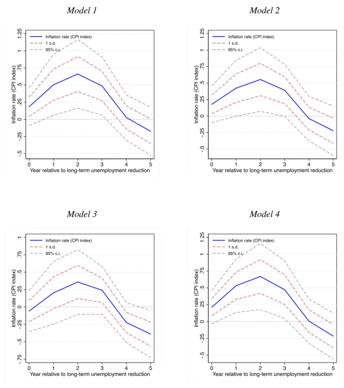
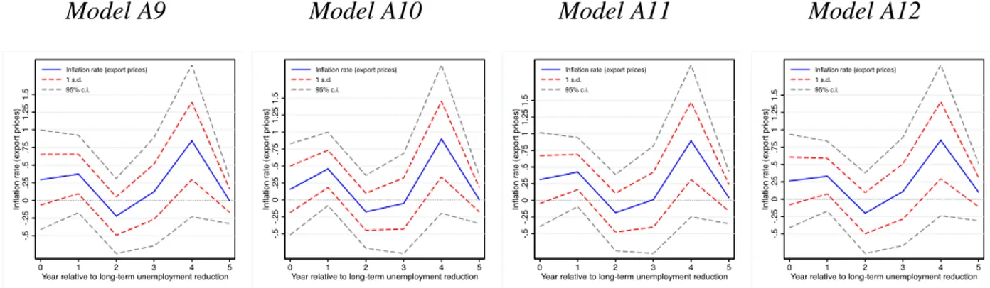
In our baseline estimations, we will focus on the effect of sharp long-term unemployment reduction on the inflation rate measured as the annual percentage change in the consumer price index (CPI). Importantly, in all our estimations, we do control for the pre-existing trend in inflation (that is, by including the lagged inflation rate in all specifications) because it is standard in the framework of LPs (Jordà, 2005). Our findings are depicted in Figure 5 and reported in Table 3. Model 1 is the baseline model to which we do not add additional controls, while in Models 2 to 5, we include as
controls the variables that have been found to potentially cause a selection bias. Specifically: in Model 2, we control for the lagged change in the short-term unemployment rate; in Model 3, we include the lagged variation of the unemployment rate; in Model 4, we control for the lagged incidence of short-term unemployment; and finally, Model 5 simultaneously includes the two control variables considered in Models 3 and 4.
As far as the very baseline model is concerned, findings indicate that sustained decreases in long-term unemployment have very moderate effects on CPI-inflation: while at the onset the effect is virtually null, it becomes positive and statistically significant (at the 95% level) one year after the shock, although it is very low in size. On average, in treated observations, the inflationary pressure peaks two years after the shock (0.66 percentage points more than the control group) and then starts decreasing, to the point that it becomes null at time , pictured as an ‘inverted-U’. This pattern indicates that there is no trace of accelerating or even persistent inflation phenomena as the NK approach would predict after a severe reduction in the long-term component of unemployment.
Figure 5. Effect of a long-term unemployment reduction on inflation rate Model 1 Model 2 Model 3 Model 4 -. 5 -. 2 5 0 .25 .5 .75 1 1.25 In fla tio n ra te (C PI in d e x) 0 1 2 3 4 5
Year relative to long-term unemployment reduction
Inflation rate (CPI index) 1 s.d. 95% c.i. -. 5 -. 2 5 0 .25 .5 .75 1 1.25 In fla tio n ra te (C PI in d e x) 0 1 2 3 4 5
Year relative to long-term unemployment reduction
Inflation rate (CPI index) 1 s.d. 95% c.i. -. 7 5 -. 5 -. 2 5 0 .25 .5 .75 1 In fla ti o n ra te (C PI in d e x) 0 1 2 3 4 5
Year relative to long-term unemployment reduction
Inflation rate (CPI index) 1 s.d. 95% c.i. -. 5 -. 2 5 0 .25 .5 .75 1 1.25 In fla ti o n ra te (C PI in d e x) 0 1 2 3 4 5
Year relative to long-term unemployment reduction
Inflation rate (CPI index) 1 s.d.
Model 5
The graphs display the IRFs of a strong reduction in the long-term unemployment rate on the inflation rate. They are obtained through local projections, controlling for a full set of country and year fixed effects and one lag of the inflation rate. In Model 1 we do not include additional controls. In Model 2 we control for the lagged change of short-term unemployment rate. In Model 3 we include the lagged variation of the unemployment rate. In Model 4 we control for the lagged incidence of short-term unemployment. Model 5 combines Models 3 and 4. Years relative to the LTU reduction on the horizontal axis. Coefficients are reported in Table 3. Percentage points on the vertical axis. Robust standard errors clustered by country.
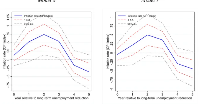
When adding some control variables, inflation surges almost totally disappear. In detail, when we control for the lagged change in unemployment rate (Models 3 and 5), no statistically significant discrepancies in terms of inflation are detected between the treated and the control group: contrary to what is postulated by the NK explanation of hysteresis, we find lower inflation instead in treated units than in the control group 5 years after the shock. Models 2 and 4 also incorporate lagged short-term unemployment, considered in terms of both its rate and incidence, respectively. In addition, in these cases, the response of inflation is null on impact. Inflation surges become moderately positive and statistically significant from to (peaking in at 0.55 and 0.67 in the two models, respectively), but they return to 0 when the time window approaches
-. 7 5 -. 5 -. 2 5 0 .25 .5 .75 1 In fla tio n ra te (C PI in d e x) 0 1 2 3 4 5
Year relative to long-term unemployment reduction
Inflation rate (CPI index) 1 s.d.
Table 3. Dynamic effect of a long-term unemployment reduction on CPI-based inflation rate
Year 0 Year 1 Year 2 Year 3 Year 4 Year 5
Model 1 0.18 0.50** 0.66** 0.49** 0.03 -0.17 (0.14) (0.23) (0.26) (0.22) (0.17) (0.18) Model 2 0.18 0.42* 0.55** 0.39* -0.04 -0.22 (0.14) (0.22) (0.25) (0.20) (0.17) (0.19) Model 3 -0.06 0.20 0.36 0.24 -0.22 -0.39** (0.15) (0.23) (0.24) (0.18) (0.15) (0.17) Model 4 0.21 0.53** 0.67** 0.47** 0.01 -0.22 (0.13) (0.20) (0.25) (0.22) (0.17) (0.17) Model 5 -0.01 0.26 0.38 0.23 -0.25 -0.41** (0.13) (0.21) (0.24) (0.18) (0.15) (0.17) Observations 799 774 749 724 699 674 Episodes 78 74 72 69 69 69
Effects estimated through local projections (see Equation 10). Coefficients are multiplied by 100 for ease of interpretation (so a coefficient of 1 means a 1% increase in the variable). All regressions control for a full set of country and year fixed effects and for one (pre-treatment) lag of the dependent variable. Robust standard errors clustered by country in parentheses; *** p<0.01, ** p<0.05, * p<0.1.
Our results are validated by the fact that the identified shocks produce persistent effects on long-term unemployment itself. As it can be seen in Appendix 6, in year the in the treated group is approximately 1 percent point below the control group, and subsequently it remains at lower level; at we witness a negative peak in this gap (about -1.2 p.p., statistically significant at the 95% level). This clarifies that episodes constitute, on average, persistent decreases in the relative to the control group. Moreover, it confirms that the non-inflationary effects of sharp reductions in long-term unemployment do not depend on a sudden reabsorption of the shock. All in all, evidence we provide does not confirm the existence of a sizeable inflationary risk associated with a sustained decrease in long-term unemployment, even when we control for initial macroeconomic conditions. Our findings are therefore at first glance in stark contrast to the NK narration of hysteresis based on the role of the long-term unemployed. Our episodes of sharp reductions in the long-term unemployment rate turned out to be associated with very small, short-lived and in most cases statistically insignificant effects on inflation, with no sign of acceleration: