A
A
l
l
m
m
a
a
M
M
a
a
t
t
e
e
r
r
S
S
t
t
u
u
d
d
i
i
o
o
r
r
u
u
m
m
–
–
U
U
n
n
i
i
v
v
e
e
r
r
s
s
i
i
t
t
à
à
d
d
i
i
B
B
o
o
l
l
o
o
g
g
n
n
a
a
1 2DOTTORATO DI RICERCA IN
3 4Scienze e Tecnologie Agrarie, Ambientali e Alimentari
56
Ciclo XXX
7 8
Settore Concorsuale: 07/B2 – SCIENZE E TECNOLOGIE DEI SISTEMI ARBOREI E FORESTALI
9
Settore Scientifico Disciplinare: ASSESTAMENTO FORESTALE E SELVICOLTURA
10 11
TITOLO TESI
12 13
Disentangling the effects of age and global change on Pseudotsuga menziesii (Mirb.) Franco growth and 14
water use efficiency 15
16 17
Presentata da:
Dott. Dario Ravaioli
1819 20
Coordinatore Dottorato
Supervisore
21
Prof. Giovanni Dinelli
Prof. Federico Magnani
22
Co-Supervisore
23Dott. Fabrizio Ferretti
24 25 26 27
Esame finale anno 2018 28
Abstract
30The recent alterations in forests growth could be the result of a combination of different climatic 31
and non-climatic factors, as rising atmospheric [CO2], temperature fluctuations, atmospheric
32
nitrogen deposition and drought stress. This study tests the potential effects of global change on 33
trees, assessing the relative importance and functional relationships between environmental drivers 34
and long-term growth trend, as well as physiological response. To investigate such effects, we 35
applied Generalized additive models (GAMs) technique, decoupling the non-linear age related 36
effect from co-occurring environmental effects on basal area increments (BAI) series and isotope 37
proxies (δ13C and δ18O). Two Douglas fir (Pseudotsuga menziesii (Mirb.) Franco) chronosequence 38
were considered; the first one, comprises four different age classes (age 65-, 80-, 95- and 120-) and 39
is a even-aged stands plantation located in Italy, while the second one is an old-growth Californian 40
stand, with three age classes (age 100, 200, 300). Results show a 22.9% decrease of the general BAI 41
growth trend over last decades for the Italian Douglas-fir chronosequence, when the age-size non-42
linear effect was removed. A related trend in water use efficiency (iWUE=Amax/gs,the ratio between
43
photosynthetic assimilation and stomatal conductance) was observed in the same period. Thus, 44
through the application of the so called dual isotope approach, was possible to attribute to a 45
reduction in Amax the cause of such a trend, probably driven by a reduction in N deposition. On
46
other hand, BAI trend accounted for the Californian old-growth stand shows an increase of roughly 47
the 60% since the 1960, which was found to be mostly determinate by a strong effect of 48
atmospheric [CO2]. These founding highlight how this species has been affected by global change
49
impact in both sits and provide important insights on its future behavior, potentially driving 50
management choices. 51
Key words: Pseudotsuga menziesii, BAI, iWUE, long-term trends, global change, GAMs, isotope 52
dual approach. 53
Summary
55
Abstract 56
Chapter I - Disentangling the effects of age and global change on Douglas-fir growth... 9 57
1. Introduction... 9 58
2 Materials and methods... 11 59 2.1 Study area... 11 60 2.2 Tree-ring data ... 13 61 2.3 Environmental data ... 14 62 2.4 Data analysis... 17 63 3 Results ... 19 64 3.1 Dendrochronology... 19 65 3.2 Model output... 22 66 4. Discussion ... 26 67 5 Conclusions... 27 68 6. Acknowledgments ... 28 69 7. Bibliography... 29 70
Chapter II - Douglas fir eco-phisiological response to global change... 36 71
1. Introduction... 36 72
2. Material and Methods... 38 73
2.1 Study area... 38 74
2.2 Samples preparation and isotopic analysis ... 40 75
2.3 δ13C theory... 41 76
2.4 δ18O theory ... 43 77
2.5 Dual isotope conceptual model... 45 78
2.6 GAM model... 46 79
3. Results ... 48 80
3.1 Effects of cellulose extraction... 48 81
3.2 Carbon isotope and iWUE dynamics ... 49 82
3.3 Oxygen isotope dynamics... 56 83
3.4 Dual isotope approach... 61 84
4. Discussion ... 62 85
4.1 Age-related effects ... 62 86
4.2.Environmental and biogeochemical effects... 63 87
5.Conclusions... 67 88
6.Bibliography... 68 89
Chapter III - Old-growth stand trees reaction to global change, an explorative study... 75 90
1. Introduction... 75 91
2 Material and methods... 78 92 2.1 Study area... 78 93 2.2 Sampling strategy ... 79 94 2.3 Tree-ring data ... 81 95 2.4 Climate data... 83 96 2.2 Geochemical data... 85 97 2.3 GAMs ... 86 98
3. Results and discussion... 87 99 4. Conclusions... 95 100 5. Bibliography... 97 101 102 103
General introduction
104105
The ongoing global changes are intimately linked to the increase in the concentration of greenhouse 106
gases in the atmosphere, due to anthropogenic emission. The lower degree of infrared solar 107
radiation that can be dissipated out of the earth system results in an increase in global average 108
temperatures, attended to reach levels included between 2°C up to 4.5°C degrees by the end of this 109
century, as well as an alteration of extent and distribution of precipitation (IPCC 2014). The main 110
greenhouse gas, CO2, has reached today a concentration of 406 μmol mol-1, the highest in the last
111
650000 years. Over the past 250 years, atmospheric CO2has been increased globally by the 30%
112
from the concentration of 285 ppm in the pre-industrial era, with an exponential progression. The 113
human carbon source, resulting by fossil fuel combustion and land use change, is estimated in 8.8 114
Gt C y-1. The main sinks, which absorb actively carbon from atmosphere, are oceans and terrestrial 115
ecosystems, able to remove roughly 2 Gt C each one every year. The extent of the terrestrial sink, 116
manly represented by forest ecosystems, is directly and indirectly influenced by global change. The 117
temperature variations can increase (enlarging the vegetative period)(Menzel and Fabian, 1999) or 118
decrease (water stress due to excessive evapo-transpiration)(Allen et al. 2010) plants' 119
photosynthetic assimilation. On the other hand, the greater amount of CO2 available to plants
120
photosynthesis could acts positively on the growth capacity of trees, amplifying their mitigating 121
effect (Ainsworth and Long 2005). For what concern the northern hemisphere and temperate forests 122
in particular was observed, both through satellite direct measurement of NDVI (Normalized 123
Difference Vegetation Index) and ground-based data, an increase in net primary productivity (NPP, 124
gross primary productivity minus autotrophic respiration, GPP-Ra) of 20% in the last decades of
125
the 20th century (Boisvenue and Running 2006). The causes were attributed for a 50% to direct 126
effects of forest management, for 33% to the direct and indirect effects caused by global change and 127
for 8-17% to historical effects related to age stands dynamics (Vetter et al. 2005). Contrarily, more 128
recent observations seem to highlight an inversion of this trend. The NPP in the first decade of the 129
new millennium suffers a global decrease, probably due to the drought events induced by higher 130
temperatures (Zhao & Running, 2010). A better understanding of how [CO2] acts on forests both
131
directly and through the improvement of positive or negative feedbacks, as which one involved 132
temperature and water stress process or trees growth enhancement, is of crucial importance. Indeed, 133
it determine the capacity of realize predictive reliable models on the future global change entity. 134
Another key factor determining these anomaly in forest growth has been identified in the potential 135
fertilizing effect of atmospheric nitrogen depositions (Hyvönen et al., 2007), caused by atmospheric 136
pollution of nitrogen oxidized (NOyderiving from combustion) and of reduced form (NHx deriving
137
from agricultural fertilization). Discounted the age-related effect, a quasi-linear relationship 138
between N depositions and net ecosystem productivity (NEP, difference between gross primary 139
productivity and total ecosystem respiration, GPP-R) has been hypothesized (Magnani et al. 2007), 140
caused by the direct nitrogen canopy uptake which can bypass bacterial competition in the soil and 141
the relative increase in heterotrophic respiration (Rh ,source of C). It would increase C sequestered
142
by plants in temperate forest ecosystems (typically N-limited) increasing their sink effect. 143
Furthermore, when long-term analysis on trees growth is performed, it should be taken into 144
consideration also that forests normally display a progressive reduction in productivity as stand age 145
increase. For example, Aboveground Productivity (Pa, one of the components of NPP) is influenced
146
by age-size related dynamics in the leaf area index (LAI, defined as the relationship between the 147
photosynthetically active leaf surface and the surface of the soil on which the leaves are projected). 148
After a juvenile phase of expansion, determining an increase in time of Pa, LAI reaches a
149
culmination at stand canopy closure, exceeded which the increase in inter-tree competition for 150
light, water and nutrients progressively reduces Pa (Ryan and Yoder, 1997). Another component of
151
this age-effect is explained by the hydraulic limitation hypothesis (HLH) which relates productivity 152
decrease and tree dimension. The gradual increase in hydraulic resistance with the increase of the 153
height of the stem, the length of the branches and the thickness of the roots, would cause an 154
enhancement in the internal water potential difference between roots and shoots, if hydraulic leaf 155
conductance (k) is maintained constant. Instead, a k reduction is observed with trees ageing, caused 156
by a decrease of stomatal conductance (gs). This link between hydraulic resistances and the degree
157
of stomatal closure affect net photosynthesis rates, decreasing the amount of CO2 which could be
158
assimilated in relation to LAI (Gower et a. 1996) .The maintenance of a almost constant leaf 159
potential, obtained through the reduction of stomatal conductance is a compromise between the 160
photosynthesis, water transport at greater heights (which would be more effective at more negative 161
leaf water potential) and cavitations avoidance (embolisms caused by the vascular system water 162
chain brake) which would be suffered by the xylem if extremely negative water potentials would be 163
reached (Tyree and Sperry, 1988; Magnani et al. 2000). 164
Separate these age-size related effects from the co-occurring environmental changes effects 165
affecting trees growth, is virtually impossible if a single age-class is considered because both of 166
them are time correlated (Bowmanet al., 2013). Indeed, exogenous effects, as climate-related 167
covariates or biogeochemical pollutants impact, varying along calendar year while age-size effects 168
(endogenous), varying along cambial age. To overcome such inter-correlation issues is possible to 169
apply a sampling strategy aimed on the collection of a wide range of age-classes from a multi-age 170
stand or from different even-aged stands growing in comparable environmental condition, but 171
established in different dates. This chronosequence-based approach sensu Walker et al. (2010) 172
allow to assess the effects of changing environmental conditions affecting tree growth (i.e, rising 173
[CO2], temperature or water availability) trough the deviation from the attended age-related mean
174
trend . Based on this eco-physiological and environmental background , the first objective of this 175
PhD thesis is to evaluate the possible impact of global change affecting two Douglas fir 176
(Pseudotsuga menziesii (Mirb.) Franco) chronosequences, separating age -related growth changes 177
from environmentally-driven long-term growth trends superimposed on them. The second aim is to 178
test the possibility to disentangling among singular environmental factors which one have mostly 179
determined long-term growth and eco-physiological response trend variations, with the idea of 180
highlight potential vulnerability or strength points exhibited by this species, also in a future 181
adaptation prospective of this species to the Italian environment. 182
183
Bibliography 184
Ainsworth, Elizabeth A., and Stephen P. Long. 2005. “What Have We Learned from 15 Years of Free-Air CO2 185
Enrichment (FACE)? A Meta-Analytic Review of the Responses of Photosynthesis, Canopy Properties 186
and Plant Production to Rising CO2.” New Phytologist 165 (2): 351–71. doi:10.1111/j.1469-187
8137.2004.01224.x. 188
Allen, Craig D., Alison K. Macalady, Haroun Chenchouni, Dominique Bachelet, Nate Mcdowell, Michel 189
Vennetier, Thomas Kitzberger, et al. 2010. “A Global Overview of Drought and Heat-Induced Tree 190
Mortality Reveals Emerging Climate Change Risks for Forests.” Forest Ecology and Management 259 191
(4): 660–84. doi:10.1016/j.foreco.2009.09.001. 192
Bowman, David M.J.S., Roel J.W. Brienen, Emanuel Gloor, Oliver L. Phillips, and Lynda D. Prior. 2013. 193
“Detecting Trends in Tree Growth: Not so Simple.” Trends in Plant Science 18 (1). Elsevier Ltd: 11–17. 194
doi:10.1016/j.tplants.2012.08.005. 195
Gower ST, McMurtrie RE, Murty D (1996) Aboveground net primary production decline with stand age: 196
potential causes. Trends Ecol Evol Res 11: 378-382. 197
Hyvönen, Riitta, Göran I Agren, Sune Linder, Tryggve Persson, M Francesca Cotrufo, Alf Ekblad, Michael 198
Freeman, et al. 2007. “The Likely Impact of Elevated [CO2], Nitrogen Deposition, Increased 199
Temperature and Management on Carbon Sequestration in Temperate and Boreal Forest Ecosystems: 200
A Literature Review.” The New Phytologist 173 (3): 463–80. doi:10.1111/j.1469-8137.2007.01967.x. 201
IPCC. 2014. Summary for Policymakers. Climate Change 2014: Synthesis Report. Contribution of Working 202
Groups I, II and III to the Fifth Assessment Report of the Intergovernmental Panel on Climate Change. 203
doi:10.1017/CBO9781107415324. 204
Magnani, F., M. Mencuccini, and J. Grace. 2000. “Age-Related Decline in Stand Productivity: The Role of 205
Structural Acclimation under Hydraulic Constraints.” Plant, Cell and Environment 23 (3): 251–63. 206
doi:10.1046/j.1365-3040.2000.00537.x. 207
Magnani, Federico, Maurizio Mencuccini, Marco Borghetti, Paul Berbigier, Frank Berninger, Sylvain Delzon, 208
Achim Grelle, et al. 2007. “The Human Footprint in the Carbon Cycle of Temperate and Boreal 209
Forests.” Nature 447 (7146): 848–50. doi:10.1038/nature05847. 210
Menzel, Annette, and Peter Fabian. 1999. “Growing Season Extended in Europe.” Nature 397 (6721): 659– 211
659. doi:10.1038/17709. 212
Ryan, Michael G., and Barbara J. Yoder. 1997. “Hydraulic Limits to Tree Height and Tree Growth.” 213
BioScience 47 (4): 235–42. doi:10.2307/1313077. 214
Tyree, M T, and J S Sperry. 1988. “Do Woody-Plants Operate Near the Point of Catastrophic Xylem 215
Dysfunction Caused By Dynamic Water-Stress - Answers From A Model.” Plant Physiology 88 (3): 574– 216
80. doi:10.1104/pp.88.3.574. 217
Vetter, Mona, Christian Wirth, Hannes Böttcher, Galina Churkina, Ernst Detlef Schulze, Thomas Wutzler, 218
and Georg Weber. 2005. “Partitioning Direct and Indirect Human-Induced Effects on Carbon 219
Sequestration of Managed Coniferous Forests Using Model Simulations and Forest Inventories.” 220
Global Change Biology 11 (5): 810–27. doi:10.1111/j.1365-2486.2005.00932.x. 221
Walker, Lawrence R., David a. Wardle, Richard D. Bardgett, and Bruce D. Clarkson. 2010. “The Use of 222
Chronosequences in Studies of Ecological Succession and Soil Development.” Journal of Ecology 98 (4): 223
725–36. doi:10.1111/j.1365-2745.2010.01664.x. 224
225
Chapter I - Disentangling the effects of age
226
and global change on Douglas-fir growth
227
Submitted for publication on the journal iForest (ISSN: 1971-7458; IF 1.623)'
228 229
1. Introduction
230
Over recent decades, significant changes in forest growth have been observed, particularly in 231
Europe, which have been interpreted as a result of the ongoing global change (Boisvenue and 232
Running 2006; Zhao and Running 2010) . However, the main drivers and functional basis of this 233
have not been ascertained. The potential effect of atmospheric CO2fertilisation during the
234
Antrophocene is one of the most widely discussed explanations, based on the expected stimulation 235
in photosynthetic rates at plant and ecosystem scale, with a positive effect on net primary 236
productivity (NPP). Only a few experiments have gathered evidence to test this hypothesis 237
(Ainsworth and Long 2005), the majority of which did not find a clear relationship between CO2
238
and growth enhancement (Lévesque et al. 2014). Other studies have reported such an increase, 239
although stressing the importance of concomitant related factors, for example disturbance history or 240
an increasing vegetative period (McMahon et al. 2010). Indeed, interactions with other 241
environmental variables such as atmospheric nitrogen deposition (Magnani et al. 2007) are expected 242
to play a determinant role especially in resource-limited environments. Moreover, a parallel 243
increase in transpiration rates as a result of increasing temperatures could negate this positive effect, 244
in particular in drought-prone areas (Gómez-Guerrero et al. 2013)There is therefore a pressing need 245
to understand which key drivers have been affecting forest growth rates, and quantify the magnitude 246
of their effects. Even in the absence of controlled experiments, the analysis of long-term trends in 247
tree growth can help elucidate the relationship with environmental factors, as variations in the 248
growth pattern of a tree are the result of changing conditions, as well as ontogenetic processes 249
(Babst et al. 2014). Tree-ring widths are a direct measure of stem growth, hence the inspection of 250
this time series provides a reliable and datable source of data that can be used to investigate high 251
and low-frequency variability in forest growth trends. In order to highlight the environmental-252
related signals enclosed in the tree-ring series, however, the superimposed age-related signal must 253
be first removed. An age-related decline in ring widths is generally observed with increasing age, as 254
a result of biological processes as well as geometrical constraints; basal area increments, on the 255
contrary, generally display an increase with age, followed by a gradual stabilization. Canonical 256
procedures applied in dendrochronological studies remove this age-related biological trend through 257
the application of de-trending techniques, such as spline or negative exponential fitting (Peters et al. 258
2015). However, a consequence of this is the depletion of low-frequency signals associated to tree-259
ring series (Cook et al. 1995). Preserving low-frequency variations is of fundamental importance if 260
the objective of the analysis is to investigate long-term trends (Esper et al. 2002). In this study, 261
Generalised Additive Models (GAMs) were used as a tool to detect and separate the effect of 262
different variables, both biological (i.e. age) and environmental, and to determine tree-rings series 263
trends on a Douglas-fir (Pseudotsuga menziesii (Mirb.) Franco) chronosequence. This non-linear 264
regression technique is a ceteris paribus form of analysis, looking at the effect of a single factor 265
while keeping remaining factors constant (Rita et al. 2016). Hence, it is possible to take into 266
account tree age effects as a simple additive variable and look at the parallel effects of other 267
environmental covariates (Federal et al. 2015). Therefore, such a model can provide an alternative 268
to the traditional de-trending procedures, with the advantage to retain low frequency variability in 269
the series. In addition, it deals with the non-linearity of the relationship between the response and 270
the explanatory variables. 271
The aim of the present study is: 272
(i) to evaluate the possibility of separating age/size effects from environmentally-induced long-term 273
growth trends, avoiding the use of common de-trending methods and 274
(ii) to understand if Douglas-fir is affected by the changing environmental pressure in a long-term 275
perspective, looking at which variable or combination of variables drives the observed change in 276
growth rates. 277
2 Materials and methods
278 279
2.1 Study area
280
281
Fig.1 Map shows the location of the seven plots sampled (red dots). Different colors are related to different
282
elevations (m, a.s.l).
283 284
This study was performed in a Douglas-fir plantation located in the Vallombrosa Forest, in the 285
Apennine mountain range near Florence, Italy (43°43'59.6"N 11°33'16.9"E). The region has a 286
Mediterranean climate without significant summer droughts, and the mean annual precipitation is 287
approximately 1400 mm, of which less than 10% occurs in the summer months (72.48 mm). The 288
mean annual temperature is 9.8°C. The soils, derived from the Macigno del Chianti sandstone 289
series, vary between Humic Dystrudept and Typic Humudept (USDA Soil Survy Staff, 1999) in the 290
younger and older stands, respctively, indicating similar soil conditions at the sites. Douglas-fir is a 291
non-indignous evergreen species and was imported from the Pacific Coast of the United States 292
during the last decades of the 19th century. It was chosen for the present study because of its high 293
economic importance. The sampled areas are part of the experimental permanent plot network 294
managed by CREA Research Centre for Forestry and Wood, and include the oldest experimental 295
plots established in Italy at the beginning of the 20th century (Pavari 1916). 296
A chronosequence of plots was selected for the study; a chronosequence is here defined as a set of 297
even-aged stands growing under the same environmental conditions and differing only for their age 298
(Walker et al. 2010). The chronosequence comprises four different age classes (65, 85, 100 and 120 299
years), covering the longest temporal extension that is possible to achieve in Italy for this species. 300
The summary characteristics of the four age classes are summarized in Table 1. Seven plots were 301
sampled that were consistent for management, aspect and elevation. Two plots were selected for 302
each age class, in order to ensure replication; however this was not possible for the oldest class, as 303
only one of this age was present in the area. In all sites, only dominant trees were chosen for the 304
analysis. Data from repeated forest inventories at the sites ensured the permanence of their 305
dominant status, thus partially avoiding potential sampling biases which occur when the currently 306
largest-diameter trees are wrongly considered to have always been in the dominant class (Cherubini 307
et al. 1998). However, the growth of shade intolerant trees is very much dependent by stand density, 308
especially in even-aged stands. Even if the trees sampled have been maintaining the dominant status 309
and thus should be considered exempt by growth suppression deriving to competition effect, is not 310
possible to exclude the presence of positive influence of thinning (i.e release effect) (Fernàndez-de-311
Una et al. 2016). 312
314
Tab. 1| Mean characteristics of the Douglas fir chronosequence plots.
Age-class
120 100 85 65
Plot (code) 1 2 3 4 5 6 7
Max age (yrs) 126 101 102 86 86 69 69
Elevation (a.s.l.) 900 1100 1009 1095 1280 1113 1113
Esposition N N SW NE NE SW SW
Dominant diameter (cm) -- 60.8 67.5 58.2 61,5 50.3 43.3
Dominant high (m) -- 47.2 54.4 49.9 44.3 39.9 39.8
Stand density (n°ha-1) 30* 375 380 360 280 600 550
Trees sampled (n°) 5 5 5 5 5 5 5
*for the oldest plot only 30 plants are left standing
315
2.2 Tree-ring data
316
In the spring and fall of 2013, 35 trees were sampled, five from each of the aforementioned plots. 317
One single core was extracted at breast height from each tree with a 5.1 mm Pressler borer (Haglöf, 318
Sweden). The extracted cores were then air-dried and polished with progressively finer sandpaper 319
(60- to 300-grit), so as to distinguish annual ring boundaries. Ring width series were measured on 320
pictures taken with a long-focal high definition camera (Canon, Japan) with the COORECORDER 321
image software analyser (Cybis Elektronik and Data AB) with 0.01 mm precision. Samples were 322
visually cross-dated against a reference curve, between and within the series using a correlation 323
coefficient, Gleichläufigkeit values and Student’s t-test as indices. The closest tree ring chronology 324
available in the International Tree Rings Data Base (ITRDB) was used as a reference for pointer 325
year detection; the selected dataset (Schweingruber, F.H. - Mount Falterona - ABAL - ITAL008) 326
refersd to an Abies alba chronology from Mount Falterona (23 km from Vallombrosa). As a further 327
check, a reference curve was developed using the Douglas-fir dataset itself by the ‘leave-one-out’ 328
methodology, starting from samples with a high correlation with the previous reference curve used. 329
Therefore, the quality of cross-dating was checked and cross-correlation analysis was performed 330
using the CDENDRO software (Cybis Elektronik and Data AB) and the R dplR pakage (Bunn 331
2008). Where the extracted core did not reach the pith of the tree, the length to the centre was 332
estimated using the curvature of the last complete ring, and the number of missing rings was 333
calculated by dividing this distance by the last five-year ring width average (Applequist et al. 1958). 334
These values were then checked against the year of plantation establishment, according to the forest 335
management plan. 336
Subsequently, the raw-ring widths recorded were converted into basal area increment (BAI), as the 337
latter allows to compensate for the age effect associated with the geometry of stems, especially at 338
young age, while preserving low-frequency variability (Biondi 1999). Moreover, BAI is considered 339
a better proxy of growth compared with radial increments. It was calculated as: 340
BAI= π (r2t- r2t-1) (1)
341
where rtis the stem radius in a given year and rt-1is the value corresponding to the previous year.
342
2.3 Environmental data
343
Daily records of mean, maximum and minimum temperatures and precipitation were obtained from 344
the Regional Hydrological Service of the Tuscany Region (SIR). Measurements for the 1922-2013 345
period were derived from the closest weather station, located at less than 3 km from sampled plots, 346
and integrated with the dataset obtained by Gandolfo-Sulli (1990) for the 1897-1922 period. 347
Mean annual data of air CO2concentration were obtained from the NOAA Earth System Research
348
Laboratory, as recorded at the Mauna Loa observatory in Hawaii from 1959 to present day, and 349
from McCarroll and Loader (2004) for the 1890-1958 period. 350
Average annual values of oxide (NOy) and ammonium (NHx) atmospheric deposition (both dry and 351
wet deposition) for the period from 1850 to 2014 were extracted from the NCAR global data set 352
managed by the IGAC-SPARC CCMI (Chemistry-Climate Model Initiative; available for download 353
at http://blogs.reading.ac.uk/ccmi/)(Figure 2). These N depositions data were generated with the 354
NCAR atmospheric transport model (National Center for Atmospheric Research), which provides 355
gridded (resolution of 2.0°x 2.25°, longitude x latitude) temporal simulations of the chemical 356
composition of the atmosphere. 357
358 359
In order to evaluate the potential effects of drought stress, the Standardized Precipitation 360
Evapotranspiration Index (SPEI; Vicente-Serrano et al., 2010) was included in the analysis. SPEI 361
considers the sensitivity to changes in evapotranspiration demand and precipitation (P-PET) at 362
different timescales, computing the cumulate influence of n previous months on the water 363
deficit/surplus of the month of interest. Here, P-PET is derived from the Thornthwaite equation 364
(Thornthwaite, 1948). For further calculations, a representative month at defined timescales was 365
selected on the basis of the corresponding Pearson correlation coefficient. Correlations were 366
performed between tree-rings width index series (RWI), de-trended with the negative exponential 367
curve method (most conservative one), and the 1–24 timescale SPEI values computed for each 368
month (Vicente-Serrano et al., 2014; Figure 3-4). 369 0 2 4 6 8 10 12 14 16 1850 1900 1950 2000 N de po sit io n (k g N / h a / y r)
Calendar year (yrs)
N deposition
NOy_dry NOy_wet NHx_dry NHx_wet Ntot
Fig 2. N deposition.
Nitrogen deposition trends at Vallombrosa site as modeled by NCAR. Different colors represent the different species (oxide or ammonium) and different form of deposition (wet or dry) plus the total. On the x-axis calendar year (yrs), on the y-amount of deposition (kg N/ha/yr).
370
Fig.3 SPEI correlation RWI heatmap. Correlations (Pearson coefficient) between the Standardized
371
Precipitation Evapotranspiration Index (SPEI) at 1- to 24 month scales, and de-trended tree-rings index
372
(RWI), with on the x-axis temporal scale of SPEI and on the y-axis related months.
373
374
Fig.4 SPEI JJA. Trend of August SPEI at 3 month scales (June, July, August), which displays the highest
375
with RWI, with on the x-calendar year (yrs) and on the y-axis SPEI values centered around 0. Red bar
376
represent water deficit, while blue bars represent water surplus.
377 371
Fig.3 SPEI correlation RWI heatmap. Correlations (Pearson coefficient) between the Standardized
374
Precipitation Evapotranspiration Index (SPEI) at 1- to 24 month scales, and de-trended tree-rings index
375
(RWI), with on the x-axis temporal scale of SPEI and on the y-axis related months.
376
375
Fig.4 SPEI JJA. Trend of August SPEI at 3 month scales (June, July, August), which displays the highest
378
with RWI, with on the x-calendar year (yrs) and on the y-axis SPEI values centered around 0. Red bar
379
represent water deficit, while blue bars represent water surplus.
380 372
Fig.3 SPEI correlation RWI heatmap. Correlations (Pearson coefficient) between the Standardized
377
Precipitation Evapotranspiration Index (SPEI) at 1- to 24 month scales, and de-trended tree-rings index
378
(RWI), with on the x-axis temporal scale of SPEI and on the y-axis related months.
379
376
Fig.4 SPEI JJA. Trend of August SPEI at 3 month scales (June, July, August), which displays the highest
381
with RWI, with on the x-calendar year (yrs) and on the y-axis SPEI values centered around 0. Red bar
382
represent water deficit, while blue bars represent water surplus.
378
2.4 Data analysis
379
As tree growth exhibits strong non-linear patterns caused by both biological (i.e. age and size) and 380
environmental (i.e. changes in CO2, temperature, precipitation...) drivers, generalized additive 381
models (GAMs; Hastie and Tibshirani 1990) were applied to identify the shape of the inherent 382
relationships existing between BAI and predictor variables. GAMs are non-linear regression models 383
that specify the value of the dependent variable as the sum of smooth functions of independent 384
variables in a non-parametric fashion. Such a model relaxes any a priori assumptions of the 385
functional relationship between response and predictors, therefore resulting in a more flexible range 386
of application. It can be expressed as: 387
yi= α + f1(xi1)+⋯+fn(xin) +εi for εi∼ N(0,σ2) (2)
388
where yi is the response variable, α is the unknown intercept of fixed parameters, x1,…,xn are
389
independent variables, f1,…,fn are smooth functions and εi are residuals with normal (Gaussian)
390
distribution and constant variance. The GAM model was applied to log-transformed BAI data, so
391
as to correct for heteroscedasticity. A cubic penalized spline was used as smooth function. This is 392
the result of the simultaneous fitting of basis functions (i.e. natural cubic spline) penalized to 393
achieve the optimal degree of smoothness, avoiding data over-fitting. The amount of penalizations 394
was automatically computed by the maximum likelihood estimation (ML)(Wood, 2017). The 395
selection of covariates was performed by a stepwise backward process. Tree age, atmospheric 396
[CO2], total atmospheric N deposition or its NHx and NOy components, mean (Tm) or maximum
397
(Tmax) and minimum (Tmin) annual temperatures, annual precipitation (P) and the SPEI value of the
398
current and previous year (SPEIt-1) were considered as possible covariates. Candidates for removal
399
were identified based on their lower approximate p-values and the model resulting after the 400
subtraction of such variables was compared with the previous one based on Bayesan information 401
criterion (BIC). This index was used instead of the Akaike information criterion (AIC) because it is 402
less conservative and more useful to assess the ‘true’ model in confirmatory analysis; in model 403
selection, the BIC provides a better opportunity to understand which pool of variables represent the 404
simpler model (Aho et al. 2014). All of the GAMs analyses were performed with the mgcv pakage 405
(Wood, 2006) of the R statistical suite (R Core Team, 2017). No pre-whitening processes (i.e 406
addition of an autocorrelation structure of residuals) were applied to the radial increments time 407
series, with the aim to preserve long-term trends. The concurvity level (i.e. the generalization of co-408
linearity in non-linear models) was also checked to assess a potential correlation among variables 409
(Tab.2). Concurvity could be an issue in models including a time-dependent smooth function with 410
other time-varying covariates, making model estimation unstable (Wood 2006), although GAMs are 411
able to deal with some degree of concurvity (Wood 2008). Finally, model results were tested to 412
ensure that the assumptions of normal distribution of observations and absence of heteroscedasticity 413
of residuals were respected (Fig. 5). 414
Tab. 2| Concurvity (collinearity for non-linear regression techniques) between GAM covariates. Values equal to 1 415
represent complete concurvity among covariates. Values under the threshold of 0.5 are deemed acceptable. 416
Covariate parameters Age CO2 NOy dep SPEI JJA SPEI JJA t-1
parameters 1.50E-31 4.62E-32 7.28E-32 1.05E-31 8.60E-33
Age 1.44E-28 1.64E-01 7.88E-02 1.52E-02 1.56E-02
CO2 1.76E-29 1.74E-01 4.61E-01 8.21E-02 8.38E-02
NOy dep 4.88E-30 1.25E-01 5.34E-01 7.17E-02 1.05E-01
SPEI JJA 1.13E-29 1.73E-02 1.03E-01 7.04E-02 6.68E-02
SPEI JJA t-1 3.67E-31 1.84E-02 1.05E-01 1.03E-01 7.20E-02
418
Fig.5 Test of GAMs results for BAI as a function of age and time. Residual distribution of the whole
419
model and against linear predictor. Response against fitted values for the whole model.
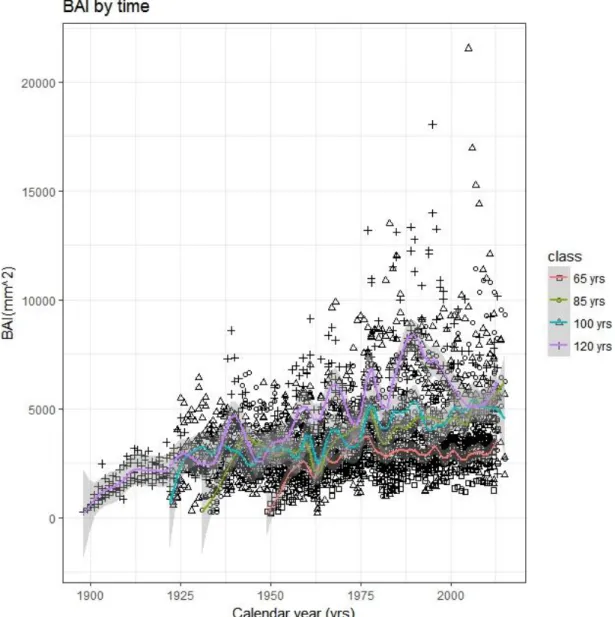
420 3 Results 421 3.1 Dendrochronology 422 423
All of the trees used in this study were satisfactorily cross-dated and no missing rings were 424
detected. The basal area increments of the different age classes are presented in Fig. 6 and Fig. 7, 425
along calendar year and along cambial age respectively. The general statistics of the tree-ring 426
chronologies are summarized in Table 3. The mean series inter-correlation (SI) that represents the 427
strength of the common signal shared by all series is about 0.5, while the expressed population 428
signal is above the conventional threshold (ESP>0.85) used to define the acceptability of the 429
chronology. This index confirms the goodness of cross-dating and the possibility to use this dataset 430
for further analysis. Furthermore, mean sensitivity (MS), which is an index of year-to-year 431
variability related to climate and/or disturbances, was also checked; a value ranking about 0.2 432
shows an adequate sensitive series, normally useful for climatic correlation analysis. 433
434
Tab.3| Descriptive statistics for raw (TRW) and ring width index (RWI) chronologies of the 4 different
age-classes. MW is mean ring width, SD is standard deviation, MS is mean sensitivity, AR1 the first order autocorrelation, ESP the expressed population signal, SI the series inter-correlation
TRW RWI
Age-class MW SD MS AR1 ESP SI
70 3.5484 1.6647 0.1488 0.8506 85 3.4193 2.0175 0.1871 0.855 100 3.605 1.7718 0.198 0.7519 120 3.3214 1.2572 0.2004 0.7088 total 3.495257 1.737886 0.181171 0.8034 0.855 0.50 435
436
Fig. 6 Time-related dynamics of basal area increments in different age-classes. Time series of basal area
437
increments (BAI), grouped by age-class and fitted with a cubic spline. The shaded areas indicate the
438
95% prediction interval of the function
440
Fig. 7 Diachronic analysis of age effects on basal area increments in different age-classes. Time
441
series of basal area increments (BAI), grouped by age-classes and fitted with a cubic spline. The shaded
442
areas indicate the 95% prediction interval of the spline function
443 444
3.2 Model output
445
In order to assess possible changes of growth rates over time, independent of the co-occurring 446
effects of ontogenetic factors, tree basal area increments (BAI) were modeled as: 447
ln(BAI) = f(AGE) + f(TIME) +εi (3)
448
where f(AGE) is the cambial age effect and f(TIME) represents all of the environmental effects 449
cumulated into a single global variable, varying over time. The BAI global long-term trend (Fig. 450
8b), after the subtraction of the age-related signal (Fig. 8a), shows an initial increase, two 451
culminations around the '30s and the '80s of the last century, a lower growth in between and a 452
subsequent decrease until the first decade of this century. The age-related effect displays the 453
expcted shape, with a steep increase at early age in the first part of the curve, followed by a less 454
pronounced growth, and an apparent culmination at an age of 100. 455
456
Fig. 8 GAM analysis of the independent effects on BAI of age and time.
457
a. Trend of basal area increments (BAI) as a function of age , after correcting for time-related effects. On
458
x-axis age (years), and on y-axis the function of age f(Age), dimensionless and centered around 0.
459
b. Global trend of BAI as a function of time , after correcting for age-related effects. On y-axis the
460
function of time s(TIME), dimensionless and centered around 0. Points represent partial residuals from
461
the fitted function and the shaded areas indicate the 95% prediction interval of fitted adaptive splines.
462
The GAM model was applied to log-transformed BAI data, so as to correct for heteroscedasticity.
463 464
Successively, in order to partition to individual drivers the effect so far attributed to global change, 465
seasonal climatic and geochemical variables were added to the model instead the time variable, and 466
after the backward stepwise variable selection, it was specified as follow: 467
ln(BAI) = f(Age) + f(CO2) + f(NOy dep) + f(SPEI JJA) + f(SPEI JJA t-1) + εi
468
Age is the age/size effect associated with variations in cambial age, CO2 is the annual level of
469
atmospheric [CO2], NOy depis the annual sum of dry and wet deposition of oxide N (NOy) species,
470
SPEI JJA and SPEI JJA t-1 represent the summer SPEI (Standardized Precipitation-471
Evapotranspiration Index; Vicente-Serrano et al. 2010) values in the ongoing and previous summer, 472
respectively. All variables exhibit a significant p-value at 0.001 level (Tab. 4), with a global 473
adjusted R2for the whole model of 0.371. 474
475
Tab. 4| Generalized additive model (GAM) results. Climatic and biological factors relationships with BAI
series (as a dependent variable) in Pseudotsuga menziesii. e.d.f. are effective degrees of freedom, F is the F-test for variance explained, P is the p-values and R2(adj) is the adjusted regression coefficient of the entire model.
Factor e.d.f. F P R2(adj)
Age 8.652 83.872 < 2e-16
CO2 7.172 14.951 < 2e-16
Noy dep 3.485 1.614 0.000705
SPEI JJA 1.961 3.513 4.80E-09
SPEI JJA t-1 1.757 2.16 5.25E-06
Whole model 0.371
477
Fig. 9. GAM analysis of increment response to individual drivers.Generalized additive models
478
(GAMs) results show the relationship between basal area increments (BAI) and environmental and
479
biological factors remaining after the backward selection procedure: cambial age, atmospheric [CO2] and 480
Standardized Precipitation Evapotranspiration Index computed over June , July and August of the current
481
year (SPEI JJA) and of the previous year (SPEI JJAt-1) . Values on the y-axis indicate the independent 482
effect of each covariate on basal area increments, as predicted by the model (continuous line)
483
dimensionless and centered around 0, plus the estimated degree of freedom (edf). Points represent partial
484
residuals from the fitted function and the shaded areas indicate the 95% prediction interval. The GAM
485
model was applied to log-transformed BAI data, so as to correct for heteroscedasticity.
486 487 488
4. Discussion
489
The primary purpose of this study was to assess if any changes in growth rates have occurred over 490
time in Douglas-fir in the northern Apennines, once correcting for age-related patterns. The global 491
long-term trend illustrates a decrease in the productivity of this species in the last four decades, 492
amounting to about 22.9%. These findings appear to be consistent with several other studies that 493
looked at forest growth changes in central Apennines (Piovesan et al. 2008), in the Mediterranean 494
region by and large (Linares et al.,2010) and in other European areas (Vitas and Žeimavičius 2006). 495
All of these studies found that the increase in summer drought had a negative effect on growth, in 496
association with co-varying factors, such as stand dynamics, competition and/or pests. These could 497
exacerbate the role of the imbalance in water availability and overcome the potentially positive 498
effects of atmospheric nitrogen deposition, of the increase in the length of the growing season, and 499
of the rise in atmosphere [CO2]. The general trend recorded in this study can be partially explained
500
by examining the shape of the relationship between significant environmental factors and BAI. The 501
response to atmospheric [CO2] (Fig. 9b) presents a strong positive pattern at the low end of the
502
concentration range, with a culmination at around 310 ppm, followed by a decline and an apparent 503
lack of effect at higher concentrations. Although the lack of evidence of a clear fertilization effect 504
of CO2is in agreement with previous studies (Peñuelas et al. 2011; Lévesque et al. 2014), it could
505
lead to different conclusions, depending on the processes involved. In a biological perspective, for 506
example, both long-term photosynthetic acclimation (Medlyn et al. 1999) and a shift in allocation 507
of assimilated C to faster-turnover pools such as fine roots or canopy foliage (Korner et al., 2005) 508
are possible explanations. Moreover, this lack of response could be the result of an interaction 509
between CO2 and nutrient availability effects, which cannot be accounted by a simple additive
510
model. Finally, such a apparent saturation effect of CO2could be the result of the lack of significant
511
variables, not included in the model, as for example inter-tree competition. Indeed the radial 512
growth of shade intolerant trees is very much dependent on forest management practices, especially 513
in even-aged stands. Moreover, the extent of drought events could have been insufficiently 514
represented by the rather crude approach applied in the study. Summer water availability (Figure 515
9d), which is related to the transpiration demand, is the second most important variable affecting the 516
behavior of this species in the long-term, conditioning its growth performance (Beedlow et al. 517
2013) and distribution (Rehfeldt et al. 2014). Air dryness, which is also known to affect Douglas fir, 518
was not included as a potential driver due to a lack of suitable information. Furthermore, the 519
influence of the previous growing seasons’ summer water balance (Figure 9e) also affects the
520
growth trend, as early-wood width is related to the amount of carbon storage reserves built-up in the 521
preceding year, which are subject to remobilisation in the first phase of vegetative growth (Lee et al. 522
2016). At last, our findings suggest a positive relationship between growth and N deposition 523
(Figure 9c), which potentially reflects the beneficial effect of N increase on photosynthetic rates due 524
to the resulting increase in photosynthetic pigments as well as Rubisco foliar content. The possible 525
stabilization observed at the higher rate of N deposition, if significant, could be interpreted as a 526
saturation of the nitrogen effect on the system. Although N-mineralisation rates at the site are not 527
known, such a saturation above a deposition a N deposition rate of 4.5 kg /ha/yr, however, seems 528
unlikely since Douglas-fir soils at the site display rather high C:N ratios, with an average value of 529
27 (Di Biase et al. 2015), although N mineralisation data are not available to support such the 530
hypothesis of substantial N limitations. Besides, N uptake by Douglas-fir was found to increase 531
asymptotically, until at least 35 kg N ha-1yr-1of net nitrogen available (Perakis and Sinkhorn 2011) 532
in US Pacific Coast environments. A possible influence caused by concurvity with other factors, 533
namely CO2 concentration, should be also taken into consideration. Indeed, when non-stationary
534
forcing factors (i.e., atmospheric [CO2] and nitrogen deposition) co-vary, it is difficult to
535
disentangle their individual effects on long-term tree growth, and this complication increases with 536
the complexity of the model (Carrer and Urbinati 2006). 537
5 Conclusions
538
Given the importance of Douglas-fir as a timber species, the ongoing decrease in growth 539
performance illustrated by this study for the northern Apennines could have relevant implications 540
from a management perspective. For this reason, understanding which factors have been 541
determining such a trend is particularly important. Our model, despite the rather low amount of 542
variance explained and the simplicity of the model structure (only few variables considered), as 543
well as its additive nature, allows us to draw some conclusions. The impact of summer water 544
availability, which is projected to decrease in the Mediterranean region (IPCC, 2014), could be 545
responsible to a considerable extent for the observed decrease in growth rates in recent decades, due 546
to the increase in magnitude and frequency of drought events. A parallel positive effect ascribable 547
to N deposition, which should have promoted the stem growth in the past, may no longer be able to 548
counterbalance the summer drought stress effect, due to the stabilization in NOy emission and an 549
apparent saturation of the N response. Especially in the absence of a positive effect of fertilization 550
by rising atmospheric [CO2], the observed trend can be expected to be exacerbated in the next
551
future. 552
Finally, GAMs appear to have a promising potential to disentangle non-linear biological and 553
environmental effects affecting tree growth, resulting in long-term trend preservation, which is 554
fundamental if a better understanding of past environmental effects is to be used to understand the 555
future behavior of forests in a changing world. 556
6.Acknowledgments
557
We thank NOAA (ITRDB and ESRL) and the Regional Hydrological Service of the Tuscany 558
Region (SIR), for providing the data used in this study; also the “Reparto Carabinieri per la 559
biodiversità di Vallombrosa” which kindly provided sampling permission. 560
This work was carried out within the framework of the Convention between the Department of 561
Agricultural Sciences of the University of Bologna and the Council for Agricultural Research and 562
Economics. 563
564
7. Bibliography
565
ABER, JOHN D., CHRISTINE L. GOODALE, SCOTT V. OLLINGER, MARIE-LOUISE 566
SMITH, ALISON H. MAGILL, MARY E. MARTIN, RICHARD A. HALLETT, and JOHN 567
L. STODDARD. 2003. “Is Nitrogen Deposition Altering the Nitrogen Status of Northeastern
568
Forests?” BioScience 53 (4): 375. doi:10.1641/0006-3568(2003)053[0375:INDATN]2.0.CO;2.
569
Aho, Ken, DeWayne Derryberry, and Teri Peterson. 2014. “Model Selection for Ecologists: The
570
Worldview of AIC and BIC.” Ecology 95 (March): 631–36. doi:10.1890/13-1452.1.
Ainsworth, Elizabeth A., and Stephen P. Long. 2005. “What Have We Learned from 15 Years of
572
Free-Air CO2 Enrichment (FACE)? A Meta-Analytic Review of the Responses of 573
Photosynthesis, Canopy Properties and Plant Production to Rising CO2.” New Phytologist 165 574
(2): 351–71. doi:10.1111/j.1469-8137.2004.01224.x. 575
Babst, Flurin, M. Ross Alexander, Paul Szejner, Olivier Bouriaud, Stefan Klesse, John Roden, 576
Philippe Ciais, et al. 2014. “A Tree-Ring Perspective on the Terrestrial Carbon Cycle.”
577
Oecologia 176 (2): 307–22. doi:10.1007/s00442-014-3031-6. 578
Beedlow, Peter A., E. Henry Lee, David T. Tingey, Ronald S. Waschmann, and Connie A. Burdick. 579
2013. “The Importance of Seasonal Temperature and Moisture Patterns on Growth of
Douglas-580
Fir in Western Oregon, USA.” Agricultural and Forest Meteorology 169. Elsevier B.V.: 174– 581
85. doi:10.1016/j.agrformet.2012.10.010. 582
Biondi, Franco. 1999. “Comparing Tree-Ring Chronologies and Repeated timberiInventories as
583
Forest Monitoring Tools.” Ecological Applications 9 (1): 216–27.
doi:10.1890/1051-584
0761(1999)009[0216:CTRCAR]2.0.CO;2. 585
Boettger, Tatjana, Marika Haupt, Kay Knöller, Stephan M. Weise, John S. Waterhouse, Katja T. 586
Rinne, Neil J. Loader, et al. 2007. “Wood Cellulose Preparation Methods and Mass
587
Spectrometric Analyses of ??13C, ??18O, and Nonexchangeable ??2H Values in Cellulose, 588
Sugar, and Starch: An Interlaboratory Comparison.” Analytical Chemistry 79 (12): 4603–12.
589
doi:10.1021/ac0700023. 590
Boisvenue, Céline, and Steven W. Running. 2006. “Impacts of Climate Change on Natural Forest
591
Productivity - Evidence since the Middle of the 20th Century.” Global Change Biology 12 (5): 592
862–82. doi:10.1111/j.1365-2486.2006.01134.x. 593
Brienen, R J W, E Gloor, S Clerici, R Newton, L Arppe, A Boom, S Bottrell, et al. n.d. “Isotopes.” 594
Nature Communications. Springer US, 1–10. doi:10.1038/s41467-017-00225-z. 595
Brunel, J.P., G.R. Walker, C.D. Walker, J.C. Dighton, and A. Kennett-Smith. 1991. “Using Stable 596
Isotopes of Water to Trace Plant Water Uptake.” International Symposium on the Use of Stable
597
Isotopes in Plant Nutrition, Soil Fertility and Environmental Studies, 543–551. 598
doi:10.2144/000114133. 599
Bunn, Andrew G. 2008. “A Dendrochronology Program Library in R (dplR).” Dendrochronologia
600
26 (2): 115–24. doi:10.1016/j.dendro.2008.01.002. 601
Camarero, J. Julio, Antonio Gazol, Jacques C. Tardif, and France Conciatori. 2015. “Attributing 602
Forest Responses to Global-Change Drivers: Limited Evidence of a CO2-Fertilization Effect in 603
Iberian Pine Growth.” Journal of Biogeography 42 (11): 2220–33. doi:10.1111/jbi.12590.
604
Carrer, Marco, and C Urbinati. 2006. “Long-Term Change in the Sensitivity of Tree‐ring Growth
605
to Climate Forcing in Larix Decidua.” New Phytologist 170 (iv): 861–72. 606
Cook, Edward R., Keith R. Briffa, David M Meko, Donald A Graybill, and Gary Funkhouser. 1995. 607
“The ’segment Length Curse’ in Long Tree-Ring Chronology Development for Palaeoclimatic
608
Studies.” The Holocene 5 (2): 229–37. doi:10.1177/095968369500500211.
609
Dawson, T E. 1998. “ Fog in the Californian Redwood Forest: Ecosystem Inputs and Use by
610
Plants.” Oecologia 117: 476–85.
611
Dawson, Todd E., Stefania Mambelli, Agneta H. Plamboeck, Pamela H. Templer, and Kevin P. Tu. 612
2002. “Stable Isotopes in Plant Ecology.” Annual Review of Ecology and Systematics 33 (1): 613
507–59. doi:10.1146/annurev.ecolsys.33.020602.095451. 614
Dawson, Todd E., and John S Pate. 1996. “Seasonal Water Uptake and Movement in Root Systems
615
of Australian Phraeatophytic Plants of Dimorphic Root Morphology: A Stable Isotope 616
Investigation.” Oecologia 107 (1): 13–20. doi:10.1007/BF00582230.
617
Di Biase, Giampaolo, Gloria Falsone, Anna Graziani, Gilmo Vianello, and Livia Vittori Antisari. 618
2015. “Carbon Sequestration in Soils Affected By Douglas Fir Reforestation in Apennines
619
(Northern Italy).” Eqa-International Journal of Environmental Quality 17: 1–11.
620
doi:10.6092/issn.2281-4485/5208. 621
Dongmann, G, and H W Nürnberg. 1974. “On the Enrichment of H2180 in the Leaves of
622
Transpiring Plants I T L Q E” 52: 1–2.
623
Esper, Jan, Edward R Cook, and Fritz H Schweingruber. 2002. “Low-Frequency Signals in Long
624
Tree-Ring Chronologies for Reconstructing Past Temperature Variability.” Science (New York, 625
N.Y.) 295 (5563). American Association for the Advancement of Science: 2250–53. 626
doi:10.1126/science.1066208. 627
Esper, Jan, David C. Frank, Giovanna Battipaglia, Ulf Büntgen, Christopher Holert, Kerstin 628
Treydte, Rolf Siegwolf, and Matthias Saurer. 2010a. “Low-Frequency Noise in δ13C and
629
δ18O Tree Ring Data: A Case Study of Pinus Uncinata in the Spanish Pyrenees.” Global
630
Biogeochemical Cycles 24 (4): 1–11. doi:10.1029/2010GB003772. 631
Esper, Jan, David C Frank, Giovanna Battipaglia, Ulf Büntgen, Christopher Holert, Kerstin Treydte, 632
Rolf Siegwolf, and Matthias Saurer. 2010b. “Low ‐ Frequency Noise in D 13 C and D 18 O
633
Tree Ring Data : A Case Study of Pinus Uncinata in the Spanish Pyrenees” 24 (2): 1–11. 634
doi:10.1029/2010GB003772. 635
Farquhar, G. D., L. A. Cernusak, and B. Barnes. 2006. “Heavy Water Fractionation during
636
Transpiration.” Plant Physiology 143 (1): 11–18. doi:10.1104/pp.106.093278.
637
Farquhar, G D, J R Ehleringer, and K T Hubick. 1989. “Carbon Isotope Discrimination and 638
Photosynthesis.” Annual Review of Plant Physiology and Plant Molecular Biology.
639
doi:10.1146/annurev.pp.40.060189.002443. 640
Federal, Swiss, Universitat De Barcelona, J. Julio Camarero, Antonio Gazol, Juan Diego Galván, 641
Gabriel Sangüesa-Barreda, and Emilia Gutiérrez. 2015. “Disparate Effects of Global-Change 642
Drivers on Mountain Conifer Forests: Warming-Induced Growth Enhancement in Young Trees 643
vs. CO 2 Fertilization in Old Trees from Wet Sites.” Global Change Biology 21 (2): 738–49. 644
doi:10.1111/gcb.12787. 645
Fenn, Mark E, Jeremy S Fried, Haiganoush K Preisler, Andrzej Bytnerowicz, Susan Schilling, 646
Sarah Jovan, and Olaf Kuegler. 2015. “REMEASURED FIA PLOTS REVEAL TREE-LEVEL
647
DIAMETER GROWTH AND TREE MORTALITY IMPACTS OF NITROGEN 648
DEPOSITION ON CALIFORNIA ’ S FORESTS” 2013 (Time 2): 2013–16.
649
Francey, R. J., C. E. Allison, D. M. Etheridge, C. M. Trudinger, I. G. Enting, M. Leuenberger, R. L. 650
Langenfelds, E. Michel, and L. P. Steele. 1999. “A 1000-Year High Precision Record of δ13C
651
in Atmospheric CO2.” Tellus, Series B: Chemical and Physical Meteorology 51 (2): 170–93.
652
doi:10.1034/j.1600-0889.1999.t01-1-00005.x. 653
Frank, D. C., B. Poulter, M. Saurer, J. Esper, C. Huntingford, G. Helle, K. Treydte, et al. 2015. 654
“Water-Use Efficiency and Transpiration across European Forests during the Anthropocene.”
655
Nature Climate Change, no. May. doi:10.1038/nclimate2614. 656
Giustini, Francesca, Mauro Brilli, and Antonio Patera. 2016. “Mapping Oxygen Stable Isotopes of 657
Precipitation in Italy.” Journal of Hydrology: Regional Studies 8. Elsevier B.V.: 162–81. 658
doi:10.1016/j.ejrh.2016.04.001. 659
Gómez-Guerrero, Armando, Lucas C.R. R Silva, Miguel Barrera-Reyes, Barbara Kishchuk, 660
Alejandro Velázquez-Martínez, Tomás Martínez-Trinidad, Francisca Ofelia Plascencia-661
Escalante, and William R. Horwath. 2013. “Growth Decline and Divergent Tree Ring Isotopic
662
Composition (δ13C and δ18O) Contradict Predictions of CO2 Stimulation in High Altitudinal
663
Forests.” Global Change Biology 19 (6): 1748–58. doi:10.1111/gcb.12170.
664
Griffin, Daniel, and Kevin J Anchukaitis. 2014. “How Unusual Is the 2012 – 2014 California
665
Drought ?,” 9017–23. doi:10.1002/2014GL062433.1. 666
Guerrieri, R, Maurizio Mencuccini, L J Sheppard, M Saurer, M P Perks, P Levy, M a Sutton, Marco 667
Borghetti, and J Grace. 2011. “The Legacy of Enhanced N and S Deposition as Revealed by 668
the Combined Analysis of Delta 13C, Delta 18O and Delta 15N in Tree Rings.” Global
669
Change Biology 17 (5): 1946–62. doi:10.1111/j.1365-2486.2010.02362.x. 670
Harris, I., P. D. Jones, T. J. Osborn, and D. H. Lister. 2014. “Updated High-Resolution Grids of 671
Monthly Climatic Observations - the CRU TS3.10 Dataset.” International Journal of 672
Climatology 34 (3): 623–42. doi:10.1002/joc.3711. 673
Hastie, T. J., and R. J. Tibshirani. 1990. “Generalized Additive Models.” Monographs on Statistics 674
and Applied Probability. doi:10.1016/j.csda.2010.05.004. 675
IPCC. 2014. “Climate Change 2014 Synthesis Report Summary Chapter for Policymakers.” Ipcc,
676
31. doi:10.1017/CBO9781107415324. 677
Keenan, Trevor F, David Y Hollinger, Gil Bohrer, Danilo Dragoni, J William Munger, Hans Peter 678
Schmid, and Andrew D Richardson. 2013. “Increase in Forest Water-Use Efficiency as
679
Atmospheric Carbon Dioxide Concentrations Rise.” Nature 499 (7458): 324–27.
680
doi:10.1038/nature12291. 681
Korner, C. 2005. “Carbon Flux and Growth in Mature Deciduous Forest Trees Exposed to Elevated
682
CO2.” Science 309 (5739): 1360–62. doi:10.1126/science.1113977.
683
Leavitt, Steven W. 2010. “Tree-Ring C-H-O Isotope Variability and Sampling.” The Science of the
684
Total Environment 408 (22): 5244–53. doi:10.1016/j.scitotenv.2010.07.057. 685
Lee, E. Henry, Peter A. Beedlow, Ronald S. Waschmann, David T. Tingey, Charlotte Wickham, 686
Steve Cline, Michael Bollman, and Cailie Carlile. 2016. “Douglas-Fir Displays a Range of
687
Growth Responses to Temperature, Water, and Swiss Needle Cast in Western Oregon, USA.”
688
Agricultural and Forest Meteorology 221. Elsevier B.V.: 176–88. 689
doi:10.1016/j.agrformet.2016.02.009. 690
Leonardi, Stefano, Tiziana Gentilesca, Rossella Guerrieri, Francesco Ripullone, Federico Magnani, 691
Maurizio Mencuccini, Twan V. Noije, and Marco Borghetti. 2012. “Assessing the Effects of 692
Nitrogen Deposition and Climate on Carbon Isotope Discrimination and Intrinsic Water-Use 693
Efficiency of Angiosperm and Conifer Trees under Rising CO 2 Conditions.” Global Change 694
Biology 18 (9): 2925–44. doi:10.1111/j.1365-2486.2012.02757.x. 695
Lévesque, Mathieu, Rolf Siegwolf, Matthias Saurer, Britta Eilmann, and Andreas Rigling. 2014. 696
“Increased Water-Use Efficiency Does Not Lead to Enhanced Tree Growth under Xeric and
697
Mesic Conditions.” New Phytologist 203 (1): 94–109. doi:10.1111/nph.12772.
698
Linares, Juan Carlos, Jesús Julio Camarero, and José Antonio Carreira. 2010. “Competition
699
Modulates the Adaptation Capacity of Forests to Climatic Stress: Insights from Recent Growth 700
Decline and Death in Relict Stands of the Mediterranean Fir Abies Pinsapo.” Journal of
701
Ecology 98 (3): 592–603. doi:10.1111/j.1365-2745.2010.01645.x. 702
Magnani, Federico, Maurizio Mencuccini, Marco Borghetti, Paul Berbigier, Frank Berninger, 703
Sylvain Delzon, Achim Grelle, et al. 2007. “The Human Footprint in the Carbon Cycle of 704
Temperate and Boreal Forests.” Nature 447 (7146): 848–50. doi:10.1038/nature05847.
705
Marshall, D D, and R O Curtis. 2002. “Levels-of-Growing-Stock Cooperative Study in
Douglas-706
Fir: Report No. 15 - Hoskins: 1963-1998.” Research Paper Pacific Northwest Research 707
Station, USDA Forest Service, no. PNW-RP-537: 80. 708
McCarroll, Danny, and Neil J. Loader. 2004. “Stable Isotopes in Tree Rings.” Quaternary Science
709
Reviews 23 (7–8): 771–801. doi:10.1016/j.quascirev.2003.06.017. 710
McMahon, Sean M, Geoffrey G Parker, and Dawn R Miller. 2010. “Evidence for a Recent Increase
711
in Forest Growth.” Proceedings of the National Academy of Sciences of the United States of
712
America 107 (8): 3611–15. doi:10.1073/pnas.0912376107. 713
Medlyn, B. E., F. -W. Badeck, D. G. G. De Pury, C. V. M. Barton, M. Broadmeadow, R. 714
Ceulemans, P. De Angelis, et al. 1999. “Effects of Elevated [CO2] on Photosynthesis in
715
European Forest Species: A Meta-Analysis of Model Parameters.” Plant, Cell & Environment 716
22 (12): 1475–1495. doi:10.1046/j.1365-3040.1999.00523.x. 717
Nair, Richard K F, Micheal P Perks, Andrew Weatherall, Elizabeth M Baggs, and Maurizio 718
Mencuccini. 2015. “Does Canopy Nitrogen Uptake Enhance Carbon Sequestration by Trees?”
719
Global Change Biology, September. doi:10.1111/gcb.13096. 720
Nehrbass-Ahles, Christoph, Flurin Babst, Stefan Klesse, Magdalena Nötzli, Olivier Bouriaud, 721
Raphael Neukom, Matthias Dobbertin, and David Frank. 2014. “The Influence of Sampling
722
Design on Tree-Ring-Based Quantification of Forest Growth.” Global Change Biology 20 (9). 723
doi:10.1111/gcb.12599. 724
Norby, Richard J, Jeffrey M Warren, Colleen M Iversen, Belinda E Medlyn, and Ross E 725
McMurtrie. 2010. “CO2 Enhancement of Forest Productivity Constrained by Limited Nitrogen
726
Availability.” Proceedings of the National Academy of Sciences of the United States of
727
America 107 (45): 19368–73. doi:10.1073/pnas.1006463107. 728
Peñuelas, Josep, Josep G. Canadell, and Romà Ogaya. 2011. “Increased Water-Use Efficiency
729
during the 20th Century Did Not Translate into Enhanced Tree Growth.” Global Ecology and
730
Biogeography 20 (4): 597–608. doi:10.1111/j.1466-8238.2010.00608.x. 731
Perakis, Steven S., and Emily R. Sinkhorn. 2011. “Biogeochemistry of a Temperate Forest Nitrogen
732
Gradient.” Ecology 92 (7): 1481–91. doi:10.1890/10-1642.1.
733
Peters, Richard L., Peter Groenendijk, Mart Vlam, and Pieter a. Zuidema. 2015. “Detecting
Long-734
Term Growth Trends Using Tree Rings: A Critical Evaluation of Methods.” Global Change
735
Biology, n/a-n/a. doi:10.1111/gcb.12826. 736