A DIVIDE-ET-IMPERA APPROACH TO PATH PLANNING FOR GROUND COVERING WITH AN UAV
Supervisor:
Prof. Francesco AMIGONI
Master Thesis by: Simone BIANCHI Student ID 883360
tions, covering of ocean floors.CPP problems are known to be NP-hard. Due to this, optimal solutions are approximated using various methods.In particular, the problem addressed in this thesis is to cover a 2D area at the ground by solving multiple CPPs over 2D grids, that are obtained as the result of the intersection of the 3D environment with |H| horizontal planes at different heights h ∈ H, where H denotes the set of discrete heights. The UAV uses a sensor with a conic FOV (Field Of View) that is used to cover the ground.
Our main goal is to reduce the computational cost in a CPP problem. To do this, we adopt a divide-et-impera approach. In computer science, divide-et-impera is a method that consists in dividing the initial problem into two or more simple sub-problems. After that, the solutions of the sub-problems must be combined to obtain the final result. In our case, we divide the entire environment in smaller sections that are covered separately through the Art Gallery Problem (AGP) as a set cover problem in order to find a feasible set of covering points (from which the target area can be fully covered) and the Travel Salesman Problem (TSP) to connect them. After the paths over all the zones are produced, a merge algorithm obtains the final single path that covers the entire target surface.
We introduce two different merge algorithms. The first one solves the problem more rapidly in terms of computational time but generally produces high cost paths, vice versa the second one produces paths with less cost than the first al-gorithm at the expense of a higher computational time. We implement these algorithms in three different environments and with different FOVs (Field Of Views) of the UAV sensor. Then we compare the results obtained with the results obtained without a divide-et-impera approach.
3D, e il controllo delle semine in agricoltura. Il problema del CPP `e NP-hard, per questo motivo vengono proposte soluzioni che approssimano il risultato ottimo. In questa tesi trattiamo il problema di copertura di un’area al suolo come una composizione di pi`u problemi di copertura 2D, poich´e suddividiamo l’ambiente 3D in |H| sezioni orizzontali a diverse altezze prestabilite h ∈ H, dove H `e l’insieme discreto delle altezze. L’UAV utilizza un sensore con un FOV (Field Of Viewe) conico usato per coprire il terreno.
Il nostro obiettivo principale `e quello di ridurre il costo computazionale nei pro-blemi di CPP. Per fare questo utiliazziamo un approccio divide-et-impera. In informatica, tale approccio prevede la suddivisione del problema iniziale in uno o pi`u sottoproblemi pi`u semplici. Successivamente, le soluzioni dei sottoproblemi devono essere combinate a formare la soluzione del problema iniziale. Nel nostro caso, dividiamo l’intera mappa in diverse zone pi`u piccole che vengono coperte separatamente. Nel nostro caso, la copertura viene effettuata da un Art Gallery Problem (AGP), un problema di set cover il cui obiettivo `e quello di trovare un insieme di punti di copertura che coprano l’intera area di interesse. Successiva-mente, il Problema del Commesso Viaggiatore (TSP) viene utilizzato per trovare un tour che connetta i punti di copertura individuati. Dopo aver ottenuto i per-corsi di copertura di tutte le zone, un algoritmo di unione produce il risultato finale.
Due algoritmi di unione vengono proposti nella tesi. Il primo produce risultati con un minore tempo computazionale ma generalmente produce percorsi costosi per quanto riguarda la distanza, viceversa, il secondo algoritmo ha con un costo computazionale pi`u elevato ma minori costi di distanza. Implementiamo questi due algoritmi di unione su diversi ambienti e con differenti FOV (Field Of View) del sensore dell’UAV. Infine analizziamo e compariamo i risultati ottenuti met-tendoli a confronto con i risultati ottenuti senza un approccio divide-et-impera.
Desidero ringraziare il Professor Francesco Amigoni per la disponibilit`a mostra-tami e per gli utili consigli datomi durante questi ultimi mesi.
Ringrazio la mia famiglia, in particolare i miei genitori Beatrice e Marco per avermi sostenuto economicamente durante questi anni sia economicamente che moralmente nei momenti pi`u stressanti e in quelli pi`u gioiosi. Un ringraziamento particolare va a mio pap`a Paolo che mi ha trasmesso la passione per la tecnologia sin da bambina e senza di cui non avrei mai intrapreso questa strada. Ringrazio anche mio zio Flavio che mi ha sempre accompagnata, letteralmente, in questi anni.
Ringrazio Laura per esserci sempre stata nei momenti belli e in quelli pi`u tristi, per avermi sempre rallegrato dopo un insuccesso e per avermi sempre spronato ad affrontare qualsiasi difficolt`a con sicurezza e a credere nelle mie capacit`a.
Infine, ringrazio i miei colleghi universitari che hanno reso pi`u divertente e piacevole questo percorso.
Abstract I
Sommario II
Ringraziamenti IV
1 Introduction 1
1.1 Structure of the Thesis . . . 3
2 State of the Art 4 2.1 Introduction to CPP . . . 4 2.2 2D Coverage . . . 5 2.3 3D Coverage . . . 11 2.4 Multi-UAV Coverage . . . 21 3 Problem Setting 24 3.1 Problem Statement . . . 24 3.2 Problem Analysis . . . 27 4 Algorithms 30 4.1 First step process methods . . . 30
4.1.1 Art Gallery Problem . . . 30
4.1.2 A* and Theta* algorithms . . . 31
4.1.3 Travelling Salesman Problem . . . 34
4.2 The Coverage Algorithms . . . 35
4.2.1 SingleHeight Algorithm . . . 35
4.2.2 TwoHeights Algorithm . . . 36
4.3 Second step process - Merge algorithms . . . 37
4.3.1 First Merge Algorithm . . . 37
6 Conclusions and future works 61
A Occupancy grid maps in all the three environments 63
B Optimal paths maps for all the environments and different FOVs 67
2.1 Summary of 2D works presented. . . 11
2.2 Summary of 3D works presented. . . 22
2.3 Summary of multi-robot works presented. . . 23
5.1 Matrix size of each 2D occupancy grid map. . . 44
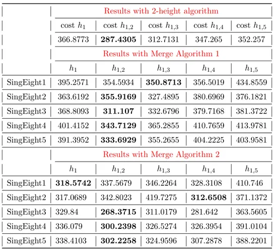
5.2 Comparison of results of Environment A and α = 60◦ . . . 47
5.3 Comparison of results of Environment A and α = 85◦ . . . 48
5.4 Comparison of results of Environment B and α = 60◦ . . . 51
5.5 Comparison of results of Environment B and α = 85◦ . . . 52
5.6 Comparison of results of Environment C and α = 60◦ . . . 55
5.7 Comparison of results of Environment C and α = 85◦ . . . 56
5.8 The minimum-cost coverage tour found by the Merge Algorithm 1 the heights merged and their computational time. . . 58
5.9 The minimum-cost coverage tour found by the Merge Algorithm 2 the heights merged and their computational time. . . 59
5.10 The minimum-cost coverage tour found by the Merge Algorithm 2 the heights merged and their computational time. . . 60
which the slices are circles. Rather than moving along circular paths and stepping outward, the robot follows a spiral pattern [1]. 6 2.3 An example of wavefront path [44]. . . 7 2.4 (a) (b) A solution using Spiral STC algorithm [18]. . . 8 2.5 (a) Optimal tour when travelling time is minimized first [3]. (b)
Optimal tour when sensing time is minimized first [3]. . . 9 2.6 (a) The robot will cover area A with boundary B [26]. (b) At the
top is shown a cross section in the plane y = y0, P1, P2 and P3 are points where the surface exceed the threshold slope µ. In the bottom the area A is projected onto the 2D plane [26]. (c) Shows the path of the robot starting from SP [26]. . . 12 2.7 Hemispherical simplification of urban structure and hemispherical
trajectory of UAV [9] . . . 13 2.8 Sampling scheme and its dual scheme proposed by Latombe and
Gonzalez-Banos to solve a variation of the AGP [23]. . . 14 2.9 Stateflow diagram illustrating two algorithms based on CSP [16]. . 15 2.10 Path generated by the Cone-TSPN algorithm [33]. . . 16 2.11 (a) Workplace identification [41]. (b)Coverage trajectory generated
[41]. (c) Mosaic reconstruction [41]. . . 17 2.12 (a) Grid-based decomposition [31]. (b)Optimal path generated by
wavefront algorithm [31]. (c) Coverage trajectory generated by cubic interpolation [31]. . . 18 2.13 (a) Coverage path of the planar region [19]. (b)Coverage path
planning of the high slopes [19]. (c) Diagram of the coverage path-planning algorithm for bathymetric maps. [19]. . . 19
to grids in different resolutions [36]. . . 20 2.15 Flowchart of the system proposed by Barrientos et al. [4]. . . 21 3.1 (a) Example of 3D decomposition in different planes [2]. (b)
Ex-ample of the FOV varying with height [2]. . . 25 3.2 Examples of (a) Type 1 (b) Type 2 . . . 27 3.3 Division of the entire map in two 3D-zones. On the left a type 1
environment, on the right a type 2 one. . . 28 4.1 A* grid path versus true shortest path [12]. . . 32 4.2 Examples of (a) Two different paths (b) Paths merged using the
first algorithm . . . 39 4.3 Examples of (a) Two different paths (b) Paths merged using the
second algorithm with strategy 1 . . . 41 5.1 The 3 target regions at the ground used during the experiments. . 43 5.2 Decomposition of a 3D environment in six grids of Environment C
in Case 1. . . 45 5.3 Target ground division of the Environment A,B,C. . . 46 5.4 Computational time of execution of the algorithm in Environment
B with different FOVs . . . 48 5.5 The coverage tours of Environment A with a α = 85◦. It shows the
paths before the merge. (a) Tour at h2with SingleHeight algorithm for the type 1 area. (b) Tour at h2 with the TwoHeight on the type 2 area. . . 49 5.6 The coverage tours of Environment A with a α = 85◦. (a) Tour
at h2 with Merge Algorithm 1. (b) Tour at h2 with the Merge Algorithm 2. (c) Tour at h3 with the Merge Algorithm 2. . . 50 5.7 The coverage tours of Environment B with a α = 60◦. It shows the
paths before the merge. (a) Tour at h5with SingleHeight algorithm for the type 1 area. (b) Tour at h1 with the TwoHeight on the type 2 area. (c) Tour at h4 with the TwoHeight on the type 2 area. . . 52 5.8 The coverage tour of Environment B with a α = 60◦ computed
with Merge Algorithm 1. The height are in ascending order. (a) Tour at h1. (b) Tour at h4. (c) Tour at h5. . . 53 5.9 The coverage tour of Environment B with a α = 60◦ computed
with Merge Algorithm 2. The height are in ascending order. (a) Tour at h1. (b) Tour at h3. (c) Tour at h5. . . 53 5.10 Computational time of execution of the algorithm in Environment
A.1 Six grids represent the occupancy grid maps at different heights of Environment A in ascending order starting from h0 (the ground) to h5. Also the division is showed. . . 64 A.2 Six grids represent the occupancy grid maps at different heights of
Environment B in ascending order starting from h0 (the ground) to h5. Also the division is showed. . . 65 A.3 Six grids represent the occupancy grid maps at different heights of
Environment C in ascending order starting from h0 (the ground) to h5. Also the division is showed. . . 66 B.1 The coverage tours of Environment A with a α = 60◦. (a) Tour
at h1 with Merge Algorithm 1. (b) Tour at h4 with the Merge Algorithm 1. (c) Tour at h5 with the Merge Algorithm 1. (d) Tour at h1 with Merge Algorithm 2. (e) Tour at h4 with the Merge Algorithm 2. (f) Tour at h5 with the Merge Algorithm 2. . . 68 B.2 The coverage tours of Environment A with a α = 85◦. (a) Tour
at h2 with Merge Algorithm 1. (b) Tour at h2 with the Merge Algorithm 2. (c) Tour at h3 with the Merge Algorithm 2. . . 69 B.3 The coverage tour of Environment B with a α = 60◦ computed. (a)
Tour at h1 with Merge Algorithm 1. (b) Tour at h4 with Merge Algorithm 1. (c) Tour at h5 with Merge Algorithm 1. (d) Tour at h1 with Merge Algorithm 2. (e) Tour at h3 with Merge Algorithm 2. (f) Tour at h5 with Merge Algorithm 2. . . 70 B.4 The coverage tour of Environment B with a α = 85◦ computed. (a)
Tour at h1 with Merge Algorithm 1. (b) Tour at h5 with Merge Algorithm 1. (c) Tour at h1 with Merge Algorithm 2. (d) Tour at h2 with Merge Algorithm 2. . . 71 B.5 The coverage tour of Environment C with a α = 60◦ computed.(a)
Tour at h1 with Merge Algorithm 1. (b) Tour at h4 with Merge Algorithm 1. (c) Tour at h5 with Merge Algorithm 1. (d) Tour at h1 with Merge Algorithm 2. (e) Tour at h5 with Merge Algorithm 2. 72
Algorithm 1. (c) Tour at h3 with Merge Algorithm 1. (d) Tour at h1 with Merge Algorithm 2. (e) Tour at h2 with Merge Algorithm 2. (f) Tour at h4 with Merge Algorithm 2. . . 73
Travelling Salesman Problem (TSP) Neighborhoods-TSP (TSPN)
Field of view (FOV)
Coverage sampling problem (CSP) Probabilistic Roadmaps (PRM)
Introduction
The applications of UAVs (Unmanned Aerial Vehicles) have increased over the last years. While they originated mostly in military applications, their use has rapidly expanded to leisure activities, such as photography and videography, ap-plications in industrial inspection [6], in agriculture (in precision agriculture for crop, soil, and irrigation monitoring) [4, 40] and for the inspection of buildings. Also, another type of robots, called AUV (Autonomous Underwater Vehicle) are used to cover seafloors [1,19]. The advantages of UAVs and AUVs are: lower risks for humans and more efficiency and precision in performing the tasks.
In the field of autonomous robot planning, the Coverage Path Planning (CPP) problem is a well studied problem. It consists of finding a path that covers a target area avoiding obstacles. The space may be represented in different ways [1,10,42,44] and the paths can be computed using different methods [18,35,43,44]. Aiming to cover 3D environments, a number of algorithms have been recently pro-posed [20,26]. Some methods are based on a two-step optimization process and are independent from any specific scenario. In the first phase, an AGP (Art Gallery Problem) is solved, which consists of finding the minimal set of viewpoints (called covering points) from which the whole target space can be covered. In the second phase a Travelling Salesman Problem (TSP) is solved, and the shortest tour con-necting the covering points is computed. [3, 39] propose a two-phase optimization methods using MILP (Mixed Integer Linear Programming) for solving a CPP in 2D environments. Due to the fact that both the AGP and the TSP are NP-hard, fast algorithms that provide approximate solutions are used in many works to solve these two problems: for istance Latombe and Gonzalez-Banos in [22, 23] propose two approximation solutions to solve the AGP as a set cover problem.
In this thesis, a divide-et-impera approach is studied in order to improve the computational cost solution of CPP problems. In particularly, our goal is to cover
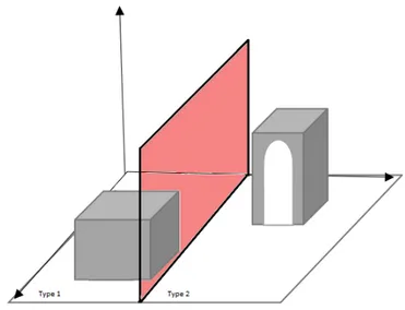
zones with different characteristics. The classification of the types of zone was introduced by Amigoni and Riva in [2] and by Ghiotti in [21]. They classified environments into two types:
• Type 1 comprises the environments in which an UAV covers a larger area when going up, this means that the area covered at given height is always included in the area covered at a higher height, as in an open field.
• Type 2 includes the environments in which the area that can be covered at given height is a subset of the area covered at any lower heights, as for an industrial area with sheds.
Type 1 zones are covered by a SingleHeight algorithm that produces paths over a fixed height amd selects the one with the minimum cost. Type 2 zones are covered by a TwoHeight algorithm that computes tours over two heights with a hierarchical approach, starting from the highest grid and going down, to cover incrementally the area left uncovered by tours at upper heights. Then it compares all the tours and selects the minimum-cost tour.
Every zone is covered separately as an independent environment. Firstly, a set of covering points is founded by the AGP using a greedy approach, then a TSP connects together the points, using Theta* to calculate the distance cost.
When all the zones are covered we merge the paths to produce a single path over the entire environment. A similar problem is faced by Galceran et al. in [19] where they used a divide-et-impera approach to cover the seafloor with an AUV (Autonomous Underwater Vehicle). We propose two different merge algorithms.
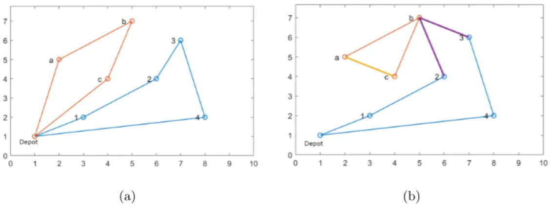
Merge Algorithm 1 selects one path as first and the other path as second. The edge that merges the two paths together links the last point of the first path to the first point of the second path.
Merge Algorithm 2 selects one path as external and the other as internal. All the points of the two paths are analyzed in a greedy way and the solution with the minimum distance cost will be selected. Calling (p1, p2) the points selected for the merge, we will have a final path that goes through the external path until
p1 is reached. Then goes to p2 and goes through all the internal path and returns to the external, returning to the depot.
We implement both algorithms on three different environments with different UAV sensor’s FOVs. We compare the results obtained with our divide-et-impera approach with the results obtained with a single CPP over the entire target area. Merge Algorithm 1 produces results in less computational cost but with a high distance cost. On the other hand, Merge Algorithm 2 has an high computational cost but produces better results in terms of distance.
1.1
Structure of the Thesis
The thesis is structured as follows:
• Chapter 2 discusses the state of art of CPP. More specifically: firstly, it introduces various coverage methods for 2D environments and then works about 3D CPP and multi-robot CPP are discussed.
• Chapter 3 introduces the problem studied in this thesis. We start describing the problem statement, how the environment is represented and the char-acteristics of the UAV. We analyse different types of environments and how a solution is obtained with our divide-et-impera approach.
• Chapter 4 outlines the divide-et-impera process in all its steps. How the division is done, the AGP algorithm and the TSP algorithm used. Then two merge algorithms are described.
• Chapter 5 introduces the simulation environment and the experimental tools. Then we describe and comment the results obtained.
• Chapter 6 summarizes the obtained results and proposes some possible fu-ture improvements.
• Appendix A illustrates occupancy grid maps of the environments used to test the algorithms.
• Appendix B illustrates the maps with the optimal path using both the merge algorithm for every environment and FOV.
ning (CPP) and will try to compare them to this study. More precisely, the survey of the works is divided in 2D and 3D approaches.
2.1
Introduction to CPP
Coverage Path Planning (CPP) is the task of determining a path along a set of points to cover an area or a volume of interest while avoiding obstacles.
There is a large variety of CPP algorithms and many different classifications of these. The most important classification is the one that divides the algorithms between the ones that operate a 2D coverage and the others that offer a 3D one. In the middle of these two groups are those algorithms that are used to cover a 2D surface while moving in a 3D space. In this thesis we refer to this particular class of CPPs.
Another possible classification is between online and offline algorithms. The former, take real-time measurements, decisions are calculated and used during the execution of the algorithm, the latter, have a complete knowledge of the en-vironment a priori, before execution.
Algorithms can also be divided basing on the type of the trajectory between points, fixed a priori or computed. For example, fixed trajectory consider a fixed track like a spiral or a circle, while computed trajectory is demanded to an algorithm. Often, the fixed trajectory algorithms are also offline but this is not always the case (our approach is offline with a computed trajectory). Another classification is on the type of coverage they offer (uniform or non-uniform). In non-uniform coverage some areas of the target area are skipped because not relevant, while this do not happen in uniform coverage. CPP is done by a single robot or by two ore more, in this case we talk about a swarm of robots that interact between them to reach a common goal.
(a) (b) (c)
Figure 2.1: (a)Example of trapezoidal decomposition [10]. (b) The boustrophedon decom-position [10]. (c) A path using boustrophedon decomdecom-position [10].
Environments can be modelled in different ways: polygonal as [10], grid-discretized as in [44], graph-based as in [42]. In particular, 2D model can be planar surface in the case of a floor cleaning, lawn moving, land mine detection, etc. In real scenarios, CPP is often done over 3D environments, for example in the case of UAVs covering fields, AUVs (Autonomous Underwater Vehicle) covering seabeds, or robots which are used to inspect the surface of objects like caves or build-ings. Sometimes 3D environments can be simplified using 2D planar surfaces at different heights like in [26] and in our thesis.
2.2
2D Coverage
Concerning 2D scenarios, Choset and Pignon [10] proposed an off-line, fixed tra-jectory approach: the boustrophedon cellular decomposition. It is an extension of the simplest cellular decomposition: the trapezoidal approach, in which the free space in the environment is divided in cells of trapezoidal shape. A drawback of the trapezoidal approach is that it generates many cells that can be merged to form bigger cells as shown in Figure 2.1(a). The boustrophedon cellular decomposition resolves this problem. Indeed, the free space is decomposed in non-overlapping regions, called cells, formed extending a vertical line both up and down from a vertex and choosing only the ones in which the line does not touch an obstacle in both the directions as shown in Figure 2.1(b). Then an adjacency graph between the cells is computed and, in each cell, a coverage path is found by means of back-and-forth motions. Finally, a path from one cell to another through the adjacency graph is reckoned as shown in Figure 2.1(c). This approach works only with polygonal obstacles.
In [1] the authors starting from the boustrophedon cellular decomposition proposed an evolution based on critical points of a Morse function, i.e., a Morse function is one that has non-degenerate critical points. A critical point is a point
(a) (b) (c)
Figure 2.2: (a) Cell determination using the Morse based decomposition [1]. (b) and (c) Morse cellular decomposition for h(x) = x2
1+ x22 in which the slices are circles. Rather than
moving along circular paths and stepping outward, the robot follows a spiral pattern [1].
ρ ∈ <m and exists a function h : <m → < that has all its partial derivatives are 0. The point ρ is non-degenerate if and only if its Hessian is not singular. Considering a single variable function, a critical point corresponds to local max-imum, local minmax-imum, or an inflection, while non-degenerate critical points mean points that are a maximum in some directions and a minimum in others. The authors defined a slice as a “pre-image of a real-valued function”, taking cue from Canny [8] method in which a slice is a codimension one manifold. While boustrophedon method extends cell lines from the vertices of the obstacles, the Morse decomposition traces the cell boundaries where a connectivity changes of the slice occurs in the free space. This fact occurs at critical points of the Morse function in correspondence of obstacle boundaries. Different cell shapes and dif-ferent coverage path patterns can be obtained choosing difdif-ferent Morse functions, as shown in Figure 2.2(b) and Figure 2.2(c). After the cell decomposition phase, a path in the adjacency graph is computed and a coverage path in each cell is generated.
While these two methods divide the environment in cells of different shapes, there are also methods that rely on a grid based decomposition, where each cell is equal to another one. This is also the method that we use for our thesis.
Zelinsky [44] presented an off-line grid based coverage method extending the distance transform path planning method proposed by [27], used to find a path from a start to a goal. The planner propagates a wavefront from the goal cell to the starting cell through all free space and around obstacles. A value is assigned to each cell, starting from the goal with 0 and giving 1 to all the neighbours (a neighbour cell is a cell directly linked, in the eight directions, to the one con-sidered) of the goal, and 2 to all the neighbours of the cells marked with 1 and so
(a)
Figure 2.3: An example of wavefront path [44].
on until the initial cell is reached. Then, from the starting cell a coverage path can be found choosing every time the highest unvisited neighbouring cell until the goal is reached as shown in Figure 2.3(a).
Gabriely and Ramon [18] proposed the Spiral STC (Spanning Tree Coverage) algorithm, an online approach with a fixed shape of the path as a spiral. The algorithm incrementally subdivides the environment in a grid of 2D-size cells, each one divided in four smaller cells of D-size as represented in Figure 2.4(a). Starting from the current cell, the robot selects the new 2D-cell to visit in anti-clockwise direction and adds it to the spanning tree as new edge. This process is repeated until no new neighbours are discovered. This coincides with the fact that the robot has reached the end of one side of the spanning tree. At this point it turns around and traverses the other side of the tree returning to the starting point. An example of the path computed by Spiral STC algorithm is shown in Figure 2.4(b).
Another approach based on 2D grid representation is the one proposed by Riva and Amigoni in [35]. They propose a CPP based on a Greedy Randomized Adaptive Search Procedure (GRASP). The GRASP was first introduced by Feo
(a) (b)
Figure 2.4: (a) (b) A solution using Spiral STC algorithm [18].
and Resende in [17], and it is a methauristic approach in which each iteration is composed of two phases: construction and local search. The construction builds a feasible solution, and then the local search tries to improve it. The GRASP method for CPP proposed by Amigoni and Riva first calculates an initial cover-age tour Sinitbased on a greedy approach. The greedy approach, at each iteration, randomly selects a vertex from the set of best vertices that can be reached from the current node, ordered according to a combination of distance and expected covered area. The local search procedure consists of two consecutive phases: ex-change and removal. During an exex-change a vertex in Sinit is substituted with a vertex not in the tour. At the end, when all the possible substitutions have been calculated, the substitution Sl1that produces the maximum decreases of the tour cost is selected. Then, removal excludes one vertex at once from Sl1, and if the solution is still feasible computes the new tour. Again, among all the new feasible solutions found by removal, the one with the maximum decreases of tour cost is selected. In such a way a local optimum is reached.
Tomoioka et al. in [39] propose an offline grid-based CPP method for mobile surveillance. Their method is based on MILP (Mixed Integer Linear Program-ming). First they decompose the target area in a grid, then a graph that considers the possible routes, on the basis of the camera orientation, is constructed. The tour is computed over it solving a MILP problem with the objective of minimizing the total travel time of the tour. To guarantee the optimum and find a feasible tour some constraints must be formulated:
• any target cell is observed from at least one camera candidate,
• the incoming flow of each vertex is equal to the outgoing flow to guaran-tee closed routes. (The flow f (e) is a non-negative integer variable that
represents the number of times the generated route passes through edge e), • travelling route constraints for the TSP formulation.
To reduce the solution space without losing any optimal solution, the authors propose to cluster groups of free cells in large problem instances.
Recently, advanced algorithms based on a two-step optimization process have been presented. In the first phase an AGP (Art Gallery Problem) is solved, which corresponds to find the minimal set of viewpoints (called guards or cov-ering points) that cover the whole free space (see Lee and LIn in [28]). In the second phase Travelling Salesman Problem (TSP), firstly introduced by Dantzig, Fulkerson, and Johnson in [14], is solved, which consists in computing the shortest tour to connect the points selected by the AGP.
(a)
(b)
Figure 2.5: (a) Optimal tour when travelling time is minimized first [3]. (b) Optimal tour when sensing time is minimized first [3].
Arain et al. [3] propose different offline grid-based algorithms to solve a prob-lem of sensor placement for gas detection. The authors limit the movement of the robot whit a finite set of poses pi = (αi, θi), where αi is a free cell of the space and θi is an allowed orientation. To compute the shortest path, the authors build a movement graph, to represent the possible movements of the robot in each cell
formulate it as a combination of a Watchman Route Problem (WRP) and an AGP. But, this formulation becomes practically unfeasible as the number of covering points grows, because both the WRP and AGP are NP-hard.
So, they consider two variations of a two-step approach:
• In one case, first selects the tour, with the minimum travelling time, that cover all the target area. And then picks the minimum set of covering points among the points of the chosen tour. This process is shown in Figure 2.5(a). • The other approach first finds the minimum set of covering points, and then
uses the TSP to compute the shortest tour as in Figure 2.5(b).
In both cases the problem has a bottleneck in finding the set of minimum covering points solving the following integer linear programming problem:
minimize CTTs subject to V C ≥ 1
C ∈ {0, 1}
Let CP be the set of candidate sensing configuration, Ts is a column vector of size |CP| that represents the sensing cost associated to each covering points, V is a binary matrix of size n × |CP|, where n is the number of cells in the problem. V [α, c] is equal to 1 if α ∈ vp(c), 0 otherwise. And C is a column vector of cardin-ality |CP|, whose elements are binary variables representing if a given candidate sensing configuration is selected or not. The main contribution of their work is to propose the conv-SPP algorithm, a variation of the previous integer linear pro-gramming problem to quickly finding the minimum set of covering points. It is based on a convex relaxation which introduces sparsity, so it drastically reduces the number of variables. Furthermore, it generates results very close to the op-timal ones.
Table 2.1 summarizes all the methods presented, with the most important characteristics in the foreground.
Reference Algorithm Offline/Online Trajectory
[10] Boustrophedon cellular decomposition
Adiacency graph Offline
Fixed
(back-and-forth motion) [1] Morse-based decomposition
Adiacency graph Offline
Computed
(depends on the cell shape) [44] Grid based decomposition
Wavefront Offline Computed
[18] Grid based decomposition
Spanning Tree Coverage Online
Fixed (spiral) [35] Grid based decomposition
GRASP (greedy + local search) Offline Computed
[39] Grid based decomposition
MILP solution Offline Computed
[3] Grid based decomposition
AGP + TSP Offline Computed
Table 2.1: Summary of 2D works presented.
2.3
3D Coverage
In the last years more and more UAVs are used in the CPP subject. In these cases the environment is no more a 2D one, but it’s a 3D dimension space, in which the robots can move not only in a plane but they can move in a space. In these environments 3D CPP is required, therefore the previous methods cannot be applied straightforwardly. In the field of 3D CPP the concept of 3D structural inspection is relevant in which it is necessary to cover 3D-surfaces as boundaries of buildings, ocean floors, agricultural fields, or automotive parts.
In [26] Hert et al. used a 2D planar algorithm to solve 3D CPP. They propose an on-line approach for an AUV to cover an unknown underwater environment. This approach consists in applying a 2D planar algorithm in the successive hori-zontal planes laying at different depths. In essence this means that the 3D sur-face is divided in successive planes at different depths and the intersection points between the planes and the 3D surface that must be covered, are projected onto the 2D plane. Robot adjusts its height so as to maintain a constant distance from the ocean floor. A constraint on the environment is formulated as any vertical line passing through the surface intersects it at exactly one point. Consequently there is a one-one correspondence between the points in surface and those in the x-y
(a)
(b) (c)
Figure 2.6: (a) The robot will cover area A with boundary B [26]. (b) At the top is shown a cross section in the plane y = y0, P1, P2 and P3 are points where the surface exceed the
threshold slope µ. In the bottom the area A is projected onto the 2D plane [26]. (c) Shows the path of the robot starting from SP [26].
plane and some elements as canvas cannot be present in this type of environment. This kind of non planar surface are called vertically projectively planar surfaces. This process is shown in Figure 2.1(a) and Figure 2.1(b). The considered 3D surface is bounded between two threshold surfaces, z = zmin and z = zmax. Each plane is represented using a semi-approximate cellular decomposition, in which the space is divided in vertical slices of the same width. The planar environment is covered zigzagging along parallel straight lines and starting from any point in the space as shown in Figure 2.6(c). In the projectively planar 3D environment the same zigzagging motion leads the robot from one grid plane to the next. The only addition is a vertical movement to pass from one grid to another to take into account the changes in the height of the terrain.
In our algorithm the 3D space, is divided in successive planes, but the planes are represented as equivalent grids at different heights with different occupancy
(a) (b)
Figure 2.7: Hemispherical simplification of urban structure and hemispherical trajectory of UAV [9]
values. This removes the restriction of a vertically projectively planar surface and does not impose a zigzagging behavior.
Another approach with fixed trajectory is proposed by Cheng et al. [9]. The authors propose an offline coverage algorithm for urban structures, the buildings with geometric solids such as cylinders and hemispheres. This simplification allows the authors to consider the problem as a problem of covering regular non-planar surfaces, as shown in Figure 2.7(a). In the hemispherical model the structures are approximated with a coverage hemisphere HC(OC, rC). Also the UAV trajectory is fixed, since it has to follow a flight hemisphere HF(OC, rF) where the center OC coincides with the center of the coverage hemisphere, while it holds that rF > rC meaning that the flight hemisphere is bigger than the coverage one. Intuitively, the UAV is moving along a sequence of horizontal circles at different altitudes to cover the area as shown in Figure 2.7(b). Similarly to our work they consider an UAV with conical FOV (Field Of View).
Bircher et al. [6] propose a two-step offline optimization algorithm to solve a structural inspection problem, a sub-problem of CPP which consists in finding a path that covers the whole surface of a desired structure. In this paper the 3D structure is represented by triangular meshes. The first step consists in selecting the viewpoints without following an optimization strategy, but trying to make the connecting path as short as possible. The idea behind this is that sometimes, due to a continuous sensing device, it is more important the position in the space of the viewpoints than their number. So, the authors only select a feasible view point for each triangle.
(a) (b)
Figure 2.8: Sampling scheme and its dual scheme proposed by Latombe and Gonzalez-Banos to solve a variation of the AGP [23].
of the AGP based on random sampling and introduced the first time by Latombe and Gonzalez-Banos in [22] and [23] has been used. Latombe and Gonzalez-Banos propose two approximations to solve the AGP as set covering problems for sensor placement to reconstruct a 3D image. They solve this problem assuming that a 2D layout of an horizontal cross-section of the environment is given.
The first algorithm samples the workspace W at random to have a set of guards candidates, G, and selects the subset with minimum cardinality. Then a greedy algorithm is applied to choose at each step the guard with the highest coverage of the uncovered boundary. First, let X be the set of the elements that must be covered, R = {R1, R2, ..., RM}, where Ri is the set of elements of X covered by element gi ∈ G, this is shown in Figure 2.8(a). The set Ri with highest cardinality is selected and removed from R and the elements of Ri are removed from X and from the other Rj ∈ R, with j 6= i. The process is repeated until X is empty. The second algorithm is based on a dual sampling scheme, shown in Figure 2.8(b). In the basic version of the random sampling algorithm, the complexity grows w.r.t. the number of samples. Instead, in the dual algorithm, the elements that must be covered are sampled, to have the possibility to vary the number of guards. So this time a point is selected from the unseen portion of the perimeter and the region from which such a point is visible, O(p), is computed. Then O(p) is sampled to find the position with highest coverage and a new guard is selected. The process is repeated until the unseen boundary is small enough.
The AGP based on random sampling and reduced to the set cover problem explained before, is called Coverage Sampling Problem (CSP) by Englot and Hover [16]. They define the CSP as the problem of finding a feasible covering set. The watchman route algorithm using dual sampling proposed by Danner and Kavraki [13] and the reduntant roadmap algorithm proposed by Englot an Hover in [15] are two examples of CSP. They use a range space representation of the
en-vironment, that consists in a set system (P, Q), where P is a finite set of geometric primitives of the structure that must be covered, and Q is the robot configuration space. These two algorithms and their stateflow diagram are illustrated in Figure 2.9, which is taken from [16].
Figure 2.9: Stateflow diagram illustrating two algorithms based on CSP [16].
The watchman route algorithm using dual sampling [13] consists of a first phase in which the variation of the AGP proposed by Latombe and Gonzalez-Banos [22], [23], is used. In the second phase a weighted graph is built. This graph consists of one node for each guard, and one edge for each pair of guards with weight equal to the length of the shortest collision free path between the two nodes. To find the shortest free path between two points, Probabilistic Roadmaps (PRM) are used and an approximation of the TSP is solved over PRM.
The redundant roadmap algorithm [15] solves the variation of the AGP by randomly sampling configurations until the required structure is covered. To rep-resent the required structure, the authors use a triangular mesh model obtained from real sonar data. The first phase lies in building a redundancy roadmap, that collects the robots configurations and catalogs their sensor observations, creating a discrete state space from which a inspection path will be built. In a redundancy roadmap, each point has to be covered a given number of times. So, the first phase consists in selecting a geometric primitive, that has not been covered the given number of times yet, and adding to the roadmap a random robot configuration in the neighborhood of the selected primitive.
(a) (b)
Figure 2.10: Path generated by the Cone-TSPN algorithm [33].
greedy algorithm that adds at each iteration the roadmap node with the largest set of observed primitives not yet in the cover. Then, the set covered is pruned with an iterative approach. At each iteration a configuration, that is not the unique observer of a geometric primitive, is randomly removed from the set cover until every configuration in the set is the unique observer of at least one primitive. Then, it is invoked a lazy TSP algorithm, the one proposed by Christofides [11], employing an iterate solution of the Rapidly-exploring Random Tree (RRT) over all goal-to-goal paths in the tour.
Another important study consists in the trade off between flight-time and cov-erage: Plonski and Isler [33] propose an offline approach based on a variation of Neighbourhoods-TSP (TSPN) called Cone-TSPN. In order to capture an image of a set of chosen points, the algorithm considers a set of inverted cones, each one with the vertex in one of the chosen points, with slope Π/2 − α and a given height h ∈ H.
The aim is to find a minimal tour that intersects all the cones. Due to the fact that this problem is NP-hard, the authors find the tour that better approximates the length of the optimal tour. Let be bh the max estimated height, defined as b
h/2 ≤ h∗ ≤ bh, where h∗ is the maximum height obtained by the optimal tour. They compare the cost of a tour on cones at the same height with the one of the tour on cones at different heights. The analysis is different for disjoint cones and for non-disjoint cones. For disjoint cones at same height a SLICE-VISIT strategy is proposed. It consists in truncating all cones higher than the bh, in-tersecting all the cones with a plane at height ht, where ht = min(H), and finding the TSPN tour that visits all the circular cross sections of the cones in this plane returning to the starting point at height 0. Considering different heights SLICE-VISIT cannot move higher than min(H) so the authors classi-fied the cones according to their height performing SLICE-VISIT for each class of
(a) (b) (c)
Figure 2.11: (a) Workplace identification [41]. (b)Coverage trajectory generated [41]. (c) Mosaic reconstruction [41].
cones, in practice they consider multiple planes. The authors obtain an approxim-ation factors of the length of tour that is independent from the number of cones in both cases: for single height O(( max(H)
mean(H))
2(1 + tan(α))) and for multiple heights
O((1 + logmax(H)
min(H))(1 + tan(α))). So the tour at different heights computes tours shorter than the one at the same height. Authors extend this analyses also for non-disjoint cones. Notice that, differently from us, Plonski and Isler select points of interest a priori. Also, their problem is formulated within an Euclidean plane without obstacles.
Valente et al. in [41] apply the problem of coverage to the precision agriculture. The authors first decompose the environment, using a grid-based representation with optimal dispersion dividing the space in cubes. Then the grid is converted in a graph and the coverage path is computed selecting from the start point the nearest neighbor cell in gradient order. When more neighbors are present, a cost function is used to select the best one. Using a depth-limited search a tree of all the possible coverage paths is built in order to select the one that passes thorough all the nodes only once. The computed path is shown in Figure 2.11(b).
Nam et al. in [31] describe an offline approach for UAVs CPP in a survey mis-sion. The method adopted by the authors uses a grid-based decomposition and a wavefront algorithm. The terrain that must be covered is divided in rectangles like in Figure 2.12(a) (start position is represented by the rectangle in blue, the green one is the goal that must be reached from the robot). It is assumed that the Field Of View of the robot can sense all the rectangle’s area from the centre of it. After this a wavefront algorithm provides all the solutions from start to the goal point avoiding obstacles and the one with the best cost is selected as solution (Figure 2.12(b)). To improve the final result they implemented also a cubic spline
(a) (b) (c)
Figure 2.12: (a) Grid-based decomposition [31]. (b)Optimal path generated by wavefront algorithm [31]. (c) Coverage trajectory generated by cubic interpolation [31].
algorithm to smooth the path cutting away the angles as in Figure 2.12(c). Galceran et al. in [19] propose an offline method for covering complex struc-tures over the ocean floors using an AUV. The idea is to use a 2.5-dimensional (2.5D) bathymetric map of the floor to distinguish the planar area in the target zone and the high slopes that represent the 3D objects. Two different algorithms are then used to cover these two types of zones, producing different paths. Regard-ing the 2D planar surface, CPP is done by dividRegard-ing the area with boustrophedon decomposition and a simple mowing-the-lawn motion producing a path similar to the one in Figure 2.13(a). For the 3D high slopes the bathymetric map is intersected with slice planes and an AUV contours the slopes maintaining a fixed offset from the target surface as we can see in Figure 2.13(b). These two distinct paths must be merged into one final path that covers the entire seabed as we can see in the tree in Figure 2.13(c). The problem to merge differents paths is not specifically addressed in the article, but is important as in our thesis we also have different paths to be merged into one.
Recently, Amigoni and Riva in [2] proposed an offline 3D CPP to cover a 2D surface using an UAV. The problem faced is to cover a field in the least possible time with a robot that starts in a fixed point and return to this. They discretized the environment in different 2D planar surface at different heights each one rep-resented by a grid-based map. The solution adopted is a two-step approach that combines AGP to select the minimal number of points to cover the target surface and TSP that search the optimal path that passes through all the points selected
(a) (b) (c)
Figure 2.13: (a) Coverage path of the planar region [19]. (b)Coverage path planning of the high slopes [19]. (c) Diagram of the coverage path-planning algorithm for bathymetric maps. [19].
in precedence. In the next chapter this work is studied more as its the starting point for our thesis.
There are CPP works that propose also a non uniform type of coverage. These algorithms do not cover the entire target surface but they skip some area because, for some criteria (can be various and depend on the purpose of the CPP), are not important towards the goal of the CPP. Because of this the final coverage path goes only through some zones, reducing the target surface. This approach saves resources and minimizes the total cost.
Sadat et al. in [36] propose an online non uniform algorithm for CPP of a field. It can be used in a vast variety of applications such as agriculture, surveillance, search and rescue, and vegetation monitoring. The solution uses an UAV with a micro-camera whit a square FOV that has an higher resolution when its distance from the target surface is minimal. The method exploits the visit over a tree based on the Hilbert Space Filling Curve (SFC) to calculate a path minimizing the cost and exploiting the locality of the interesting regions. The tree is constructed in a way that the nodes within a depth represent a square in the map and a particular resolution (height from the target surface). Root represents the highest height while the leaves the height where the camera resolution is at its maximum. The authors use the Hilbert curve to impose an ordering on the nodes at each level of the coverage tree. The Hilbert curve is a fractal space-filling curve shown in Figure 2.14(a). Informally speaking if a robot follows a Hilbert trajectory, it is certain that it stays close to the recent places that it has visited. This means that when an interesting region is observed, one can opportunistically assume that the next node will also be interesting due to the locality preserving feature of the Hil-bert curve 2.14(b). The final algorithm starts visiting the root of the tree, every
(a)
(b)
Figure 2.14: (a) Hilbert curve with different orders [36]. (b) Coverage tree with hilbert-based ordering of nodes at each depth and its relationship to grids in different resolutions [36].
Lee et al. in [29] propose an online non uniform approach to cover the seafloor using an AUV with a FOV represented by a rectangular polyhedron. The 3D environment is simplified by 2D planes at different depths. The solution relies on the concept of Artificial Island (AI). An AI is an area in a plane in which there are no obstacles and boundaries. The algorithm works in a recursive way, it consecutively scans the entire area of a plane before moving up to the next plane. Now, defining η as the sensor reliability coefficient, zt as the measurement value, xt as the robot position at time t and m as the environment information and h as the length of the robot sensor, if the equation η ≤ p(zt≤ h2|xt, m) holds it means that a boundary or obstacle exists in the upper plane with respect to the current position. In the other case, when the equation does not hold it means that in the upper plane in the position where the perception is done in the lower plane, there is a safe area. Due to this, that area in the covering of the next plane can be skipped reducing the time end the cost of the final path.
Figure 2.15: Flowchart of the system proposed by Barrientos et al. [4].
the the most important characteristics.
2.4
Multi-UAV Coverage
Regarding the use of multiple robots for CPP, the literature highlights many pro-posals due to the advantages of extending the CPP from single robot to multiple robots as the decrease in time, improvements in robustness, and so on. There-fore many of the works discussed above were transformed and reformulated to multi-robot coverage like Rekleits et al. [34] who extend the boustrophedon de-composition to multiple robot scenarios imposing some rules to coordinate the robots.
Maza and Ollero [30] proposed a method for multi-robot CPP at constant height. Firstly the target area is decomposed in polygonal regions using sweep line approach, then each polygon is assigned to a different UAV taking in account the capabilities of each UAV, like flight endurance and range. Once each UAV has an area assigned, this is covered by a back and forth motion along rows per-pendicular to the sweep direction of the polygon so as to ensure the minimum number of turns in an area.
A multi-UAV approach at constant height is proposed by Barrientos et al. [4]. The aim of their work is to propose an efficient algorithm for precision agriculture using a multi-UAV system. Initially the target space is divided in different areas solving a task subdivision and allocation problem with two restrictions: each ro-bot knows its own characteristics and status but does not know anything about the other robots. They solve this problem as a negotiation process in which each robot tries to obtain as much area as possible, rather than assign a region to a robot using geometric considerations. Then the path to cover each waypoint
Reference Algorithm Offline Online T ra jectory [26 ] Multiple 2D p lanes at differen t heigh ts Semi-appro ximate cellular decomp osition Online Fixed (zigzag along parallel lines) [9 ] Geometric semplifi c ati on of target complex structures Offline Fixed (emisphere) [6 ] A GP+TSP Offline Computed [13 ] W atc hman route algorithm with dual sampling (v ariation of A GP base d on the idea of CSP + w eigh ted graph) Offline Computed [15 ] Redundan t roadmap algortihm (v ariation of A GP based on the idea of CSP + set co v er sub-problem + lazy-TSP) Offline Computed [33 ] Cone-TSPN at differen t heigh ts (v ariation of Neigh b ourho o ds-TSP) Offline Computed [41 ] Grid-based decomp osition in cub es Graph tree visit Offline Computed [31 ] Grid-based decomp osition W a v efron algorithm (rectangles) Cubic spline to smo oth the path Offline Computed [19 ] 2.5D bath ymetric map Merge of tw o differen t algorithms (b oustrophedon decomp osition for planar area, 3D coun tour for slop es) Offline Fixed (mo wing-the-la wn, circles for slop e s) [2 ] 2D planar su rfaces at differen t heigh ts A GP+TSP Offline Computed [36 ] Grid based Visit of a tree exploiting Hilb ert Space Filling Curv e Online Computed [29 ] 2D planar su rfaces at differen t heigh ts Co v ering consecutiv ely planes exploiting AIs Online Dep ends on co v erage algorithm used T able 2.2: Summa ry of 3D w o rks p re sented.
(each point of interest) has to be planned for each robot and it can be solved as a simple CPP: they have developed an extension of the wavefront planner previ-ously explained. A scheme of this process is shown in Figure 2.15.
The two previous papers consider only one height of flight for UAVs, while Basilico and Carpin [5] propose a multi-UAV CPP on two levels for surveillance. They consider heterogeneous UAVs and divide them in sentinels and searchers, where sentinels are positioned at higher heights and are tasked to control large areas and detect some type of events called attacks. Searchers depend on sen-tinels, since they fly at lower heights and detect with less errors an attack when notified by the sentinels. The authors model the environment as a grid of equally sized squared cells and the presence of an attack in a cell c as a loss value l(c). They define a binary function a(c, t) that indicates if a cell c is attacked at time t. Their goal is to minimize the overall loss computed as P
c∈Gl(c) RT
0 a(c, t)dt, where G is the search domain, and T is a finite time horizon. Their aim is to cover all the area at risk, so if a zone is safe, no UAV will cover it.
Finally Table 2.3 reports all the multi-robot CPP methods analyzed in this section.
Reference Algorithm Online
Offline Trajectory
[34] Extension of 2D boustrophedon decomposition
to multiple robots Offline Fixed
[30] Polygonal regions decomposition
(each polygon assigned to a root) Offline
Fixed (back and forth)
[4] Division into sub regions
(negotiation between robots to obtain the most wide area) Offline
Depends on the CPP used [5]
2 levels division
UAVs on the upper level cover large areas UAVs on the lower level cover little areas
Offline Computed
work done by Amigoni and Riva in [2] and by Greta Ghiotti in [21] since it is the starting point for our considerations. Then, we introduce our idea to improve the results obtained in these two works.
3.1
Problem Statement
In [2] the authors presented the coverage path planning of a robot that moves in a 3D space and that must cover a 2D target surface (a field for example).
They considered a single robot that can move in a three-dimensional environment as an Unmanned Aerial Vehicle (UAV) starting from a fixed cell (called depot) and returning to the same depot. The robot has to compute a tour such that the ground of the environment is completely covered by the robot’s sensor at the minimum cost (either time or distance travelled).
The environment is discretized by 2D planes at different heights and each plane is modelled as a grid of identical cells with a square shape. We can see this model in the Figure 3.1(a).
Each cell is defined by a set of coordinates (x, y, z) where x,y denote position in the plane, while z denotes the height in space. Each cell can be free if the UAV can move in it or occupied if there is an obstacle that prevents movement. The depot is always on the ground and is defined by (x, y, 0).
The UAV has a sensor with a conic Field Of View (FOV) that projects to the ground a circle with a radius equal to r = h · tan(α), where h is the height of cone and α is half of the apex angle (Figure 3.1(b)). It is assumed that each perception P (f ) (where f is a free cell) is constant and is equal for any f ∈ F for every height.
(a)
(b)
Figure 3.1: (a) Example of 3D decomposition in different planes [2]. (b) Example of the FOV varying with height [2].
The goal of the CPP presented was to find a path that covers all the ground cells that is,
[
1<i<k
C(fi) = F (0).
where C(fi) represent all the area covered at the ground from the cell fi, F (0) is the set of free cells at the ground and k is the length of a generic path. The cost
They classified the environments in two possible types:
1. type 1: an open field (like an agricultural one), where the coverage function is monotone with respect to the height. In this type of environment the UAV will cover more area when going up. This is true when it holds the following equation,
C(f ) ⊆ C(f0), 0 ≤ h < h0≤ Hmax.
where C(f ) and C(f0) are respectively the coverage function at f = (x, y, h) and f0 = (x, y, h0). An example of this environment can be seen in Figure 3.2(a).
2. type 2: a field where there are open building (like caves). In this case the area that can be covered at a given height is a subset of the area covered at any lower height,
[
f ∈F (h0)
C(f ) ⊆ [ f ∈F (h)
C(f ), 0 ≤ h < h0 ≤ Hmax.
Figure 3.2(b) shows an example of this environment.
In environments of type 1 they demonstrated that the space of the solutions can be reduced to only tours over a single fixed height without worsening too much the optimal solution. Results in this case showed that the optimal tours in terms of path length are at the highest height with a little FOV apex angle because this will reduce the number of covering points. When the FOV apex angle gets bigger the best paths are in the middle heights because when the UAV has a very large FOV there is no advantage in going up due to the fact that after a certain height there is not a reduction in the number of covering points. Going at higher levels in these cases is only counterproductive because of the travel cost of going up.
In type 2 environments was invented a coverage tour over multiple heights. It is assumed that only the cells at height K can cover all the target cells at h0 because the openings in obstacles and buildings can occur only at height K (assuming that the openings are only at hmin 6= h0). The coverage algorithm cal-culates paths over the combinations of height K (fixed) and a level h ∈ (H \ h0)
(a) (b)
Figure 3.2: Examples of (a) Type 1 (b) Type 2
where H is the set of all the heights. Firstly an ArtGallery procedure finds the covering points at height h, then ArtGallery is called again at height K to cover the cells at the ground that can not be covered from height h. From height K is assumed that all the cells at the ground can be covered. Lastly, a TSP procedure is called to find a path between the covering points that minimizes the distance cost. In this case results showed that a path over a single height is never preferred over a path over 2-height because like in case 1 going up can reduce the number of the covering points, reducing the total cost too.
Regarding computational cost the algorithms with the most significant impact are the AGP and TSP. Results showed that AGP time depends on the extension of the area to cover (larger is the area bigger is the time to compute AGP) while TSP depends on the number of covering points (T SPt= O(n)).
3.2
Problem Analysis
The problem that we face in this study is to obtain a better computational cost of the coverage algorithm presented in the previous section.
Our approach is a divide et impera process. In computer science a divide et impera approach consists in simplyfing the problem in two or more sub-problems that are more simple to resolve. After that, the solutions of the sub-problems must be combined together to produce the final result.
In our case, we divide the entire map into different 3D-zones producing different paths that must be merged into one unique path to obtain the coverage path of
equal to the entire map,
xi∩ xj = 0, xi∪ xj = X ∀j 6= i
where X is the entire 3D map and xi and i = 1, ..., n represents the 3D-zones in which is divided X.
The division of the map is done such that a 3D-zone have the characteristics of only one environment (type 1 or type 2) and is not a mixed type environment. By doing this, we can cover the ground with SingleHeight algorithm if the portion of the map is type 1, or TwoHeight algorithm if the portion of the map has the characteristics of type 2 maps. In Figure 3.3 we can see a simple environment division into two distinct 3D-zones of different types. In the end we will have a path (starting from a common depot and returning to it) for every 3D-zone in which the entire map is divided.
Figure 3.3: Division of the entire map in two 3D-zones. On the left a type 1 environment, on the right a type 2 one.
cost. The resulting path will have the same depot of the paths merged and a number of covering points equal to the sum of covering points of the two paths excluding the depot for one of them. A similar process is done in [19] and is described in the previous chapter.
Using this divide et impera approach, we have a reduction in terms of com-putational time because AGP has to work on a little portion of the target area, and the number of covering points obtained with AGP is limited, especially with larger FOVs, helping TSP to obtain a path in less time with respect to obtaining a path over the entire environment.
To this possible reduction of computational time corresponds a possible worsen-ing in the distance cost because the TSPs over the zones are optimal only over the area covered. In fact merging paths that have TSP local optimality over a 3D-zone does not produce an optimal path over the entire area.
we present the methods that are used to calculate the covering paths in the 2 different types of environments introduced in Chapter 3. Then we describe two different merging algorithms.
4.1
First step process methods
In this section we analyse the methods used to find the covering points through AGP and the ones used to produce a path with TSP.
4.1.1 Art Gallery Problem
The AGP is the very first step of our entire process. AGP represent a visibil-ity problem born from a real-world problem of guarding an art gallery with the minimum number of guards. From this, AGP was studied a lot during the years and is defined as a minimum number of guards in a environment, which together can view the whole environment. This problem is NP-hard also in simple envir-onments.
We solve the AGP as a set cover problem, so our aim is to find the smallest possible number of cells, called S, that together can cover all the target cells on the ground F (0) (in our case F0 represent the ground of the zone on which the AGP is called). The set cover problem is again a NP-hard problem, but in [38] the authors demonstrated that the number of covering points found by general greedy approaches is, at most, OP T · log|F (0)|, where OP T is the number of covering points of the optimal solution of the AGP.
We propose a greedy algorithm, choosing at each iteration the guards with the highest number of cells covered among the remaining uncovered target cells at the
ground (h0). When more than one guards cover the same number of cells, one is selected randomly. After a covering point is selected, it is removed from the set of possible covering points and the covered cells are removed from the target cells. Therefore, the next covering point is selected from those that cover the remaining uncovered cells. The algorithm finishes when all the target cells are covered. AGP is described in Algorithm 1. Function ArtGallery(h, F(0)) is while isempty(F(0)) do s =arg max(CoverageArea(h, F(0))) S.Insert(s) F(0) = F(0) \ C(s) end return S end Function CoverageArea(h, F(0)) is
return the number of cells at the ground of the 3D-zone covered by each cell at height h in the environment
end
Algorithm 1: Art Gallery function
In the AGP algorithm, the CoverageArea function will return the candidate covering cells for our paths. In our case, the candidate covering cells are selected among the cells within the borders of the 3D-zone on which the AGP is called. To obtain the set of these cells we manually set the boundaries of the 3D-zone that we are considering and a simple algorithm selects all the cells in these borders. In our solution, we must produce a set of covering points through AGP for every 3D-zone in which is divided the entire environment.
4.1.2 A* and Theta* algorithms
We use Theta* search algorithm to compute the distances between covering points before applying the TSP and after to obtain the complete path between the cov-ering points. Since Theta* is based on A* algorithm we quickly introduce this before speaking of Theta*.
A* algorithm
The A* algorithm [25] is an extension of Dijkstra algorithm. A* uses a heuristic function h(s) to choose a neighbour vertex without exploring all the neighbour vertices. This heuristic function is an estimation of the cost from the current vertex s to the goal. A* maintains two values for every vertex: the g-value g(s)
Figure 4.1: A* grid path versus true shortest path [12].
that is the length of the shortest path from the start to the current vertex, and the parent value parent(s). A* uses two sets: open and closed to evaluate the vertices.
• The open set is a priority queue (based on the g-value g(s) of every vertex plus the heuristic function h(s), g(s) = g(s) + h(s)), that contains the discovered vertices that are not evaluated yet.
• The closed list is the set of vertices already evaluated.
A* uses the U pdateV ertex(s, s0) function to update the g and parent values of an unexpanded visible neighbor s0 of s using the procedure ComputeCost(s, s0). ComputeCost updates the g and parent values only if the sum between the ac-tual distance from the start to the current vertex g(s) and the cost of the path in straight line between s and s0, c(s, s0), is lower than the actual distance between s0 and start, g(s0). When the goal is reached, the algorithm ends. The procedure is reported in Algorithm ??.
If h(s) is admissible (it never overestimates the cost of reaching the goal) and consistent (its estimate is always less than or equal to the estimated distance from any neighboring vertex to the goal, plus the cost of reaching that neighbor.), A* guarantees to find the shortest path on a graph restricted to the grid shape, but this shortest path does not correspond to the shortest path in the continuous environment as shown in Figure 4.1. For this reason Theta* algorithm was de-veloped firstly in [12] and used today in many covering problems like ours.
Theta* algorithm
Theta* and A* is in the ComputeCost function where two possible paths can be found: Path 1 as before is the path in straight line, instead, Path 2 considers also the path from the start vertex to parent(s) and from parent(s) to s0, if s0 has line-of-sight to parent(s). This allows the parent of a vertex to be any vertex. Again the g and parent value of s0 are updated only if the sum of the g(parent(s)) and c(parent(s), s0) is lower than the shortest path from the start vertex to s0 found so far. The new pseudocode of ComputeCost function is described in Algorithm 2.
Function ComputeCost (s, s0)is if LineOfSight(parent(s),s’) then
// Path 2
if g(parent(s)) + c(parent(s), s0) < g(s0) then parent(s0)=parent(s) g(s’)= g(parent(s)) + c(parent(s),s0) end else // Path 1 if g(s) + c(s, s0) < g(s0) then parent(s0) = s g(s0) = g(s) + c(s, s0) end end end
Algorithm 2: Pseudocode for Theta* algorithm [12]. Distances with Theta*
In our problem Theta* is used not only to calculate the final path between all the covering points but also to calculate the matrix distances that is used by TSP to find the optimal order of visit. To do this, a variation of Theta* is used. The goal is removed and the algorithm is iterated for each coverage point returned by AGP. Substituting at each iteration the starting vertex with the current cover-age point we calculate the g-value that corresponds to the distance between the pair of points considered. When all the points are visited the distance matrix is generated and passed to the TSP.
It was formulated as an integer program for the first time by Dantzig, Fulker-son, and Johnson [14]. In our coverage problem we follow their formulation. Once the AGP has returned the selected points S, we want to minimize the trav-elling distance between them.
Before applying TSP, we transform the 3D environment in a weighted graph G, where the vertex of G are the cells of the environment and the edges have a weight equal to the distance dij between each pair of vertex i and j of G. dij is calculated using Theta* (explained in Section 4.1.2).
Let V be the set of vertices of the graph G. Then the total travelled distance is the sum of the distances of the vertices in the tour:
travelledDistance = X (i,j)∈V
di,jxi,j.
Where xi,j is a binary variable, that is 1 if cell(i, j) ∈ tour, 0 otherwise. The tour should pass only once through each vertex:
X
j∈V
xi,j = 2,∀i ∈ V.
Therefore for every vertex i exactly two of the associated xi,j variables should be equal to 1 so that the condition above is true, meaning that a vertex xi can appear only one time in a path (one, when from a generic cell we go to the cell xi and two, when from xi we go to another cell). At this moment we can produce solutions that are not connected tour, finding subtours. So we add a constraint to eliminate subtours, requiring that for each nonempty subset Sub of the set of covering points V , the number of edges between the vertices of Sub must be at most |Sub| − 1, so:
X
i,j∈V,i6=j
So finally the integer program becomes: minimize X (i,j)∈E di,jxi,j subject to X j∈V xi,j = 2 ∀i ∈ V X i,j∈Sub,i6=j
xi,j ≤ |Sub| − 1, ∀Sub ⊂ V, Sub 6= 0 xi,j ∈ {0, 1}
This is only one of the possible methods that can be used to produce a solution to a TSP problem, in literature there lot more of this for example Neighbourhoods-TSP (Neighbourhoods-TSPN) described in Chapter 2.
4.2
The Coverage Algorithms
In this section we describe how the two-phase method previously proposed is applied to the environments of Case 1 and Case 2 presented in Chapter 3. Type 1 comprises all the environments with a monotone behavior, as the case of covering a field. Basically we cannot have an obstacle at height h if this obstacle is not present at height h0< h.
Instead, Type 2 includes the environments in which the area that can be covered at a given height is a subset of the area covered at any lower heights.
We decided to formulate two different algorithms for the two cases: • SingleHeight algorithm for Type 1,
• MultiHeights algorithm for Type 2. 4.2.1 SingleHeight Algorithm
SingleHeight Algorithm is used to cover environments of Type 1 described in Chapter 3. As we have seen, to cover this type of area it is sufficient to generate a path over each 2D plane independently with AGP and TSP and then select the path with the minor distance cost. This is possible because we are sure that if we have not an obstacle at height h we are sure that an obstacle is not present at height h0 < h (with (x, y) = (x0, y0))
As shown in Algorithm 3, the SingleHeight algorithm considers each of the 2D grids at the different heights h ∈ (H \ h0). Firstly, the ArtGallery procedure is applied to every grid to find the covering points. Then T heta∗ is called to calculate the distances between each pair of covering points. Eventually, the TSP algorithm is applied |H| − 1 times every time using the covering points of the 2D
![Figure 2.9: Stateflow diagram illustrating two algorithms based on CSP [16].](https://thumb-eu.123doks.com/thumbv2/123dokorg/7524734.106380/32.918.182.713.304.581/figure-stateflow-diagram-illustrating-algorithms-based-csp.webp)
![Figure 2.15: Flowchart of the system proposed by Barrientos et al. [4].](https://thumb-eu.123doks.com/thumbv2/123dokorg/7524734.106380/38.918.193.733.191.365/figure-flowchart-proposed-barrientos-et-al.webp)