Behaviour of wooden structures with new seismic resisting walls : shaking table experimentation and its numerical simulation

(1)

Scuola di Architettura Urbanistica Ingegneria delle Costruzioni

Laurea Magistrale in Ingegneria dei Sistemi Edilizi 

Behaviour of Wooden Structures with New Seismic

Resisting Walls: Shaking Table Experimentation and

Its Numerical Simulation.

Supervisor: prof. Maria Adelaide Vittoria Parisi

Co-supervisor: prof Hiroshi Kawase

Thesis by:

(2)

(3)

Acknowledgements

I would like to mention those who helped me with this research, starting from professor Hiroshi Kawase from Kyoto University that has always been present during my time spent in Japan with his technical advice, his time and courteousness.

A special word of thanks to my Italian professor from Politecnico di Milano, Maria Adelaide Parisi, that helped me to check and complete my thesis work with her time and her professional knowledge and experience.

Another person that helped me to complete my research and make my time in the Japanese university more pleasant is my friend and lab mate Yagi Takachika.

I owe a special thank-you to my parents who allowed me to do this experience abroad, who have supported me every single day and never stopped believing in me.

A great thanks to my girlfriend Carlotta that encouraged and supported me in my long working trip and always sustains and helps me during the hard times, making me smile every day. I want also to thank my lifelong friends of my hometown, all of them know the sacrifice I did and they relieved me and made my life better.

In conclusion I want to mention my university mates, we helped each other during all this time, professionally growing every day, making me a better person.

(4)

(5)

Index

ACKNOWLEDGEMENTS 3

INTRODUCTION 20

1 THE STRUCTURE OF A TRADITIONAL JAPANESE HOUSE 25

2 JAPANESE SEISMIC DESIGN CODE 30

2.1 FIRST PHASE DESIGN FOR EARTHQUAKE ... 33

2.1.1 LOAD COMBINATIONS AND DESIGN METHOD ... 33

2.1.2 EVALUATION OF SEISMIC FORCE ... 34

2.1.3 THE SEISMIC ZONE FACTOR ... 35

2.1.4 THE VIBRATION CHARACTERISTICS FACTOR ... 36

2.1.5 STORY SHEAR FORCE DISTRIBUTION FACTOR ALONG BUILDING HEIGHT AI ... 38

2.1.6 STANDARD SHEAR COEFFICIENT ... 39

2.1.7 SEISMIC FORCE ACTING IN THE BASEMENT ... 40

2.2 BUILDINGS FOR WHICH THE SECOND PHASE DESIGN IS NOT REQUIRED ... 41

2.3 THE BUILDING STANDARD LAW OF JAPAN ENFORCEMENT ORDER ... 43

3 MODELLING AND ANALYSIS OF BUILDING TESTS 49 3.1 SAP2000 MODEL ... 54

3.2 MODAL ANALYSIS ... 62

3.3 NUMERICAL VERSUS EXPERIMENTAL RESULTS ... 64

3.3.1 DISPLACEMENT – SHEAR FORCE RESULTS ... 65

3.3.2 GENERAL COMPARISON ... 95

3.3.3 SPECTRAL RATIO RESULTS ... 101

4 MODELLING AND ANALYSIS OF REAL BUILDINGS 135 4.1 BUILDING 1 ... 136

4.2 BUILDING 3 ... 153

4.3 BUILDING 7 ... 170

5 CONCLUSIONS 187

(6)

Figures index

Introduction

-‐ Figure 1: Vertical plan of the WoC

-‐ Figure 2: Horizontal plan of the full-sized specimen with WoC: the plan on the top represents the second floor, the plan on the bottom represents the first floor

1. The structure of a traditional Japanese house

-‐ Figure 1.1: pit-dwelling house (realestate.co.jp) -‐ Figure 1.2: example of shinden-zukuri house -‐ Figure 1.3: house in Kyoto

-‐ Figure 1.4: traditional Japanese structure (cultorweb.com)

2. Japanese seismic design code

-‐ Figure 2.1: traditional Japan -‐ Figure 2.1.3.1: seismic zones -‐ Figure 2.1.4.1: values of TC

-‐ Figure 2.1.5.1: the vertical distribution factor Ai -‐ Figure 2.1.7.1: seismic coefficient for basement

3. Modelling and analysis of building tests

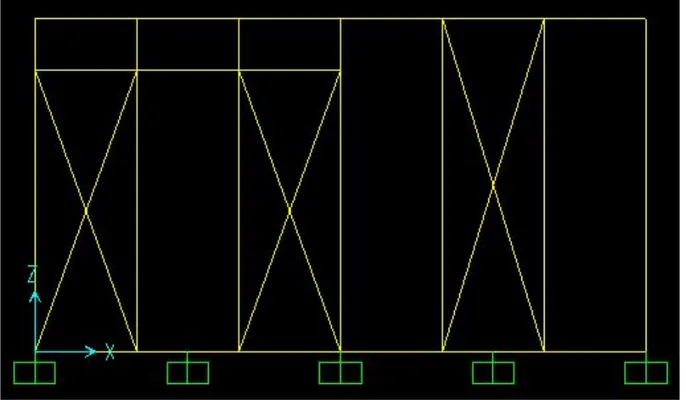
-‐ Figure 3.1: horizontal view of the tested building -‐ Figure 3.2: vertical view of the test’s building -‐ Figure 3.3: horizontal view, 8 wall of columns -‐ Figure 3.4: horizontal view, 4 wall of columns -‐ Figure 3.5: horizontal view, 2 wall of columns -‐ Figure 3.6: vertical view, final braces

(7)

-‐ Figure 3.1.4: vertical plan of the full-sized specimen with WoC, WoC side

-‐ Figure 3.1.5: vertical plan of the full-sized specimen with WoC, two-sided braces side -‐ Figure 3.1.6: vertical plan of the full-sized specimen with WoC

-‐ Figure 3.1.7: diaphragm constraint -‐ Figure 3.1.8: joint restraint

-‐ Figure 3.1.9: time history definition -‐ Figure 3.1.10: vertical loads

-‐ Figure 3.3.1.1.1: 8 Wall of columns, Kobe 10%. Numerical results

-‐ Figure 3.3.1.1.2: 8 Wall of columns, Kobe 10%. Comparison of numerical vs experimental results

-‐ Figure 3.3.1.1.9: Young modulus of Wall of columns -‐ Figure 3.3.1.1.10: Young modulus of Beams

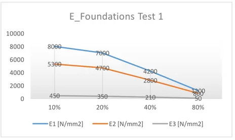
-‐ Figure 3.3.1.1.11: Young modulus of Braces -‐ Figure 3.3.1.1.12: Young modulus of Foundations

(8)

-‐ Figure 3.3.1.2.11: Young modulus of Braces -‐ Figure 3.3.1.2.12: Young modulus of Foundations

-‐ Figure 3.3.1.3.11: Young modulus of Braces -‐ Figure 3.3.1.3.11: Young modulus of Foundations -‐ Figure 3.3.2.1: Shear Modulus plot comparison, WoC -‐ Figure 3.3.2.2: Shear Modulus plot comparison, Beams -‐ Figure 3.3.4.3: Shear Modulus plot comparison, Braces -‐ Figure 3.3.2.4: Shear Modulus plot comparison, Foundations -‐ Figure 3.3.2.5: damping coefficient plot, test 1

-‐ Figure 3.3.2.6: damping coefficient plot, test 2 -‐ Figure 3.3.2.7: damping coefficient plot, test 3

(9)

-‐ Figure 3.3.3.1.3: joint 44/joint 13. Kobe 10%

-‐ Figure 3.3.3.1.4: comparison between model and experiment results -‐ Figure 3.3.3.1.5: comparison between all results

-‐ Figure 3.3.3.1.7: comparison between model and experiment results -‐ Figure 3.3.3.1.8: joint 44/joint 13. Kobe 20%

(10)

-‐ Figure 3.3.3.2.19: comparison between model and experiment results -‐ Figure 3.3.3.2.20: comparison between model results

4. Modelling and analysis of real buildings

(11)

-‐ Figure 4.1.6: building 1, second mode, view 2 -‐ Figure 4.1.7: building 1, third mode, view 1 -‐ Figure 4.1.8: building 1, third mode, view 2

-‐ Figure 4.1.9: plane 1, X axis. Entire height values. Kobe 10% -‐ Figure 4.1.10: plane 2, X axis. Entire height values. Kobe 10% -‐ Figure 4.1.11: plane 1, Y axis. Entire height values. Kobe 10% -‐ Figure 4.1.12: plane 2, Y axis. Entire height values. Kobe 10% -‐ Figure 4.1.13: plane 1, X axis. Entire height values. Kobe 20% -‐ Figure 4.1.14: plane 2, X axis. Entire height values. Kobe 20% -‐ Figure 4.1.15: plane 1, Y axis. Entire height values. Kobe 20% -‐ Figure 4.1.16: plane 2, Y axis. Entire height values. Kobe 20% -‐ Figure 4.1.17: plane 1, X axis. Entire height values. Kobe 40% -‐ Figure 4.1.18: plane 2, X axis. Entire height values. Kobe 40% -‐ Figure 4.1.19: plane 1, Y axis. Entire height values. Kobe 40% -‐ Figure 4.1.20: plane 2, Y axis. Entire height values. Kobe 40% -‐ Figure 4.1.21: plane 1, X axis. Entire height values. Kobe 80% -‐ Figure 4.1.22: plane 2, X axis. Entire height values. Kobe 80% -‐ Figure 4.1.23: first floor values, X1 axis. Kobe 80%

-‐ Figure 4.1.24: first floor values, X2 axis. Kobe 80% -‐ Figure 4.1.25: second floor values, X1 axis. Kobe 80% -‐ Figure 4.1.26: second floor values, X2 axis. Kobe 80%

-‐ Figure 4.1.27: plane 1, Y axis. Entire height values. Kobe 80% -‐ Figure 4.1.28: plane 2, Y axis. Entire height values. Kobe 80% -‐ Figure 4.1.29: first floor values, Y1 axis. Kobe 80%

-‐ Figure 4.1.30: first floor values, Y2 axis. Kobe 80% -‐ Figure 4.1.31: second floor values, Y1 axis. Kobe 80% -‐ Figure 4.1.32: second floor values, Y2 axis. Kobe 80% -‐ Figure 4.2.1: building 3, ground floor

-‐ Figure 4.2.2: building 3, first floor

-‐ Figure 4.2.3: building 3, first mode, view 1 -‐ Figure 4.2.4: building 3, first mode, view 2 -‐ Figure 4.2.5: building 3, second mode, view 1

(12)

-‐ Figure 4.2.7: building 3, third mode, view 1 -‐ Figure 4.2.8: building 3, third mode, view 2

-‐ Figure 4.2.24: first floor values, X2 axis. Kobe 80% -‐ Figure 4.2.25: second floor values, X1 axis. Kobe 80% -‐ Figure 4.2.26: second floor values, X2 axis. Kobe 80%

-‐ Figure 4.2.27: plane 1, Y axis. Entire height values. Kobe 80% -‐ Figure 4.2.28: plane 2, Y axis. Entire height values. Kobe 80% -‐ Figure 4.2.29: first floor values, Y1 axis. Kobe 80%

-‐ Figure 4.2.30: first floor values, Y2 axis. Kobe 80% -‐ Figure 4.2.31: second floor values, Y1 axis. Kobe 80% -‐ Figure 4.2.32: second floor values, Y2 axis. Kobe 80% -‐ Figure 4.3.1: building 7, ground floor

-‐ Figure 4.3.2: building 7, first floor

(13)

-‐ Figure 4.3.8: building 7, third mode, view 2

-‐ Figure 4.3.21: first floor values, X2 axis. Kobe 80%

-‐ Figure 4.3.22: plane 1, Y axis. Entire height values. Kobe 80% -‐ Figure 4.3.23: plane 2, X axis. Entire height values. Kobe 80% -‐ Figure 4.3.24: first floor values, Y1 axis. Kobe 80%

(14)

Tables index

2. Japanese seismic design code

-‐ Table 2.3.1: seismic coefficient

-‐ Table 2.3.2: multiplier for the floor area -‐ Table 2.3.3: areas multiplier coefficients

3. Modelling and analysis of building tests

-‐ Table 3.2.1: base reactions -‐ Table 3.2.2: modal parameters -‐ Table 3.3.1.1.1: general values

-‐ Table 3.3.1.1.2: Wall of Columns values -‐ Table 3.3.1.1.3: Beam values

-‐ Table 3.3.1.1.4: Braces values -‐ Table 3.3.1.1.5: Foundations values -‐ Table 3.3.1.1.6: general comparison -‐ Table 3.3.1.2.1: general values

-‐ Table 3.3.1.2.2: Wall of Columns values -‐ Table 3.3.1.2.3: Beams values

-‐ Table 3.3.1.2.4: Braces values -‐ Table 3.3.1.2.5: Foundations values -‐ Table 3.3.1.2.6: general comparison -‐ Table 3.3.1.3.1: general values

-‐ Table 3.3.1.3.2: Wall of Columns values -‐ Table 3.3.1.3.3: Beams values

-‐ Table 3.3.1.3.4: Braces values -‐ Table 3.3.1.3.5: Foundations values

(15)

-‐ Table 3.3.2.3: Shear Modulus comparison, Braces -‐ Table 3.3.2.3: Shear Modulus comparison, Foundations -‐ Table 3.3.2.4: damping coefficient, test 1

-‐ Table 3.3.2.5: damping coefficient, test 2 -‐ Table 3.3.2.6: damping coefficient, test 3

4. Modelling and analysis of real buildings

-‐ Table 4.1.1: modal values and modal participating mass ratio -‐ Table 4.2.1: modal values and modal participating mass ratio -‐ Table 4.3.1: modal values and modal participating mass ratio -‐ Table 4.3.2: building 1 displacement

-‐ Table 4.3.3: building 3 displacement -‐ Table 4.3.4: building 7 displacement -‐

(16)

(17)

Abstract

In this research the dynamic behaviour of a specimen subjected to shaking table experimentation is initially analysed, in order to find the mechanical properties of the so-called “wall of columns”, a seismic retrofitting technique used in wooden buildings.

This technology consists in a wall made by nine columns with 9 cm x 9 cm cross section and to connect these columns to one another by lag-screw bolts. These elements will absorb the seismic horizontal forces.

The specimen is subjected to different strengths (10%, 20%, 40% and 80%) of Kobe earthquake, that took place in 1995. Full scale tests have been made, followed by numerical analysis with 8 walls of columns in the structural plan, subsequently 4 and 2 walls of columns. Under these different inputs, displacements and shear force have been evaluated, closely matching the shaking table experimental values.

The FEM program used for this analysis is SAP2000.

Once the mechanical characteristics of the walls of columns were found for different configurations and different strength of the Kobe earthquake, this technology has been applied and inserted in the structural frame of three real buildings, which were analysed with the four different strength of the earthquake mentioned above.

Given the structural plans and the positioning of the walls of columns inside the buildings, a dynamic analysis has been carried out, finding the displacement/shear force values.

(18)

Sommario

In questo elaborato di tesi viene inizialmente analizzato il comportamento dinamico di un edificio test sottoposto ad esperimenti sulla tavola vibrante, per trovare le caratteristiche meccaniche del "wall of columns", tecnica di adeguamento sismico utilizzata per gli edifici in legno.

Questa tecnologia consiste in un “setto”, composto da nove colonne di 9 cm x 9 cm di legno, unite tra loro tramite bullonatura. Questo elemento dovrà assorbire una buona parte delle forze orizzontali dovute al sisma.

L’edificio è stato sottoposto a diverse intensità (10%, 20%, 40% e 80%) del terremoto di Kobe del 1995, e sono stati fatti test reali con conseguenti modellazioni numeriche con 8 wall of columns presenti nella pianta strutturale, successivamente 4 ed infine 2 wall of columns. Sotto questi diversi impulsi sono stati trovati i valori di forza e spostamento prossimi ai valori trovati nell’esperimento della tavola vibrante.

Per la modellazione numerica è stato utilizzato il programmaSAP2000.

Una volta trovate le caratteristiche meccaniche del wall of columns con le diverse configurazioni ed intensità del sisma, questa tecnologia è stata applicata ed inserita nel telaio strutturale di tre edifici reali, analizzati anche essi con le quattro diverse intensità del terremoto di Kobe.

Data la pianta strutturale e il posizionamento del wall of columns all’interno della pianta stessa, si è effettuata un’analisi dinamica, trovando così i valori di forza e spostamento.

(19)

(20)

Introduction

During the Kobe earthquake of 1995 Japan had devastating damage to structures, especially to wooden houses. The earthquake hit the city of Kobe and the surrounding regions causing 104,906 buildings to collapse. Another 6,148 were severely damaged resulting in the death of 6,433 people. It is estimated that 80% of the deaths were due to falling buildings or furniture. Most of the collapsed buildings were those which were constructed before 1982, when the new seismic building regulations were enforced. Therefore, seismic reinforcement of old buildings became an urgent issue in Japan.

It was revealed that wooden houses in Japan are not vulnerable to seismic input motions with only high peak ground accelerations (PGAs) but they are vulnerable to those with both high PGAs and high peak ground velocities (PGVs). This means that severe damage will occur if structures are subject to strong ground motions with high PGA and PGV.

Since many residential houses in Japan are made of wood, earthquake-resistant reinforcement is an urgent issue that must be addressed, especially for old, conventional wood-framed structures that lack earthquake-resistant reinforcement.

About 6 million old wooden houses still remain untouched because the current seismic retrofitting is very costly and troublesome in its actual implementation. Therefore, there is a need to develop a new retrofitting method that can be easily implemented, and yet be able to make a house withstand even the most severe ground motion with high PGA and PGV. In light of this, a group of researchers have reviewed various methods in order to develop a reinforcement member that is highly resistant to seismic activity and that can be easily retrofitted to an existing structure without having the residents live in temporary accommodation during the modification.

In this research, a new earthquake-resistant construction technique has been proposed to provide earthquake-resistant reinforcement to an existing wood-frame structure.

A series of timber columns, loosely connected in order to avoid excessive stiffening, are inserted to form “Wall of Columns”, WoC.

(21)

The basic idea is to install nine wood columns with 9 cm x 9 cm cross section each spanning from secondary beams and bottom foundation members and to connect these columns to one another by lag-screw bolts. Once installed they behave like one loosely coupled wall reacting as a whole to horizontal motions.

Figure 1: Vertical plan of the WoC

This new earthquake resistant construction technique is being validated through static stress tests and shaking table tests, however, testing all types of existing wood-frame structures that require earthquake-resistant reinforcement is virtually impossible because they come in all shapes and sizes while laboratory tests are limited to a few representative examples due to cost and time restrictions.

To this end, an analytical model must be developed that adequately considers the characteristics of the reinforcement member employed in this construction technique so that the effectiveness

(22)

analysis. (R. Yamamoto et al, 2012) [1].

In the first part of the experimentation, researchers constructed two full-size specimens inside the Uji Campus of Kyoto University. The footprint of the structure was 8.19 m x 4.55 m and 6.8 m high with two stories. The horizontal plans of the test specimen for pull-down experiment are shown in Figure 1. Note that four red parts correspond to the installed position of the Wall of Columns system for the “With Wall of Columns” specimen. For the “Without Wall of Columns” specimen, these red parts are replaced by the conventional two-sided braces. The colour red shows the direction of applied force in the pull down experiment.

Figure 2: Horizontal plan of the full-sized specimen with WoC: the plan on the top represents the second floor, the plan on the bottom represents the first floor

(23)

two strands of steel wires were used to apply the force as balanced as possible even after a part of the house started to collapse.

Almost equal horizontal displacements were introduced at all the rows of columns.

At the end of the first an experiment the maximum sustainable deformation angle of the second floor was 0.07 radian.

The obtained maximum restoring force of 27 kN corresponds to about 22% of the total weight. According to the building code in Japan, it is expected to have 20% of resisting capability of weight at 0.825 radian. Since this “Without Wall of Columns” house was designed based on the building code enforced in the 1970s, the restoring force at 0.825 radian is lower than the current code requirement. (R. Yamamoto et al, 2012) [1].

Next they constructed an experiment with the specimen “With Wall of Columns system” and performed the quasi-static pull-down experiment in a similar manner. The house used was first constructed exactly as the house without Wall of Columns to mimic the practical procedure of reinforcement for houses already built. Then they installed eight WoC systems, four in X direction and four in Y direction in the left-hand side room. Again two separated H-shaped steel beams were installed on the second floor and two strands of steel wires were used to apply force as balanced as possible even after a part of the house started to collapse.

Differently from the previous experiment, significantly different displacements were produced at the rows of columns because of the unbalanced instalment of the Wall of Columns reinforcement. The deformation angle of the second floor before the collapse was 0.22 radian. The right-hand side room without reinforcement was totally collapsed, however, even at this final stage no partial toppling-down phenomenon took place.

The maximum (yield) resisting force has turned out to be 120 kN at the drift angle of 0.035 in the strong (reinforced) side and 0.13 in the weak (not-reinforced) side. This maximum resisting force is almost the same as the total weight of the house from above the middle of the first floor. As for the in-plane stiffness of the floor there is no regulation to ensure adequate stiffness or yield capacity of the floor in the current code and it is always the subject of discussion. This experiment proved that the floor would behave like a rigid body for eccentric loading out of the centre of the stiffness. This would be primarily because the roof panel makes in-plane stiffness quite large.

The final step of the research was to construct a three-dimensional (3D) frame model to reproduce the observed pull-down experiment by using a nonlinear response analysis software,

(24)

The most significant feature of the Wall of Columns system is its deformability without significantly losing its resisting capability. Because of this feature, researchers believe that reinforcing only one room of the building studied is sufficient to protect the whole house from as severe shaking as the one observed during 1995 Kobe earthquake. (R. Yamamoto et al, 2012) The research that is described in this thesis is the continuation of the work mentioned above. The main purpose of this research is first of all to create a finite element model that can precisely simulate the behaviour of the wooden building specimen used for the shaking table tests with Kobe earthquake ground motion.

This building specimen has different layout with respect to the one described in Figure 2 but comprises as well the method of retrofitting called Wall of Columns.

It is examined in detail in the third chapter of this thesis. The software system adopted is SAP2000.

Then, the analysis applies the parameters developed in this model (mechanical characteristics of the wooden structure and of the “Wall of Columns”: Young modulus, shear modulus, damping coefficient) and uses them to simulate the behaviour of real buildings subjected to the same earthquake used for the shaking table tests.

This is the first time, to our knowledge, that the dynamic behaviour of these buildings has been studied, therefore the results obtained in this study are expected to have influence on future strengthening strategies.

The first chapter presents a short history of the Japanese structures and the way to build a traditional wooden house in Japan, in order to better understand the type of building and also the retrofitting of these houses.

The second chapter presents the Japanese seismic design code and describes the way of design for the common Japanese buildings.

The third chapter explains how the model was created and how the correct results were obtained; the comparison between the experimental values and the values found with the SAP2000 program is also reported.

In the fourth chapter real wooden buildings are analysed: three cases studies, each one with its dynamic analysis.

(25)

1 The structure of a traditional Japanese house

In ancient Japan, there were essentially two different types of houses. The first was what is known as a pit-dwelling house, in which columns are inserted into a big hole dug in the ground and then surrounded by grass.

Figure 1.1: pit-dwelling house (realestate.co.jp)

The second was built with the floor raised above the ground. The style of house with an elevated floor is said to have come to Japan from Southeast Asia, and this type of building was apparently used to store grain and other foods so that they wouldn't spoil from heat and humidity.

In around the eleventh century, when Japan's culture came into full bloom, members of the aristocracy began to build a distinctive style of house for themselves called shinden-zukuri. This type of house, which stood in the midst of a large garden, was symmetrical, and its rooms were connected with long hallways.

(26)

Figure 1.2: example of shinden-zukuri house

As political power passed from the nobles to the samurai (warrior class) and a new form of Buddhism made its way to Japan, core aspects of traditional Japanese culture began to take root. The samurai created their own style of house called shoin-zukuri. This influence can be seen in the alcove ornament of the guest rooms of modern houses.

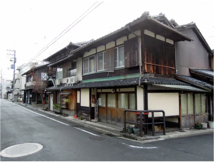
The houses of common people developed differently. Farmers in different regions of the country had houses that were adapted to local conditions. Some farmers' houses had space to keep their cattle and horses indoors, while the houses of city dwellers were often squeezed close together along the streets. As urban homeowners were taxed based on the width of the front side of the house, their houses were built to be long and narrow. This style can still be seen today in older cities like Kyoto. [14]

(27)

Figure 1.3: house in Kyoto

Traditional Japanese houses are built by erecting wooden columns on top of a flat foundation made of packed earth or stones.

In order to avoid moisture from the ground, the floor is elevated several tens of centimetres and is laid across horizontal wooden floor beams.

Areas like the kitchen and hallways have wooden flooring, but rooms in which people sit, such as the living room, are covered with mats called tatami that are made from woven rush grass. Japanese generally don't use chairs on top of tatami, so people either sit directly on the tatami or on flat cushions.

The frame of a Japanese house is made of wood, and the weight is supported by vertical columns, horizontal beams, and diagonal braces. Diagonal braces came to be used when the technology of foreign countries was brought to Japan.

(28)

One representative characteristic of houses in Japan is that they have a large roof and deep eaves to protect the house from the hot summer sun, and the frame of the house supports the weight of the roof.

Internal walls are really thin and the columns are not tapered at all, these are common characteristics for Japanese constructions. [15]

Figure 1.4: traditional Japanese structure (cultorweb.com)

In the old days, the walls of houses were made of woven bamboo plastered with earth on both sides. Nowadays, though, many different types of materials have been developed, and plywood is often used.

Also, in the past, many houses had columns that were exposed outside the walls. But in the Meiji era (1868-1912), houses came to be made using a method that encases the columns inside

(29)

roofs seen in different areas of Japan, they all have one thing in common: they are sloped instead of flat, allowing rainwater to flow off easily.

Japanese houses have developed over the years by combining traditional forms with modern technology to make them more resistant to fire and to improve their economic convenience. Recently, though, people are beginning to look anew at the traditional methods of building houses, which are easy on the environment and last a long time. [14]

(30)

2 Japanese seismic design code

The seismic design of Japanese buildings, (MLIT 2013, The Building Standard Law of Japan Enforcement Order) is featured by a two-phase design for earthquakes. (Hasegawa T., 2013; Aoyama H., 1981; Nakano K. et al, 1980; Ishiyama Y., 1980; Umemura H., 1979)

The first phase aims at the safety and reparability of buildings during medium earthquake motions. The second phase design for earthquakes is added to give safety against severe ground shaking.

Figure 2.1 shows the general flow of structural design stipulated by the current Enforcement Order of the Building Standard Law. All buildings are first divided into four groups, mainly based on their heights. They are shown in the boxes marked as (1)–(4).

For buildings taller than 60 m, in box (4), provisions of the Building Standard Law do not apply directly. These high-rise buildings are to be designed by the “special study”, usually incorporating time-history, non-linear response analysis.

For buildings not exceeding 60 m in height, the basic intent of the general flow is to make a two-phase design. This means that an additional design phase, hereafter called the second phase design for earthquakes, follows the working stress design, including the seismic design, hereafter called the first phase design for strong earthquakes which can occur several times during the life time of the building. The second phase design is intended mainly for severe or extraordinary earthquakes which could occur once in the lifetime of the building.

For all of these buildings, working stress design is carried out first, box (5), including the first phase seismic design.

Box (1) is for buildings of the most prevalent construction type in Japan. They include low-rise buildings of reinforced concrete with a generous amount of shear walls. For these buildings there is ample experience in Japan in seismic design and also evidence of seismic behaviour. The first phase design, basically unchanged from the rules of the former building code, should be successful in providing sufficient seismic resistance for these buildings to withstand severe earthquakes. Hence the second phase design need not be applied to these buildings.

(31)

Figure 2.1: traditional Japan

For buildings of boxes (2) and (3), the second phase design follows. The most important step in the second phase design is the evaluation of ultimate capacity for lateral load in box (9). The evaluation of story drift, box (6), is intended to eliminate soft structures which might experience excessively large lateral deflection under the seismic loading.

For buildings whose height is up to 31 m, box (2), there is a choice of flow into boxes (7) and (8), or into box (9). Box (7) requires a check for the rigidity factor and the eccentricity. The rigidity factor refers to the vertical distribution of lateral stiffness. The purpose of this check is

(32)

to eliminate buildings with one or more soft stories among the other stories, such as the soft first story. Checking for eccentricity is necessary to provide protection against excessive torsional deformation. These checks are followed by satisfying a set of additional minimum requirements specified by the MLIT, box (8), to ensure certain levels of strength and ductility

(33)

2.1 First phase design for earthquake

2.1.1 Load combinations and design method

The first phase design for earthquakes, as shown in box (5) of Figure 2.1, is a part of working stress design as prescribed by the Enforcement Order of the Building Standard Law, which considers under usual circumstances five kinds of loading.

These are: dead load, D; live load, L; snow load, S; wind forces, W; and seismic force, E. For permanent loading, the following load combinations are considered:

F=D+L

F=D+L+S (in designated snowy areas)

For short (temporary) loading, the following load combinations are considered: F=D+L+S

F=D+L+W

F=D+L+S+W (in designated snowy areas) F=D+L+E

F=D+L+S+E (in designated snowy areas)

The design is still based on the working stress design method.

The design for shear is based on an empirical equation derived from the ultimate shear strength. The design shear force is taken as the smaller of the shear force associated with the flexural yielding of the member (in case of columns yielding of the column at one end and the yielding of beams at the other end of the column may be assumed) or the shear force calculated using factored earthquake load.

(34)

2.1.2 Evaluation of seismic force

The chief revision in 1981 of the first phase design for earthquakes was in the method of evaluating lateral seismic force, Q. This is calculated as the seismic shear at an i-th level of a building with the following equation:

Qi =Ci

∑

Wi with i from 1 to n

C_i= ZR_tA_iC₀ Where:

Qi = seismic shear force at i-th story 

Wi=weight of i-th story (This includes dead load plus reduced live load and, if located in the designated snowy zone, reduced snow load.)

n = number of stories 

Ci = shear coefficient at i-th story  Z = seismic zone factor

Rt = vibration characteristics factor Ai = vertical distribution factor  C0 = standard shear coefficient

(35)

2.1.3 The seismic zone factor

The seismic zone factor Z is shown in Figure 2.1.3.1. The zoning was published in 1978. It is based on the most recent assessment of seismicity over Japan at that time. As seen in this figure, the value of Z=0.7 is the smallest, and is applicable only to Okinawa Islands.

The large cities such as Tokyo, Osaka and Kyoto are within the zone A where Z = l.0.

(36)

2.1.4 The vibration characteristics factor

The vibration characteristics factor Rt is a function of natural period, T and the type of subsoil. It is evaluated using the following equations:

R_t=_{1 when T ²Tc} R_t= 1.0 − 2.0(₍₎( − 1)2

when_{Tc <T²2Tc} Rt= 1.6()( when T>2Tc T

Where T is the fundamental natural period in seconds, and Tc is the critical period in seconds, determined according to the type of subsoil.

The fundamental natural period is calculated by the following expression:

T =(0.02+0.01a)h

where,

h = height of the building in meters 

a = ratio of the height of story, consisting of steel columns and girders, to the entire height h.

(37)

When the period of vibration is more accurately evaluated by a suitable method, or the vibration characteristics coefficient Rt is evaluated by a special study considering structural behaviour during earthquakes, such as soil–structure interaction, the value of Rt may be taken less than the value given by the previously equations, yet limited to be 3/4 of the value given by these equations.

(38)

2.1.5 Story shear force distribution factor along building height Ai

The vertical distribution factor Ai specifies the distribution of lateral seismic forces in the vertical direction, and is calculated by the following expression:

Ai=1+(,_-− 𝑎i)_,01(/( where, 

ai = non dimensional weight (or height) by the following expression:

ai= 2 3 454 6 2 3 457 6 where, 

Wi = weight of i-th story n = number of stories

As seen in Figure 2.1.5.1, the vertical distribution factor is close to a uniform value for shorter periods. Larger lateral force is assigned to the upper part of a building with long period. When the vertical distribution of seismic force is evaluated by a special study considering the dynamic characteristics such as spectral modal analysis, the equations in this subchapter need not be applied.

(39)

2.1.6 Standard shear coefficient

The standard shear coefficient C0 has been determined to not be less than 0.2 for the first phase seismic design. An exception is the case of wooden buildings in designated soft subsoil areas, when the value of C0 must not be less than 0.3.

Experimental earthquakes with Japan Meteorological Agency (JMA) of intensity 4 and 5 have shown that the majority of these buildings have behaved satisfactorily, and were almost without damage. The purpose of the first phase design is now to protect buildings in case of earthquakes which can occur several times during the life of the building. Such earthquake motions may be considered as having seismic intensity 5 on the JMA intensity scale, with the maximum acceleration of 80–100 cm/s2. Buildings are expected to respond to earthquakes of this level without loss of function. This design objective is assumed to be achieved by the first phase design.

The second phase design is intended to ensure safety against an earthquake which could occur once in the life time of the building. Such earthquake motion may be as strong as that of the 1923 Kanto earthquake in Tokyo, whose seismic intensity of upper 6 or even 7 in terms of JMA intensity scale with the maximum acceleration of 300–400 cm/s2. The traditional seismic design, as prescribed by the previous Enforcement Order before 1981, did not include direct evaluation of safety against such earthquake motions.

It was expected that buildings designed under seismic coefficient of C0 = 0.2 would safely survive severe earthquakes as a result of built-in over strength and ductility. Whether the structure possessed adequate levels of over strength and sufficient ductility was not expressly required to be confirmed.

Recent experiences in major earthquakes, such as the 1968 Tokachi Oki earthquake or the 1978 Miyagi-ken Oki earthquake, have shown in fact that the majority of Japanese buildings had adequate over strength and ductility to survive without any damage or with only minor damage. However, about 10 % of the affected buildings suffered notable damage and several buildings among these reached the stage of collapse.

(40)

2.1.7 Seismic force acting in the basement

The Building Standard Law also contains provisions for the seismic force to be considered for basements. Unlike the seismic shear force for the upper portion of buildings, the seismic force in the basement is calculated as the inertia force acting at the basement of the building directly, by multiplying the sum of the total dead and live loads for the basement, WB , by the following seismic coefficient:

k≥0.1(1- _9:8)Z where,

k = horizontal seismic coefficient 

H = depth from the ground level in m measured to the bottom of the basement, but it shall not be taken more than 20 m

Z = seismic zone factor

The story shear force QB at any basement level may then be calculated as follows: QB=Q’+kWB

where,

Q’=the portion of seismic story shear force in the adjacent upper story that is carried by columns and shear walls directly above the basement being considered

WB = weight of the basement story considered 

(41)

2.2 Buildings for which the second phase design is not required

Besides timber construction, they include the following, according to the specification of the MLIT:

1. Masonry buildings with not more than three stories, excluding the basement. 

2. Reinforced concrete block masonry buildings with not more than three stories, excluding the basement.

3. Steel buildings:

a) Not more than three stories, excluding the basement.  

b) Not more than 13 m in height, and not more than 9 m at eaves height.  

c) Horizontal distance between major vertical structural supports is not more than 6 m.  

d) Total floor area is not more than 500 m2.  

e) Design seismic shear force in the first phase design is calculated with the standard shear coefficient taken not less than 0.3.  

f) End connections and joints of braces carrying components of horizontal earthquake forces must not fracture when the bracing member yields.  

g) Not more than two stories, excluding the basement.  

h) Not more than 13 m in height, and not more than 9 m at eaves height.  

i) Horizontal distance between major vertical structural supports is not more than 12 m.  

j) Total floor area is not more than 500, or 3000 m2 in case of flat.  

k) Design seismic shear force in the first phase design is calculated with the standard shear coefficient taken not less than 0.3.  

l) End connections and joints of braces carrying components of horizontal earthquake forces must not fracture when the bracing member yields.  

(42)

4. Reinforced concrete buildings, steel reinforced concrete buildings, or buildings consisting in part of reinforced concrete and in part of steel reinforced concrete, not more than 20 m in height.

5. Buildings consisting of the mixture of two or more of the following constructions: timber, masonry, reinforced concrete block masonry and steel structures, or buildings consisting of any one or more of these above construction types and reinforced concrete or steel reinforced concrete construction, conforming to requirements below:

a) Not more than three stories, excluding the basement.  

b) Not more than 13 m in height, and not more than 9 m at eaves height.   c) Total floor area is not more than 500 m2.  

d) The story consisting of steel construction must conform to requirements (c),  (e) and (f) of item 3 above.  

e) The story consisting of reinforced concrete or steel reinforced concrete construction must conform to requirement (b) of item 4 above.  

6. Industrial (prefabricated) houses approved by the MLIT. 

7. Other construction approved by the MLIT as having equivalent or higher safety against earthquakes as the items listed above.

(43)

2.3 The Building Standard law of Japan Enforcement Order

-‐ Section 3 Wooden Structure

In the next pages is mentioned the Building Standard Law of Japan Enforcement Order, and it is explained in details the wooden structure design.

Article 46.

In buildings whose walls, columns and horizontal framing members constituting elements required for structural resistance are made of wood, frames having either walls or braces shall be arranged in well balanced on each floor in both the span and longitudinal directions so that the said buildings will be safe against horizontal force in any direction.

1. The provision of the preceding paragraph shall not apply to buildings or structural parts of buildings of wooden structure coming under any of the following items:

(1) Buildings or structural parts of buildings which conform to the criteria stipulated below: (a) The quality of glued laminated timber and other timber used as columns and horizontal framing members (excluding studs, small beams and other similar members; the same in this item) constituting elements required for structural resistance shall conform to criteria established by the Minister of Land, Infrastructure, Transport and Tourism concerning the strength and durability of the columns and horizontal framing members concerned. (b) The feet of columns constituting elements required for structural resistance shall be connected to sills connected to a monolithic continuous foundation constructed of reinforced concrete, or be connected to foundation constructed of reinforced concrete. (c) In addition to the above-mentioned items (a) and (b), structural safety has been conformed through structural calculation in compliance with the criteria established by the Minister of Land, Infrastructure, Transport and Tourism.

(2) Buildings with knee braces (limited to those fixed to columns which are reinforced with fish plate, etc.), stay posts and buttress walls which is satisfactory from the viewpoint of structural strength.

(44)

2. Corners of floor framing and tie beam framing shall be provided with angle braces and roof trusses with inter truss braces. Provided, that this shall not apply in cases where structural safety has been conformed through structural calculation specified by the Minister of Land, Infrastructure, Transport and Tourism.

3. In wooden buildings with two or more stories or with a total floor area exceeding 50 m2_, frames having either walls or braces to be arranged in both the span and longitudinal directions on each floor shall be installed in conformity with criteria specified by the Minister of Land, Infrastructure, Transport and Tourism so that the sum of the length obtained by multiplying the length of each frame in the same direction by one of the figures shown in the column of “Multiplier” of the following Table 1 according to the classification of frames as shown in the column of “Type of frame” of the said table, shall equal or exceed, in each direction, the value obtained by multiplying the floor area of the said floor (in a case where a storeroom is constructed on the said floor, the attic space or above the ceiling of the story above the said floor, or other similar space, the floor area obtained by adding a floor area specified by the Minister according to the floor area and the height of the said storeroom to the floor area of the said floor) by one of the figures shown in Table 2 (in areas designated by the Designated Administrative Agency under Article 88 paragraph 2, the figures will be 1.5 times those in Table 2) and also the value obtained by multiplying the plumb measure size (referred to as the “vertically projected area in the span or longitudinal direction”; hereinafter the same) of the said floor (including higher floors if any) minus the plumb measure size of the portion of the said floor up to a height of 1.35 m from the floor level, by one of the figures shown in Table 3.

(45)

Type of frame Multiplier (1) Frames with earth-plaster walls or frames with

walls with wooden lath or the like nailed to one side of columns and studs

0.5

(2) Frames with walls with wooden lath or the like nailed to both sides of columns and studs

1

Frames with a timber brace 1.5 cm or more in thickness and 9 cm or more in width or with a steel bar brace 9 mm or more in diameter

(3) Frames with a timber brace 3 cm or more in thickness and 9 cm or more in width

1.5

(4) Frames with a timber brace 4.5 cm or more in thickness and 9 cm or more in width

2

(5) Frames with a timber brace 9 cm or more square 3 (6) Frames with “X” braces shown in any of (2)

through (4)

Two times each value of (2) through (4)

(7) Frames with “X” braces shown in (5) 5

(8) Other frames approved by the Minister of Land, Infrastructure, Transport and Tourism or frames using a structural method specified by the Minister as having such strength as equal or superior to that of the frames shown in one of (1) through (7)

A value to be specified by the

Minister within the range between 0.5 and 5

(9) Frames with walls shown in item (1) or (2) and braces shown in one of (2) through (6)

The sum of the value of (1) or (2) and that of one of (2) through (6)

(46)

Buildings

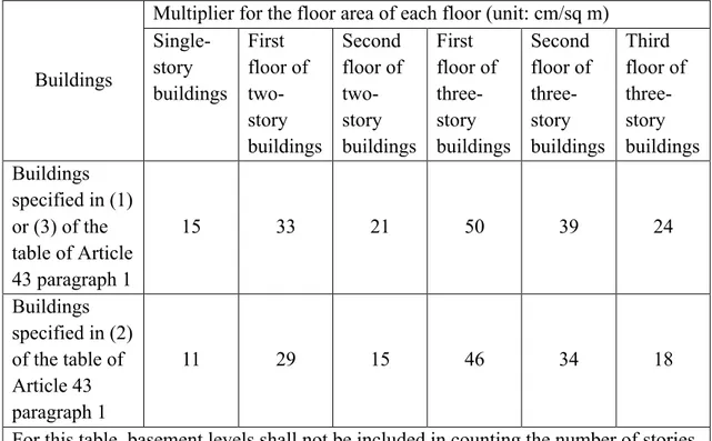
Multiplier for the floor area of each floor (unit: cm/sq m) Single-story buildings First floor of two-story buildings Second floor of two-story buildings First floor of three-story buildings Second floor of three-story buildings Third floor of three-story buildings Buildings specified in (1) or (3) of the table of Article 43 paragraph 1 15 33 21 50 39 24 Buildings specified in (2) of the table of Article 43 paragraph 1 11 29 15 46 34 18

For this table, basement levels shall not be included in counting the number of stories. Table 2.3.2: multiplier for the floor area

Areas multiplier for plumb measures size

(unit: cm/sq m) (1) Areas designated by the Designated

Administrative Agency by regulations as strong wind areas, based on past data on wind

A value to be determined by the Designated Administrative Agency by regulations based on the wind conditions in the region concerned within a range exceeding 50 and not more than 75 (2) Areas other than the above 50

Table 2.3.3: areas multiplier coefficients

Article 43.

The ratio of the smallest width of columns constituting elements required for structural resistance in the span direction and in the longitudinal direction in relation to the vertical

(47)

shall not apply in cases where a calculation that complies with criteria specified by the Minister of Land, Infrastructure, Transport and Tourism confirms that safe from the viewpoint of structural capacity. [12] Buildings Columns (1) (2) (3) Buildings of dozozukuri*2 construction or other similar buildings with especially heavy walls Buildings other than those in (1) whose roofs are covered with light materials such as metal sheets, stone plates, wooden boards or the like Buildings other than those in (1) and (2) Columns placed at intervals of 10 m or more in the span and longitudinal directions or columns in

buildings for use as schools, day nurseries, theaters, movie

theaters, entertainment halls, grand-stands, public halls, assembly halls, stores engaged in commodity sales (excluding those with an aggregate of floor areas of 10 sq m or less) or public bathhouses Columns in the uppermost story or columns of single-story buildings 1/22 1/30 1/25 Columns in other stories 1/20 1/25 1/22

Columns other than the above Columns in the Uppermost story or columns of single-story buildings 1/25 1/33 1/30

(48)

Columns in

3 Modelling and analysis of building tests

At the beginning the work started with the study of the building to be tested. This construction is the one used for the shaking table tests.

In the model every vertical planes are replaced by x-shaped braces. The ones in the red colour are called “wall of columns” and they have specific mechanical properties, the ones in the blue colour are called “braces” with their own mechanical characteristics.

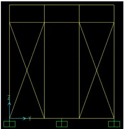
The other materials created with SAP2000 are called “beams” and “foundations”: the first one represents all the beams of the first floor while the second one represents the beams of the ground floor and also the columns of the specimen. They have different mechanical properties. The footprint of the structure is 3,43 m x 5,46 m and 2.8 m high with one story. The horizontal and vertical view of the tested building are shown in Figure 3.1 and Figure 3.2.

(50)

Figure 3.2: vertical view of the test’s building

As can be seen from the pictures this structure is quite simple and it is used in order to test and study in detail the mechanical characteristic of the Wall of Columns.

The exact properties are reached by the comparison between the displacement and the shear force of the real tests, and the model created with SAP2000.

Three different models were analysed: they have all the same plan and high dimensions but the first model has 8 Wall of Columns, the second model has 4 Wall of Columns and the third one has 2 Wall of Columns. These ways of retrofitting are placed in the plan that is shown below. The red walls represent the “Wall of Columns”, the blue walls represent the two-sided braces and the cyan walls represent the new smaller two-braces, placed in such a way to replace the old wall of columns.

The wooden frame remains the same during all the three tests, only the broken braces could be replaced by new ones.

(51)

Figure 3.3: horizontal view, 8 wall of columns

(52)

(53)

As previously mentioned, in SAP2000’s models the Wall of Columns are replaced by special braces with their own Young modulus and shear force. Their mechanical characteristics have been calibrated on the bases of the experimental results in order to be as close as possible, in terms of displacement and shear force, to the real experimental results.

Other braces are used in the model to replace the common walls of the building.

For these reasons in all the models there is no presence of structural plate elements, both vertical and horizontal.

For each model I studied and compared the results of different strengths of Kobe earthquake: starting from 10% of the ground motion to 20%, 40% and 80% of it.

(54)

3.1 SAP2000 model

This model was created with SAP2000. This general-purpose civil-engineering software is used worldwide for the analysis and design of structural systems, by a sophisticated finite-element analysis procedure.

First of all, the material property data should be determined, by creating an orthotropic material, in order to better simulate the behaviour of the wooden structure.

SAP2000 needs specific information, like the modulus of elasticity (three directions), the shear modulus, the Poisson’s ratio, the coefficients of thermal expansion and the density of the material, as shown in Figure 3.1.1.

(55)

For the duration of the analysis I controlled and changed the modulus of elasticity, the shear modulus and the damping coefficient in order to reach the same results of the shaking tables tests.

Parameters like Poisson’s ratio and the coefficient of thermal expansion remain the same in all the analyses and they are the ones proposed by SAP2000.

In Figure 3.1.2 all the frame properties can be seen which are found in the tested building. The dimensions are in millimetres.

Figure 3.1.2: frame properties

In Figure 3.1.3 the final 3D model can be seen.

The pictures below show that there are no roof or plate elements and the difference between the braces that represent the Wall of Columns can be seen as well as the real two-sided braces like in Figure 3.1.4 and Figure 3.1.5, where the perpendicular plane to X direction is shown.

(56)

(57)

Figure 3.1.4: vertical plan of the full-sized specimen with WoC, WoC side

(58)

The picture below shows the perpendicular plane to Y axis, the long side of the building. This is the chosen direction of the ground motion, so Kobe earthquake is applied in the Y axis, as the other researchers did in this tested building.

Figure 3.1.6: vertical plan of the full-sized specimen with WoC

In order to solve the so-called problem of the absence of the roof and to implement the plan’s stiffness of the first floor, a diaphragm was created. SAP2000 allows it to be created it by using the constraint function as shown in Figure 3.1.7.

(59)

Figure 3.1.7: diaphragm constraint

The ground joints used for the building are shown in the figure below.

Figure 3.1.8: joint restraint

(60)

previously, is taken 100% from the Kobe earthquake, and will be scaled each analysis (10%, 20%, 40% and 80%).

The final part of the ground motion was cut because the peaks are concentrated more or less in the first 30 seconds of the earthquake, so in the model 42 seconds are reported of Kobe earthquake in order to accelerate analysis process.

As reported in Figure 3.1.9, the value at equal intervals is 0,01 seconds, for a total time step number of 4221.

Figure 3.1.9: time history definition

(61)

Newmark presented a time-stepping method based on the following equations:

u°i+1 = u°i + (1-g)Dtüi + gDtü i+1 (1) ui+1 = ui + Dtui° + (0,5-b)Dt2üi + bDt2üi+1 (2)

Typical selection for g is ½, this is like taking a trapezoidal summation to get equation (1). Common selection for b includes ¼ which leads to the assumption of average acceleration during the time step and b equal to 1/6 which leads to the assumption of linear velocity over the time step. The final choice was for average acceleration with g=1/2 and b=1/4.

This is the most popular method for earthquake response analysis due to its superior accuracy; as the stiffness changes each time step, this kind of iteration is used to find the correct displacement within each time step.

In the end the vertical loads to the structure have been applied, in the same way of the real test. The total load is 6 tons and was applied as shown in the Figure 3.1.10: 1,5 tons distributed on the external beams, located on the perpendicular planes to X direction and 3 tons distributed on the central beam. This type of vertical load is considered a uniform load.

(62)

3.2 Modal analysis

After concluding the part regarding the construction of the model, the first thing that was done was to check the total weight of the structure (including 6 tons of vertical load), to analyse the modal shapes, check the periods and the frequencies and check the modal participating mass ratio.

All these values, extrapolated from SAP2000 model, need to be compared to the values of the experimental results, then the shear force and the displacement of chosen point of the structure can be analysed.

In Table 3.2.1 the total amount of the weight of the structure included the vertical loads can be seen (Global FZ). If it is not considered, the total weight of the tested building is close to 12 kN, like on SAP2000 model.

OutputCase CaseType GlobalFX GlobalFY GlobalFZ

Text Text N N N

DEAD, 6 TONS LinStatic 1,855E-‐12 1,023E-‐12 71355,35

Table 3.2.1: base reactions

In considering the other parameters, the period of the structure is shown in the table below: 0,265 seconds for the first mode, so the frequency is 3.77 s-1. In the real experiment the period is 0,25 seconds. It is verified that the behaviour of the real building is similar to the model created on SAP2000.

Moreover, 85% of activated mass in the X and Y directions is reached in the first three vibration modes and also for the rotation around Z axis, so the Italian seismic law is also verified.

(63)

Step Period[s] UX UY UZ RX RY RZ 1 0,268 0,92 0 0,000003822 6,688E-‐07 0,44 0,13 2 0,251 0 0,81 0 0,64 0 0,21 3 0,195 0 0,11 1,329E-‐19 0,08997 1,359E-‐20 0,59 4 0,057 0,000003582 6,931E-‐17 0,35 0,06202 0,15 5,144E-‐07 5 0,050 0,000006529 1,406E-‐15 0,000009112 0,000001594 0,000000381 9,377E-‐07 6 0,050 0,000504 5,607E-‐15 0,00006798 0,00001189 0,00003347 0,00007239 7 0,043 4,518E-‐15 0,0008951 6,705E-‐15 0,02057 2,283E-‐15 0,0004949 8 0,042 0,0000144 9,086E-‐15 0,21 0,03598 0,00001699 0,000002069 9 0,033 6,396E-‐15 0,0000298 7 7,918E-‐14 0,002182 1,335E-‐13 0,00004509 10 0,033 2,703E-‐15 0,0000514 1 5,562E-‐13 0,002045 3,13E-‐13 0,000000033 11 0,032 0,00001038 4,717E-‐17 0,19 0,03256 0,3 0,000001491 12 0,032 1,191E-‐15 0,0001821 9,356E-‐14 0,009332 8,948E-‐14 1,564E-‐07

Table 3.2.2: modal parameters

The first two periods are really close to each other so the stiffness is well distributed on the structure of the building. The first 3 modes activate the 85% of the participant mass, that satisfies the request of the Italian and European code.

The fourth mode is torsional, therefore it has very little effect on the structure.

The period is quite long taking into account that the specimen is 3 metres tall, so the building is quite deformable. It is reasonable that we don’t need to highly improve the stiffness of the entire structure with the wall of columns system.

(64)

3.3 Numerical versus experimental results

In this paragraph we will see the results of the SAP2000 model and the comparison between those values and the experimental results.

The first values that will be compared with the shaking table results will be the displacement – shear force plot.

At first the shape of the graphic will be compared: it was necessary to find a hysteretic behaviour of the wood and also the values of the peaks found in the model have to be close to the peaks values of the experiment (+- 20% of the experimental results).

Then the spectral ratio results will be compared. Even in this case the peaks studied in the SAP2000 model have to be close to the peaks of the experiment.

For 10% and 20% of Kobe earthquake strength, the final results are quite comparable, but for 40% and 80% cases it was more difficult to find good results because of a significant presence of noise in the experimental surveys and also for a high non-linear behaviour of the specimen. The non-linearity cannot be seen in a program such SAP2000, that is the reason why the purpose of this research is to control the displacement, not the exact shape of the wooden behaviour. First of all, there will be an illustration of the 8 Wall of Columns building starting from 10% of Kobe earthquake, then 20%, 40% and 80%. After that will be shown 4 and 2 Wall of Columns building results (always with the same percentage of Kobe earthquake strength).

In the figures below the orange lines are the results of SAP2000 model and the blue lines are the real experiment results.