Impact of PAMAM dendrimers on the photophysics of linked fluorophores: a spectroscopy and microscopy approach.

(1)

Universit`

a di Pisa

Facolt`

a di Scienze Matematiche Fisiche e Naturali

Corso di Laurea Magistrale in Fisica

Anno Accademico 2010/2011

Master Thesis

Impact of PAMAM dendrimers on the

photophysics of linked fluorophores: a

spectroscopy and microscopy approach

Candidate Advisor

Diana Di Paolo Dott.

(2)

Introduction

In the scientific world of today it is sometimes argued that the key to future progresses in Science lies in a more and more increasing specialization of individual areas of research, such as Mathematics, Physics, Biology and Chemistry. Although all these subjects may rightly undertake different roads in order to evolve our knowledge of Nature from differ-ent point of views, these paths should not be thought of as parallel. In fact, the most exciting and revolutionary discoveries may be waiting for us when they cross. Some of the most productive contributions to the advancing of science come from people who have developed a solid specialized background in either of the traditional disciplines, but have then pursued a horizontal research work, marked by interdisciplinar exchanges and cross-linking of knowledges.

Biophysics is a relatively new approach to the Life Sciences, founded on a strongly multi-disciplinary background of Biology, Chemistry and Physics. It focuses on the biochemical processes that characterize the carbon-based life, and aims to explain them as fully as possible trying to frame them in a theoretical model. In order to reach this goal, fluores-cence microscopy and spectroscopy, paticularly in time-resolved variants, are establishing as primary research tools. Some of the most recent and promising applications of Bio-physics are in the biomedical field. One of the scientists’ ultimate purpose would be realizing nano-devices capable of diagnosing and healing the single diseased cells, without involving the healthy ones. It is evident how nano-medicine would be much less inva-sive and much more accurate than its macroscopic counterpart. To achieve this goal, it is desirable to develop and create a multivalent dispositive composed by a scaffold that should be biocompatible and metabolizable by the body once its job is finished, and able to carry cell-penetrating targeting agents (peptides, antibodies, small ligands), sensing and/or imaging moieties (fluorophores or probes of other kind) and actuators (drugs or similar). In this view, many macromolecules have been proposed as building blocks for this nanotool, for example nanoparticles, nanotubes and dendrimers.

Dendrimers are highly branched synthetic polymeric molecules, with all bonds emanating radially from a central core with highly reproducible structure. They have revealed a con-siderable potential in several biological and biomedical applications; one of the interesting features of these macromolecules is that they have surface groups that can be successfully functionalized in a controlled way, e.g. with drugs, fluorophores, or other contrasting or sensing agents, in order to serve as biosensors in the cellular environment or as drug

(5)

carriers once they are internalized in living cells or organisms [1, 2].

This emerging scenario motivates the present thesis work. Indeed, while there exist many papers and works regarding (or even exploiting) fluorophore-functionalized den-drimers [3, 4], a careful analysis of the impact of denden-drimers on the photophysics of those fluorophores is still missing. In the work described in this thesis, several of the fluorescence techniques most widely used in Biophysics have been employed to study the physical-chemical properties of Polyamidoamine (PAMAM) dendrimers functional-ized with fluorescent dyes Carboxyfluorescein N-hydroxy succinimide ester (5(6)-FAM SE or NHS-carboxyfluorescein). In particular, the dendrimers used are of Generation 4 (G4) and have an ethylendiamine core. Beyond the classical spectroscopic techniques aimed at investigating absorption and fluorescence properties of the samples, three specific fluorescence microscopy techniques have been exploited: Fluorescence Lifetime Imaging Microscopy (FLIM), Fluorescence Correlation Spectroscopy (FCS) and Single Molecule Detection (SMD) [5].

The ultimate goal of this project is to study how the optical and mechanical properties of the samples may vary with respect to the dye alone also by tuning relevant parameters, such as the charge on the surface of the dendrimer (i.e. by acetylating the usually posi-tively charged amino end groups), the number of fluorophores on the surface, the pH, and other significant quantities that may affect the internalization, diffusion and the general behavior of dendrimers in cells.

In order to reach this goal, molar extinction coefficients of the charged samples and quan-tum yields of either charged and acetylated samples were determined; these values were compared with the known ones of the dye alone (also confirmed by measurements I per-formed firsthand). We found that the direct linkage to the dendrimer surface affects the optical properties of the dye by a similar extent for charged and neutral samples: in particular, we observed a strong decrease in its average quantum yield. Absorption and emission spectra at various pH were recorded; differences in the shape and peak wavelength of the spectra with respect to those of the non-conjugated fluorophore were interpreted as caused by interactions between the dye(s) and the dendrimer local envi-ronment. Finally, measurements performed by means of fluorescence microscopy (FLIM, FCS) and Single-Molecule techniques allowed us to better elucidate the results obtained with spectroscopy methods, reaching the following conclusions: there are interactions between NHS-carboxyfluorescein fluorophores bound directly to the surface of PAMAM dendrimers with the dendrimers themselves, which affect significantly the photophysical properties of the dyes; there are different configurations which cause different brightnesses for the dyes; these configurations seem to evolve dynamically in the single dendrimer-dye(s) systems, probably according to the ever-changing local conformation of these com-plexes.

(6)

CONTENTS 5

This thesis is organized as follows:

• Chapter 1 focuses on dendrimers, with particular attention to their chemical struc-ture, the unique features of the dendritic architecture and their biological applica-tions.

• Chapter 2 starts with a brief overview of the general theory that underlies the interactions between light and matter. In particular, I describe the processes of absorption and emission of radiation, the mechanism of fluorescence and its typical characteristics, such as lifetime, quantum yield and quenching. Then, the main spec-troscopic and fluorescence microscopy techniques exploited during the experimental part of this project are illustrated, with particular emphasis on the three mentioned above.

• In Chapter 3, after a brief outline of the chemical and optical properties of fluores-cein and its derivative dyes, the materials and methods are listed, and the obtained results reported, for each technique employed.

• Chapter 4 summarizes the main experimental results of this thesis work. In this chapter, a qualitative model of interpretation for the peculiar behavior of the system dendrimer-fluorophores is proposed and the evidences observed in the experiments are enclosed in a global descriptive frame.

(7)

(8)

Chapter 1

Dendrimers: promising tools for

biomedical purposes

1.1 The Dendritic Architecture

In organic chemistry, a dendritic macromolecule is a molecule whose structure is charac-terized by a high degree of branching that originating from a single focal point (core). The dendritic architecture is perhaps one of the most pervasive topologies observed on our planet. In biological systems, these dendritic patterns may be found at dimensional length scales measured in meters (trees), millimeters/centimeters (fungi) or microns (neu-rons). One of the reasons for such extensive mimicry of these dendritic topologies is that they manifest maximum interfaces for energy and nutrient extraction/distribution and for information storage/retrieval. At the nanoscale level, there are relatively few natural examples of this architecture. Examples are the glycogen’s and the proteoglycans’ hyper-branched structure for energy storage.

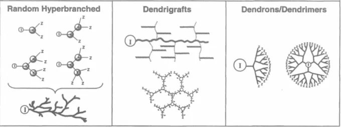
In chemistry, at least three major strategies are presently available for covalent synthesis of organic and related complexes beyond the atomic level, namely: traditional organic chemistry, traditional polymer chemistry and dendritic macromolecular chemistry. On the one hand, traditional organic chemistry leads to higher complexity by involving the formation of relatively few covalent bonds between small heterogeneous aggregates of atoms (reagents) to give well-defined small molecules. On the other hand, polymerization strategies involve the formation of relatively few covalent bonds between homogeneous monomers to produce large molecules with a broad range of structure control. All den-dritic polymers are open covalent assemblies of branch cells. There are three denden-dritic subclasses (Fig. 1.1): random hyperbranched polymers, dendrigraft polymers and den-drimers [6]. The order of this subset reflects the relative degree of structural control present in each of these dendritic architectures. In fact, hyperbranched polymers are polymers having imperfectly branched or irregular structures; dendrigrafts are the most recently discovered and currently the least well understood subset of dendritic polymers: they may be viewed as semi-controlled branched polymer architectures intermediate in terms of structure control between dendrimers and hyperbranched polymers. They most

(9)

often incorporate randomly distributed branching points, but are still characterized by narrow molecular weight distributions. Lastly, dendrimers have completely branched star-like topologies and display ordered structures with a high degree of reproducibility. Both dendrimer and hyperbranched polymer molecules are composed of repeating units ema-nating from a central core. In the following, I will restrict attention only on the third subclass, the one of dendrimers, which are the main subject of this thesis work.

Figure 1.1: Dendritic polymers: from left to right, random hyperbranched polymers, dendrigrafts and dendrimers.

1.2 Dendrimers: chemistry and structure.

Dendrimers are globular, nano-scaled macromolecules with a particular architecture con-stituted of three distinct domains, as illustrated in Fig. 1.3:

1. A central core which is either a single atom or an atomic group having at least two identical end groups;

2. An interior of shells consisting of repeating branch-cell units having at least one branch junction: their repetition is organized in a geometrical progression that re-sults in a series of radially concentric layers called generations (Fig. 1.4);

3. Many terminal functional groups, generally located in the exterior of the macro-molecule, which play a key role in the dendrimer’s properties.

The name dendrimer is derived from the Greek words dendri (branch tree-like) and meros (part of). In the past decade, over 2000 literature references have appeared on this unique class of structure controlled polymers. Poly(amidoamine) (PAMAM) den-drimers constitute the first commercialized dendrimer family and undoubtedly represent the most extensively charachterized and best understood series at this time. The core of PAMAM is a diamine (commonly ethylenediamine), which is reacted with methyl acry-late and another ethylenediamine to make the generation-0 (G-0) PAMAM (see Fig 1.2). Successive reactions create higher generations, which tend to have different properties.

(10)

1.2. DENDRIMERS: CHEMISTRY AND STRUCTURE. 9

Figure 1.2: PAMAM dendrimer production reaction: the ethylenediamine core reacts with methyl acrylate and another ethylenediamine yielding the G-0 PAMAM. In the figure, Me indi-cates a Methyl -CH3 group.

Intermediates during the dendrimer synthesis are denoted half-generations. The early generations (G= 1 − 3) possess a highly asymmetric, open, hemispherical shape, while the later generations (G≥ 4) possess a nearly spherical shape with dense-packed surface. Lower generations can be thought of as flexible molecules with no appreciable inner re-gions, while medium sized (G-3 or G-4) do have internal space that is essentially separated from the outer shell of the dendrimer. Very large (G-7 and greater) dendrimers can be considered more like solid particles with very dense surfaces due to the structure of their outer shell. The amine functional group on the surface of PAMAM dendrimers (Fig. 1.5) gives rise to many potential applications since they can be easily functionalized with any moiety presenting a reactive carboxyl group. In this thesis work we decided to employ this type of dendrimers; further description of the materials will be reported in Chapter 3, Section 3.2. The concept of repetitive growth with branching at molecular level was first reported in 1978 by V¨ogtle [7] (University of Bonn, Germany) and was followed closely by the parallel and independent development of the divergent, macromolecular synthesis (explained in Subsection 1.2.1) of true dendrimers in the Tomalia Group [8] (Dow Chem-ical Company). The first paper describing in detail the preparation of Poly(amidoamine) (PAMAM) dendrimers with molecular weights ranging from several hundred to over 1 million Daltons appeared in 1985 [9]. The appearance of this paper produced a rise of in-terest in dendritic polymeric architectures, although many of the major scientific journals tepidly welcomed the illustrated results. Indeed, at first they did not consider dendrimers such a promising discovery, neither believed them to exhibit new and perhaps unexpected physical-chemical properties different from other kinds of polymers. Fortunately, these initial suspicions were refuted in the subsequent years as dendrimers have become the subject of more and more studies and publications, and today many hundreds of research groups from diverse scientific disciplines have joined the field, leading to numerous ad-vances in the synthesis, analysis and applications of these polymers [6].

1.2.1 Synthesis: Divergent and Convergent Methods

The methods for assembling the dendrimers can be categorized as either divergent or convergent; both synthetic processes can control precisely the size and number of

(11)

Figure 1.3: Schematic three-dimensional projection of dendrimer-core shell architecture for G= 4.5 poly(amidoamine) PAMAM dendrimer with principal architectural components (I) core, (II) interior and (III) surface. The quantities Ncand Nbwill be defined in Section 1.3 of this Chapter.

Figure 1.4: Schematization of the concept of generation of a dendrimer.

branches on the dendrimer. The first dendrimers were made by divergent synthesis ap-proaches; in 1990 a convergent synthetic approach was introduced by Jean Fr´echet. Fig. 1.6 illustrates both the divergent and the convergent method: in the former, the den-drimer is assembled from a multifunctional core, which is extended outward by a series of reactions; each step of the reaction must be driven to full completion to prevent mis-takes in the dendrimer, which can cause architectural defects (for example, some branches could be shorter than others); in the second, dendrimers are built from small molecules that end up at the surface of the sphere, and the reactions proceed inward up to the final attachment to a core. This method makes it much easier to remove impurities and shorter branches along the way, so that the final dendrimer is more monodisperse. However den-drimers made this way are not as large as those made by divergent methods because are more subject to crowding due to steric effects. Ideally, a dendrimer can be synthesized to have different functionality in each of its three portions (core, interior and surface) to control properties such as solubility, thermal stability, and attachment of compounds for particular applications. PAMAM dendrimers are synthesized by the divergent approach.

(12)

1.3. UNIQUE FEATURES OF DENDRIMERS. 11

Figure 1.5: G-2 poly(amidoamine) (PAMAM) dendrimer and detail of the amine terminal group.

Figure 1.6: Schematic of divergent and convergent synthesis of dendrimers.

1.3 Unique Features of Dendrimers.

Dendrimers are unique nanoscale devices. Their three components (core, interior and terminal groups) determine their physical-chemical properties, as well as the overall size, shape and flexibility. It is important to note that dendrimer diameters increase linearly as a function of generation, while the number of surface functional groups increases expo-nentially. We define now two quantities of interest to describe the dendrimer structural properties: the core multiplicity Nc and the branch cell multiplicity Nb, the number of

(13)

These quantities contribute to determine the precise number of terminal groups Z and of covalent bonds formed as a function of generation G, according to

Z = NcNbG (1.1)

Nbonds= Nc

NbG− 1

Nb− 1

(1.2) The surface groups (Z) and number of bonds amplify mathematically according to a power function of the generation, producing structures with precise molecular weights, as shown in Table 1.1.

Table 1.1: Theoretical number of surface groups (Z), molecular formulas and weights calculated by means of Eqs. 1.1, 1.2 for a PAMAM dendrimer, cystamine core. The molecular weights approximately double as one progresses from one generation to the next.

1.3.1 Comparison with Traditional Polymers

Unique features offered by dendrimers that have no equivalency in the linear topologies include:

1. Nearly complete monodispersity (the property of an ensemble with constituents all with the same mass): although, in general, convergent methods yield the most nearly isomolecular dendrimers, mass spectroscopy has shown that PAMAM dendrimers produced by the divergent method are very monodisperse;

2. The display of unimolecular container/scaffolding properties; 3. Exponential amplification of terminal functional groups;

4. Persistent nanoscale dimensions as a function of molecular weight (generation). Apart from those reported above, which are exclusive characteristics of dendrimers, the dendritic architecture presents other properties which differ from those of linear polymers; let’s list the most peculiar of these: first, the solubility of the latter decreases with molec-ular weight, whereas for dendrimers it increases; second, in contrast to what normally observed for linear polymers, viscosities of dendrimers do not increase continuosly with

(14)

1.4. DENDRIMERS FOR BIOLOGICAL APPLICATIONS 13

molecular weight, but reach a maximum at a certain generation; lastly, dendrimers present isotropic electronic conductivity, whereas linear polymers usually show an anisotropic elec-tronic conductivity. To conclude, I shall say that the properties of dendrimers result in

Figure 1.7: Schematic comparison of a common linear polymer (like plexiglas or nylon) and a dendrimer.

large part dominated by the functional groups on the molecular surface; however, there are examples of dendrimers with internal functionality [10]. It is possible to make den-drimers water soluble, unlike most polymers, by functionalizing their outer shell with charged species or other hydrophilic groups. Other controllable properties of dendrimers include toxicity, crystallinity, and chirality [11].

1.4 Dendrimers for Biological Applications

The last decades have seen research at the interface between polymer chemistry and the biomedical sciences giving birth to the first nano-sized (5-100 nm) polymer-based phar-maceuticals. This family of constructs has been called ”polymer therapeutics”. Polymer therapeutics are complex technologies, often combining several components, e.g., poly-mers, drugs, peptides, proteins and others. [12] The advent of dendrimer chemistry has brought many potential advantages to this new approach to therapeutics. In fact, unlike traditional polymers, dendrimers can be obtained in precise molecular weights even at high generations, which can provide a reproducible pharmacokinetic behavior. Plus, it is possible to conjugate other chemical species to the dendrimer surface in order to serve as detecting agents (such as a dye molecule), targeting components, imaging agents, or phar-maceutically active compounds. Recently, progress has been made also in the application of biocompatible dendrimers to cancer treatment, including their use as delivery systems for potent anticancer drugs. The field of biomedical dendrimers is still in its infancy, but the interest in dendrimers as active therapeutic agents, as vectors for targeted delivery of drugs, peptides and oligonucleotides, and as permeability enhancers able to promote oral and transdermal drug delivery is increasing at a fast rate. Scientists have also studied dendrimers for use in sensor technologies. Studied systems include pH or ionic sensors using dendrimer-dye composites to detect fluorescence signal quenching. We exploit this sensor feature of dendrimer-dye(s) systems later in this thesis, in Chapter 3, Section ??. Research in this field is vast and ongoing due to the potential for multiple detection and

(15)

binding sites in dendritic structures.

1.4.1 Drug Delivery

The physical characteristics of dendrimers, including their monodispersity, water solubil-ity, encapsulation abilsolubil-ity, and large number of functionalizable peripheral groups, make these macromolecules appropriate candidates for evaluation as drug delivery vehicles. Dendrimers have very strong potential for this application because, as already mentioned, their structure can lead to multivalent systems. In other words, one dendrimer molecule has hundreds of possible sites for coupling to active species. There are presently three methods for using dendrimers in drug delivery, as shown by Fig. 1.8: the drug can be covalently attached to the periphery of the dendrimer, coordinated to the outer functional groups via ionic interactions, or the dendrimer itself can act as a unimolecular micelle by encapsulating a pharmaceutical through the formation of a dendrimer-drug supramolec-ular assembly [13]. Indeed, dendrimers with hydrophobic core and hydrophilic periphery have shown to exhibit micelle-like behavior and container properties in solution[14]. This analogy highlighted the utility of dendrimers as solubilizing agents: in fact, the majority of drugs available in pharmaceutical industry are hydrophobic. This drawback of drugs can be obviated by dendrimeric scaffolding, which can be used to encapsulate as well as to solubilize the drugs because of the capability of such scaffolds to participate in exten-sive hydrogen bonding with water [15, 16]. The encapsulation increases with dendrimer generation and this method may be useful to entrap drugs with a relatively high thera-peutic dose. Studies based on dendrimers also open up new avenues of research into the further development of drug-dendrimer complexes specific for a cancer and/or targeted organ system.

Figure 1.8: Diagram showing schematically approaches for design of therapeutics and drug delivery systems [12].

(16)

1.4. DENDRIMERS FOR BIOLOGICAL APPLICATIONS 15

1.4.2 Gene Delivery

Gene delivery is the process of introducing foreign DNA into host cells. It is one of the main steps of genetic therapies. There are many different methods for gene delivery developed for various types of cells (from bacterial to mammalian) and tissues. Generally, the methods can be divided into two categories, viral and non-viral. Virus mediated gene delivery utilizes the ability of a virus to inject its DNA inside a host cell. A gene that is intended for delivery is packaged into a viral particle. Non-viral methods include physical methods such as microinjection and electroporation. It can also include the use of polymeric gene carriers. The ability to deliver pieces of DNA to the required parts of a cell presents many challenges. Current research is being performed to find ways to use dendrimers to traffic genes into cells without damaging or deactivating the DNA. PAMAM dendrimers have revealed to be highly efficient non-viral vectors for gene delivery into numerous cell lines, in vitro and in vivo, both as functionalized and micelle-like carriers [17]: some of their generations can be internalized in cells without inducing biocompatibility issues or toxicity and this confers to PAMAM dendrimers a significant advantage over other gene delivery vectors for use in vivo.

1.4.3 Biocompatibility and Toxicity

Surveys regarding the toxicology of dendrimers for biological and cellular environments are currently under development. The cytotoxicity (quality of being toxic to cells) of unmodified PAMAM dendrimers was found to be appreciably higher for cationic com-pared with partially or totally uncharged dendrimers and for both types increased with increasing size (generation) and concentration [18]. It has been observed that surface modified dendrimers with carbohydrates should make it possible to avoid the cytotoxic effects of cationic and high-generation dendrimers and to reduce the toxicity in cells by re-duction/shielding of the positive charge on the dendrimer surface [2]. In future it will only ever be possible to designate a dendrimer as ”safe” when related to a specific application. The so far limited clinical experience using dendrimers makes it impossible to designate any particular intrinsically ”safe” dendrimer. Although there is widespread concern as to the safety of nano-sized particles, preclinical and clinical experience gained during the de-velopment of polymeric excipients, biomedical polymers and polymer therapeutics shows that judicious development of dendrimer chemistry for each specific application will ensure development of safe and important materials for biomedical and pharmaceutical use.

(17)

(18)

Chapter 2

Light-Matter Interactions

Photoluminescence is the property of any substance of emitting photons from electroni-cally excited states upon absorption of radiation of appropriate wavelength. In most cases, emitted light has a longer wavelength, and therefore lower energy, than the absorbed ra-diation. Photoluminescence includes the phenomena of fluorescence and phosphores-cence, depending on the nature of the excited state.

Let’s examine fluorescence first, the real protagonist of this thesis. Absorption occurs from the ground state of a molecule, which is usually a singlet state. In excited singlet states, the electron in the excited orbital remains ”paired” (by opposite spin) to the sec-ond electron in the ground-state orbital. Decay to the ground state occurs by emission of a photon with rates typically around 108_s−1_{, so that a typical fluorescence lifetime is}

near 10 ns (10 × 10−9s). The lifetime (τ ) of a fluorophore refers to the average time the molecule stays in its excited state.

Phosphorescence is emission of light from triplet excited states, in which the electron in the excited orbital has the same spin orientation as the ground-state electron. Transi-tions to the ground state are forbidden (at least in the electric dipole approximation) and the emission rates are slow (103 _{− 1 s}−1_{), so that phosphorescence lifetimes are typically}

milliseconds to seconds.

In short, fluorescence has immediate effect and stops immediately after the light source is turned off, while phosphorescence’s effect continues even after cessation of the irradiation. Besides, phosphorescence is usually not seen in fluid solutions at room temperature. This is because there are many deactivation processes that compete with emission, such as non-radiative decay and quenching. We will consider them in more detail later in this chapter.

2.1 Primary and Secondary photophysical processes

At the beginning of the studies about the interactions between light and matter, Stark and Einstein stated that each molecule is excited by only one photon. Exceptions are the so-called multiphoton processes, in which the molecule absorbs two or more photons at the same time. The latter occur exclusively when the energy difference between the involved

(19)

states of the molecule is equal to the sum of the energies of the two photons. Two-photon absorption is a second-order, nonlinear process and differs from linear absorption also because the probability of absorption depends on the square of the light intensity. Moreover, it is usually several orders of magnitude weaker than linear absorption.

Following excitation, a molecule may udergo chemical reactions, and in this case the process is called ”photochemical”, or it may not, and it is then called a ”photophysical” process. In general, we write: A + hν −→ A∗ where the star indicates a species which is in an electronic excited state. All the processes that directly involve the A∗ species are classified as ”primary” [19]. A list is reported below.

• Luminescence (radiation emission): A∗ _{−→ A + hν}0

Usually the emitted photon has a longer λ than the exciting one (ν0 < ν) because part of the energy is lost in other ways.

• Ionization: A∗ _{−→ A}+_{+ e}−

It generally requires high energies (8-10 eV in organic molecules) and the eventual energy in excess may convert to cinetic energy of the emitted electron.

• Non-radiative decay: A∗ _{−→ A}

No photon has been emitted returning to the electronic ground state, nor any chem-ical reaction has occured. Evidently, the molecule still possesses a certain amount of energy in the form of vibrations, which may be dispersed by collisions with the surrounding environment. This energy dissipation occurs with production of heat. • De-activation or Quenching: A∗ _{+ B −→ A + B}

Deactivation or non-radiative decay depend on the presence of another species B (See also Section 2.4.3).

• Energy Transfer: A∗_{+ B −→ A + B}∗

This can occur without exchange of a photon (see Fluorescence Resonance Energy Transfer in section 2.4.4 of this chapter).

• Photoisomerization: A∗ _{−→ B}

The A species turns into the B isomer, eventually in its ground state. The energy in excess can be dissipated through interactions with other molecules.

• Photodissociation: A∗ _{−→ B + C}

Part of the incident photon’s energy is used to break the bond between B and C fragments, and the remainder goes in cinetic and translational energy of B and C. • Bimolecular reaction: A∗_{+ B −→ C + D}

As the reagents typically contain energy in excess with respect to the reaction prod-ucts, the latter would probably disperse this excess by collisions.

Many of the products listed above possess enough energy left to undergo further physical-chemical processes, called ”secondary” since they do not directly involve the A species.

(20)

2.2. RADIATION ABSORPTION AND B EINSTEIN COEFFICIENTS 19

2.2 Radiation Absorption and B Einstein coefficients

Light is a propagating oscillating electromagnetic field. Molecules contain distributions of charges and spins that are altered when they are exposed to light. We are usually in-terested in the rate at which the molecule responds to this perturbation. In the following, I shall restrict attention only to the electric field of light, although more rigorous treat-ments include magnetic effects as well. A typical chromophore (a molecular moiety that interacts with light) is small (∼ 10˚A) compared to the wavelength of light (say 5000˚A); thus one can ignore the spatial variation of the electric field within the molecule. The oscillating electric field can then be written as

E0 = E0eiωt (2.1)

where E0 is the maximum amplitude and ω is equal to 2πν with ν frequency of the

electric field in Hz. Suppose our system is originally in state Ψa, an eigenstate of the

time-independent Hamiltonian ˆH with energy Ea; light perturbs the system causing transitions

between Ψa and other states at a certain rate. In general, in quantum physics, Fermi’s

golden rule is used to calculate the transition rate (probability of transition per unit time) from one eigenstate n with energy En of a quantum system to another eigenstate

m with energy Em, due to a perturbation W:

Pn→m∼

2π

~ | < Ψn|W |Ψm > |

2 _δ(E

m− En± ~ω) (2.2)

where δ is the Dirac Delta functional. In order to derive the result, let’s consider a hypothetical molecule with only two states, Ψaand Ψb. Because light is a time-dependent

interaction, the time-dependent Schr¨odinger’s equation must be solved. The Hamiltonian can be written as

ˆ

H0 = ˆH + ˆV(t) (2.3) where the effect of the light appears entirely in ˆV(t). The wavefunction of the system in the presence of light must be a linear a combination of the two states, with time-dependent coefficients:

Ψ(t) = Ca(t)Ψae−iEat/~+ Cb(t)Ψbe−iEbt/~ (2.4)

Inserting this expression into the time dependent Schr¨odinger equation with Hamiltonian 2.3, we obtain (after some algebra):

i~(Ψae−iEat/~dCa/dt + Ψbe−iEbt/~dCb/dt) = ˆV(t)[Ψae−iEat/~Ca(t) + Ψbe−iEbt/~Cb(t)] (2.5)

Multiplying by Ψ∗_aeiEat/~ _{or Ψ}∗

beiEbt/~ and integrating over spatial coordinates, we obtain

two equations to evaluate Ca(t) and Cb(t):

(21)

i~ dCb/dt =< Ψb| ˆV|Ψa> Cae−i(Ea−Eb)t/~+ < Ψb| ˆV|Ψb > Cb (2.7)

The integrals symbolized by the angle brackets are taken over spatial coordinates only. To proceed further, let’s insert an explicit form for the perturbing potential ˆV(t). As already said, a molecule is perturbed by light because its distribution of electric charge is altered by the presence of the oscillating electric field E; for electrically neutral molecules, this charge distribution is in good approximation represented by the electric dipole, which in quantum mechanics is described by the operator ˆµ = P

ieiri where the sum runs

over each electronic charge ei at position ri. I will consider only the electronic part of

the wavefunction, since the positions of nuclei are assumed to be fixed and thus can be ignored. Let’s calculate now the transition rate from the state a to the state b: Imposing |Cb(0)|2 = 0 and |Ca(0)|2 = 1, the Eq. 2.6 becomes:

i~ dCb/dt = Ca < Ψb|ˆµ|Ψa > ·E0e−i(Ea/~−Eb/~−ω)t (2.8)

where E0 has been removed from the integrals because it is constant over the dimensions

of the molecules.

Let’s now calculate the probability Pb that the system is in state b at time t. The result,

for small E0 and, again, imposing |Cb(0)|2 = 0 is:

Pb = |Cb(t)| 2 = |< Ψb|ˆµ|Ψa > ·E0| 2 ~2 t2sin2[(Eb/~ − Ea/~ − ω)t/2] 2[(Eb/~ − Ea/~ − ω)t/2]2 (2.9) For t → ∞, we have that

t2sin2[(Eb/~ − Ea/~ − ω)t/2]

2[(Eb/~ − Ea/~ − ω)t/2]2

−→ 2πt δ(Eb/~ − Ea/~ − ω) (2.10)

where δ(Eb/~ − Ea/~ − ω) is a Dirac Delta functional. Because ~ω is the energy of the

light, transitions from a to b will be induced only when ~ω = hν = Eb− Ea with Eb− Ea

energy separation between the two states. The rate at which these transitions occur is just the rate of change of |Cb(t)|

2

in response to illumination with radiation centered about frequency ν, and it is constant for large values of t, since the probability for the molecule being in state b increases linearly with time. We can write the transition rate dPb/dt as

a product of two terms

dPb/dt = BabU (ν) (2.11)

where Bab is the transition rate per unit energy density of the radiation and U (ν) is the

energy density incident on the sample at frequency ν. Recalling that U (ν) = |E0| 2

/4π and that the average of |< Ψb|ˆµ|Ψa > ·E0|2 over all possible orientations of the molecules

dipole moments is just (1/3)| < Ψb|ˆµ|Ψa > |2|E0|2, we can evaluate Bab:

Bab = (2/3)(π/~2)| < Ψb|ˆµ|Ψa > | 2

(2.12) Noting that, following the same procedure, it is possible to determine also Bba, the rate

(22)

2.3. SPONTANEOUS EMISSION AND A EINSTEIN COEFFICIENT 21

at which energy is removed from the light will be

−dU (ν)/dt = hν(NaBab− NbBba)U (ν) (2.13)

where Naand Nb are the number of molecules per cm3 in states a and b, respectively. The

quantities Bab and Bba are called Einstein coefficients for absorption and stimulated

emission, respectively; it is Bab = Bba [20].

2.2.1 The Extinction Coefficient

In a typical light-absorption measurement, a monochromatic beam of intensity I0 and

wavelength λ impinges on a sample (usually a solution of sample molecules with known concentration in mol l−1) for a path length of l cm; the not-absorbed light has intensity I < I0, and is collected by an appropriate detector.

Consider a beam of light propagating perpendicularly to a layer of sample molecules thin enough (dl) to suppose the light intensity within it constant; then the fraction of light that is absorbed is

−dI/I = Cε0dl (2.14) where ε0 is called the molar extinction coefficient: it is independent of concentration for non-interacting molecules but is function of the frequency (or the wavelength) of the absorption spectrum. Integrating the left member of Eq. 2.12 between I0 and I and the

right one between 0 and l, we obtain

ln(I0/I) = Cε0l (2.15)

Converting this expression to log10, we derive the well-known Lambert-Beer Law

A(λ) ≡ log10(I0/I) = cε(λ)l (2.16)

with ε = ε0/2.303 and A absorbance or optical density of the sample. ε is usually mea-sured in l mol−1cm−1 and usually spaces between 1 and more than 105 _{l mol}−1_cm−1_.

Looking at Eq. 2.16, we conclude that concentrations ∼ µM should be used for absorp-tion measurements in cuvettes with a 1 cm path length (lateral dimension) in order to have A∼0.1.

2.3 Spontaneous Emission and A Einstein coefficient

Consider again a molecule with only two energy levels Sb and Sa: As already said in the

previous section, Bab = Bba.

If originally there are namolecules in state Saand nb in Sb, then the net rates of conversion

from a to b and b to a are naBabU (ν) and nbBbaU (ν), respectively. At equilibrium, these

rates must be equal, which implies na = nb, independent of radiation density. This is

(23)

the ground state Sa. It was Einstein who first proposed that, in order to resolve this

discrepancy, one could postulate a rate of spontaneous emission of photons from Sb. The

rate of this process Aab is called the Einstein spontaneous emission coefficient and should

be independent of U (ν). When spontaneous emission is included and at equilibrium, we have

na/nb = [BbaU (ν) + Aba]/(BabU (ν)) = 1 + Aba/(BabU (ν)) (2.17)

Recalling that, according to the Boltzmann statistics, at thermal equilibrium it must be na/nb = e−(Ea−Eb)/KT = ehν/KT, with K = 1.38×10−23JK−1Boltmann constant, and that

at thermal equilibrium the energy density distribution of the electromagnetic radiation is that of a black body U (ν) = 8πhν3/[c3(ehν/KT − 1)], we obtain:

na/nb = (1 + Aba(ehν/KT − 1)c3)/(8πhν3Bab) (2.18)

and setting this value equal to e(hν/KT )

Aba = 8πhν3c−3Bab (2.19)

Note that the dependence of Aba by the cube of the frequency causes most of the emission

to be due to spontaneous decay at the highest photon energies.

In the absence of radiation or any other type of de-excitation, it will be dnb/dt = −Abanb,

with solution nb(t) = nb(0)e−Abat with nb(0) population of state b at zero time. Thus, it

is possible to define the radiative lifetime or natural lifetime of Sb as

τR= 1/Aba (2.20)

From Eqs. 2.19-2.20 derives that the stronger the absorption, the faster the emission of fluorescent radiation. In general, the lifetime of the excited state is defined by the average time the molecule spends in the excited state before returning to the ground state (tipically times of ns). Note that Eq. 2.17 is valid only if the electronic state couple involved in absorption and emission is the same. In fact, this is not always the case, and more complex expressions have been developed to account for this.

The radiative (fluorescence) rate constant (kF) is equal to 1/τR and so we have

kF = Aba (2.21)

(24)

2.4. EMISSION SPECTRA AND THEIR PROPERTIES 23

2.4 Emission spectra and their properties

Absorption is an event which occurs so fast - ∼ 10−15s - that there is no time for molecular motion or for significant displacement of nuclei during it (Franck Condon principle). As a result, absorption spectroscopy can only yield information on the average structure of the molecules that absorb light and absorption spectra are not sensitive to molecular dynamics but can only provide information on the average local environment surronding the chromophore. Only solvent molecules that are immediately adjacent to the absorbing species will affect its absorption spectrum. Light emission can reveal properties of bio-logical molecules quite different from the ones revealed by light absorption. The process takes place on a much slower time scale, allowing a much wider range of interactions and perturbations to influence the spectrum. A fluorescence emission spectrum is a plot of the fluorescence intensity versus the wavelength λ (nm) or the wavenumber k = 1/λ (cm−1) of emitted light. The following sections will examine in more details the characteristics of fluorescence and the main factors that affect the emission intensity.

2.4.1 Jablonski Diagrams

The transitions between electronic states are usually displayed by the Jablonski di-agrams, named after Professor Alexander Jablonski, who is regarded as the father of fluorescence spectroscopy. In this schemes, each molecular level is indicated by a hori-zontal line, and the electronic levels are actually split in several horihori-zontal parallel lines, to represent the partition in rotational and vibrational sublevels. In Figure 2.2, radia-tive transitions (absorption, fluorescence, phosphorescence) are drawn as coloured arrows, non-radiative ones as black arrows. Horizontal arrows indicate processes that conserve energy, like conversions, e.g. from electronical to vibrational excited states in Internal Conversion (IC) and InterSystem Crossing (ISC), whilst vertical and oblique ones indicate exchange of energy with the electromagnetic field (absorption, stimulated emis-sion, photoluminescence) or with other molecules (collisions, solvent interactions). The non-radiative processes of Internal Conversion and InterSystem Crossing are outlined in more detail in the following subsections.

(25)

Figure 2.1: General form of a Jablonski diagram: it does not include non-radiative interactions such as quenching, energy transfer, and solvent interactions.

Figure 2.2: Jablonski diagram with collisional quenching and fluorescence resonance energy transfer (FRET). The term P ki represents non-radiative decay channels aside from quenching

and FRET.

2.4.2 Internal Conversion and Kasha’s Rule

Following radiation absorption, a fluorophore is excited to some vibrationally excited state of a higher electronic level SN. The decay from a molecular state to a lower one

with the same spin molteplicity is called Internal Conversion (IC). It is due to loss of energy by collisions with solvent or by dissipation through internal vibrational modes and thus increases as the temperature is raised. This process has typical times of 10−12 s or less, and thus occurs prior to emission, since fluorescence lifetimes, as already said, are around 10−9− 10−8 _{s. Hence, fluorescence emission generally results from a thermally}

equilibrated excited state, that is, the lowest energy vibrational state of S1. This causes the Kasha’s Rule, which states that the fluorescence spectrum is indipendent from the excitation wavelength; similarly, the quantum yields of most of the primary processes are also independent from the excitation wavelength. After excitation, the fluorophore returns to the electronic ground state, but usually on a vibrational level of higher energy, which then thermically relaxes to the fundamental one in about 10−12s. A consequence of the

(26)

processes explained above is that the energy of the emitted photon is usually lower than for the absorbed one. Another interesting consequence of emission to higher vibrational ground states is that the emission spectrum is typically a mirror image of the absorption spectrum of the S0 → S1 transition. This similarity occurs because electronic excitation

does not greatly alter the nuclear geometry. Hence the spacing of the vibrational energy levels of the excited states is similar to that of the ground state. As a result, the vibrational structures seen in the absorption and the emission spectra are similar.

2.4.3 InterSystem Crossing and Phosphorescence

Molecules in the S1 state can also undergo a spin conversion to the first triplet state T1. Emission from T1 can occur either by phosphorescence, or by internal conversion, and, since the triplet state generally is lower in energy than the excited singlet, phosphorescence is usually shifted to longer wavelengths relative to fluorescence. Conversion of S1 to T1 is an example of Intersystem Crossing (ISC). Transition from T1 to the singlet ground state is forbidden in electric dipole approximation, and as a result the rate constants for triplet emission are several orders of magnitude smaller than those for fluorescence, and therefore the triplet state will display an extremely long radiative lifetime (seconds or longer instead of nanoseconds typical of excited singlets). This means that collisions with other molecules or internal conversion can effectively compete with phosphorescence. This is why it is rarely observed in solution, but rather in solid and de-oxygenated samples, conditions very far from the biological ones in which we are interested.

2.4.4 Quenching of Fluorescence

Fluorescence quenching refers to any process that decreases the fluorescence intensity of a sample. The extent of quenching can be affected by the environment surrounding the fluorophore; in fact, a variety of molecular interactions can result in quenching. These include excited-state reactions, molecular rearrangements, energy transfer, ground-state complex formation, and collisional quenching. The latter occurs when the excited-state fluorophore is deactivated upon contact with some other molecule in solution, which is called the quencher. The molecules are not chemically altered in the process. When many fluorophore molecules are really close, they may also undergo self-quenching, which in general is quenching of an excited atom or molecular entity by interaction with another atom or molecular entity of the same species. This concept will be resumed in Chapter 4. For collisional quenching the decrease in intensity is described by the Stern-Volmer equation:

F0

F = 1 + K[Q] = 1 + kQτ0[Q] (2.22) where F0 and F are the fluorescence intensities in the absence and presence of quencher,

respectively, K is the Stern-Volmer quenching constant, which indicates the sensitivity of the fluorophore to a quencher, kQ is the bimolecular quenching constant, τ0 is the

(27)

lifetime of the fluorophore in the absence of quencher, and [Q] is the quencher concentra-tion. A fluorophore inserted in a macromolecule is usually inaccessible to water soluble quenchers, so that the value of K is low. Larger values of K are found if the fluorophore is free in solution or on the surface of a biomolecule, as in this thesis work. A wide va-riety of molecules can act as collisional quenchers. Examples include oxygen, halogens, amines. The mechanism of quenching varies with the fluorophore-quencher pair, but, in any case, it requires molecular contact between fluorophore and quencher. This contact can cause a (meta)stable nonfluorescent complex formation which produces the so-called static quenching, or can be due to diffusion or molecular collisions for the molecule in the excited state, fluorophore-solvent interactions and/or rotational diffusion (which will be described in Section 2.5), which result in dynamic quenching instead.

The measurement of fluorescence lifetimes is the most definitive method to distinguish static and dynamic quenching. Static quenching removes a fraction of the fluorophores from observation. The complexed fluorophores are nonfluorescent, and the only observed fluorescence is from the uncomplexed fluorophores. The uncomplexed fraction is unper-turbed, and hence the lifetime is τ0. Therefore, defining τ as the time constant in presence

of quencher, we have that for static quenching τ0/τ = 1. In contrast, for dynamic

quench-ing we have F0/F = τ0/τ .

One additional method to distinguish static and dynamic quenching can be based on careful examination of the absorption spectra of the fluorophore. Collisional quenching only affects the excited states of the fluorophores, and thus no changes in the absorption spectra are expected. In contrast, ground-state complex formation will frequently result in perturbation of the absorption spectrum of the fluorophore. In fact, a more complete treatment should include the possibility of different extinction coefficients for the free and complexed forms of the fluorophore. However, in many instances the fluorophore may be quenched both by collisions and by complex formation with the same quencher.

2.4.5 Resonance Energy Transfer (RET)

Another important process that occurs in the excited state and causes loss of energy is resonance energy transfer (RET), sometimes also called Fluorescence Resonance Energy Transfer (FRET). This process can occur if the emission spectrum of a flu-orophore, called the donor, overlaps with the absorption spectrum of another molecule, called the acceptor, in its close proximity and with proper orientation of the dipoles. The acceptor does not need to be fluorescent. RET does not involve emission of light by the donor, is not the result of emission from the donor being absorbed by the acceptor; the donor and acceptor are coupled by a dipole-dipole interaction. For these reasons the term RET is preferred over the term fluorescence resonance energy transfer (FRET), which is also in common use. The extent of energy transfer is determined by the distance between the donor and acceptor, and the extent of spectral overlap. The latter is described in terms of the F¨orster distance R0, according to the following expression which we report

(28)

Figure 2.3: FRET Jablonski diagram showing energy transfer from the donor D to the acceptor A. Eventual InterSystem Crossing for the acceptor is also reported.

Figure 2.4: Example of two possible situations considering a FRET couple: if there is a spectral overlap between donor emission spectrum and acceptor absorption spectrum (left part of the figure) we have high fluorescence resonance energy transfer (RET) and donor quenching; if, instead, the two spectra do not overlap much (right part of the figure), there is low FRET and the donor’s brightness remains unaltered.

here for completeness without derivation R06 ∝ κ2_Q D nN Z 0 ∞ FD(λ)εA(λ)λ4dλ (2.23)

where QD is the quantum yield of the donor, n is the refractive index of the medium,

N is the Avogadro’s number and FD(λ) is the fluorescence intensity of the donor with

the total intensity (area under the curve) normalized to unity. εA(λ) is the extinction

coefficient of the acceptor at λ, which is typically in units of l mol−1cm−1. The term κ2 _{is a factor describing the relative orientation in space of the transition dipoles of the}

donor and acceptor, and is usually assumed to be equal to its average value 2/3, which is appropriate for dynamic random averaging of the donor and acceptor. This expression allows the F¨orster distance to be calculated from the spectral properties of the donor and

(29)

the acceptor and the donor quantum yield. The integral term in Eq. 2.23 expresses the degree of spectral overlap between the donor emission and the acceptor absorption. The rate of energy transfer kT(r) is given by ([5])

kT(r) = 1 τD (R0 r ) 6 _(2.24)

where r is the distance between the donor (D) and acceptor (A) and τD is the lifetime of

the donor in the absence of energy transfer. The efficiency of energy transfer for a single donor-acceptor pair at a fixed distance is

E = R0

6

R06+ r6

(2.25) Hence the extent of transfer depends on distance r. Fortunately, the F¨orster distances are comparable in size to biological macromolecules: 30 to 60 ˚A. For this reason, energy trans-fer provides an opportunity to measure the distances between sites on macromolecules. According to Eq. 2.25, the distance between a donor and acceptor can be calculated from the transfer efficiency.

2.4.6 Effects of Chemical Environment on Emission Spectra

Emission spectra are dependent upon the chemical structure of the fluorophore and the solvent in which it is dissolved (solvatochromism). This is caused by the different interactions between the fluorophore and the solvent itself, which change the energy of the ground and of the excited states of the molecules. In particular, in case of a polar solvent, its molecules orient themselves in order to reduce the ground state energy of the system. Since the charge distribution in the excited state is usually different than in the ground state, this orientation won’t be the one with minimal energy for the excited state. However, rotational motions of small molecules in fluid solution are rapid, typically occurring on a timescale of 40 ps or less. The relatively long timescale of fluorescence allows ample time for the solvent molecules to reorient around the excited-state dipole, which lowers its energy and shifts the emission to longer wavelengths. This process is called solvent relaxation and occurs within 10−10s in fluid solution. These increased differences between absorption and emission can also produce more substantial Stokes shifts.

2.5 Lifetimes and Quantum Yields

All of the nonradiative processes just described (internal conversion, intersystem crossing and quenching of various types) compete with fluorescence in depopulating the excited singlet state. This is the reason why the latter decays faster than expected by its radiative lifetime. If Sb(t) is the population of the excited singlet state b, kF the intrinsic

(30)

2.5. LIFETIMES AND QUANTUM YIELDS 29

processes, then we can write

−d(Sb)/dt = [kF + kIC + kISC + kQ]Sb (2.26)

with solution

Sb(t) = Sb(0)e−t/τF (2.27)

where Sb(0) is the concentration at time zero and τF is the observed fluorescence decay

time:

τF = [kF + kIC + kISC+ kQ]−1 (2.28)

Defining the fluorescence Quantum Yield φF as the number of emitted photons divided

by the number of absorbed photons, this is equal to the ratio between the rate of radiative emission and of excited state depopulation, therefore:

φF =

kF

kF + kIC + kISC + kQ

(2.29) Combining this expression with the definitions of τF and τR, we find

φF = τF/τR (2.30)

If τR is known, from a measurement of the fluorescence decay rate τF it is possible to

determine the quantum yield φF. More details on the techniques used to measure

fluo-rescence decays, and on more complicated types of measured decay curves, will be given in Subsection 2.6.4, together with the description of the set-up for fluorescence lifetime imaging (FLIM), used during this thesis work to measure fluorescence decay curves.

2.5.1 Brightness

The extinction coefficient tells us how much of the incident light will be absorbed by a given dye, and reflects the wavelength-dependent absorption characteristics indicated by the excitation spectrum of the fluorophore. Emission is increased with higher incident light absorption, meaning that fluorochromes with greater extinction coefficients tend to emit more intensely, and require less energy to adequately excite them. The quantum yield, which is a measure of fluorescence emitted per light energy absorbed, determines how much of this absorbed light energy will be converted to fluorescence. The product of these factors is defined as the brightness B of a molecule:

B = φF × ε (2.31)

Suppose that we have a sample which emits a certain fluorescence intensity and we mea-sure an average number of emitted photons Ncounts for a given configuration of light

(31)

recorded and the sample’s concentration c according to:

B = αNcounts/c (2.32)

with α multiplicative factor that accounts for instrumental geometry and efficiency. I will make use of Eqs. 2.31 and 2.32 further in this thesis, in Chapter 3, Section 3.7.4.

2.6 Fluorescence Microscopy

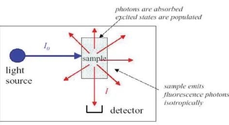
There has been a rapid growth in the use of microscopy due to advances in several tech-nologies, including probe chemistry (new types of molecular probes have been developed), confocal setups, detectors and computers. Most of the progresses reached during the last years in the field of microscopy stemmed from the purpose of increasing the contrast between the signal and the background in a measurement. In order to reach this goal, fluorescence microscopy is undoubtedly the most powerful technique, and this is one of the reasons why it has become a so widely used tool in the biological sciences. In a typical ap-plication of fluorescence microscopy, the chosen target is marked with a fluorescent probe (i.e. a fluorescent proteins or an organic dye); then, the marked target is internalized in the sample, for example cells, and the fluorescence emission is excited by means of a properly filtered source, observed with an optical microscope and collected by a detector (e.g. a CCD for wide-field microscopy), as illustrated in Fig. 2.5. The resolution of this

Figure 2.5: Typical experimental setup for an epifluorescence microscopy measurement. In epifluorescence, the sample is observed on the same side of illumination, therefore a dichroic is needed; this is a beam splitter that reflects excitation light and transmits emitted light.

type of microscopy is the same as that of common optical microscopy, but there is a gain with respect to the latter thanks to two factors:

(32)

2.6. FLUORESCENCE MICROSCOPY 31

1. the targeted markers localize only in specific cellular compartments, which are dis-tinguishable from the others because they are colored (enhanced contrast);

2. it is possible to mark different targets with different colors and then overlap the images in order to infer information from their colocalization (multichannel mi-croscopy).

Some applications of fluorescence microscopy suffer from the lack of knowledge of local probe concentrations within the sample. This led to the development of fluorescence microscopy techniques whose effectiveness is independent of concentration, such as Fluo-rescence Lifetime Imaging Microscopy (see Subsection 2.6.4 later in this chapter).

2.6.1 Confocal Microscopy

The resolution of a microscope determines the smallest feature that can be resolved, or the smallest distance that can be determined between two features. It depends on the used optics and microscopy configuration, but also on the signal-to-noise ratio (SNR), which is defined as

SN R = |mean signal − background|

signal standard deviation (2.33) where the background and the signal standard deviation values are increased by the effects of all kinds of noise, e.g. shot, thermal, photon scattering etc. A low SNR makes difficult to discriminate two spots very close to each other. The confocal variant of fluorescence microscopy was introduced to enhance three-dimensional optical resolution; in confocal microscopy, this is achieved by suppressing any signal coming from out-of-focus planes using a pinhole in front of the detector as schematically shown in Fig. 2.6. In a typical confocal setup, a collimated laser beam is reflected by a dichroic mirror and focused by a microscope objective to a small spot in the specimen; the emitted fluorescence is collected by the same microscope objective, transmitted by the dichroic, focused on the mentioned pinhole, eventually filtered and measured by a detector, which can be a photomultiplier tube (PMT), a photodiode or other light sensitive detectors. The effect of blocking out-of-focus fluorescence is called also ”optical sectioning” because it allows the imaging of separate slices within the sample. Only a single point is imaged at a time, so that to obtain a whole bidimensional section some kind of scanning is required. There are two ways for this: specimen scanning and laser scanning. In the former, the excitation beam is kept stationary while the object is moved, in the latter the sample remains steady and the excitation spot is moved. Laser scanning is usually the most employed method in confocal fluorescence microscopy. The utility of recording many optical sections of the sample is that these can be stacked by the computer to form tomographic images. A comparison between the result of widefield and confocal microscopy is shown in Fig. 2.7.

(33)

Figure 2.6: Schematic setup of a confocal microscope.

Figure 2.7: Comparison between a snapshot imaged with wide-field microscopy (left panel) and with fluorescence microscopy (right panel): in the latter, the noticeable high contrast enhance-ment is given by the absence of out-of-focus light.

2.6.2 The Point Spread Function (PSF)

The function of the objective and of the other lens in a microscope is to transform the diverging spherical wavefront radiated by the object to a converging spherical wavefront forming the image. Whereas the former extend over the full 4π radians of a sphere, the second is limited by the size of the lens, given by its aperture. The 3D distribution of light in the image of a point like source is called the Point Spread Function (PSF) of the optical system. For an ideal, aberration-free lens, the size of the PSF is determined only by the wavelength of the light and the numerical aperture of the lens (N A = n sin α, with n refractive index of the medium and α semi-aperture angle of focusing); in this case, the imaging is said to be diffraction-limited. The PSF can be calculated from diffraction theory; the Full Width Half Maximum of the PSF is said to determine the resolution limit, according to the Rayleigh criterion: two objects are spatially resolvable only if they

(34)

are more distant than it. This criterion is also expressed by Eq. 2.34: RES = 1.22λ

2 · N.A. (2.34) However, in principle it is possible to resolve two points that are closer than the FWHM by deconvolving the output signal with the PSF itself. Since it is nontrivial to calculate the PSF, it is widespread practice to evaluate it by fitting experimental data sets.

Figure 2.8: Schematic example of Point Spread Function.

2.6.3 Fluorescent Markers

Fluorophores are divided into two general classes, intrinsic and extrinsic. Intrinsic flu-orophores are those that occur naturally. Extrinsic fluflu-orophores are those added to a sample that does not display the desired spectral properties. A class of fluorophores con-sists of the fluorescent indicators, whose spectral properties are sensitive to a particular substance of interest. Whereas many organic substances present intrinsic fluorescence (autofluorescence), the typical microscopy approach is to employ extrinsic fluorophores. In the following, is reported a short list of the most common fluorescent markers used in flurorescence microscopy.

• Quantum Dots (2-10 nm in diameter, 102_{− 10}5 _{atoms): spherical structures made}

of nanocrystalline layers of semiconductor material (ZnSe, CdS, ecc) whose optical properties are linked to the formation of electron-hole pairs (excitons); their emis-sion wavelength are closely related to their linear dimenemis-sions. The new generations of quantum dots have far-reaching potential for the study of intracellular processes at the single-molecule level, high-resolution cellular imaging, long-term in vivo ob-servation of cell trafficking, tumor targeting, and diagnostics. The downside of using these objects as fluorescence probes in cellular environment is that, being artificial and made of inorganic elements, they are less biocompatible than other types of

(35)

markers listed below.

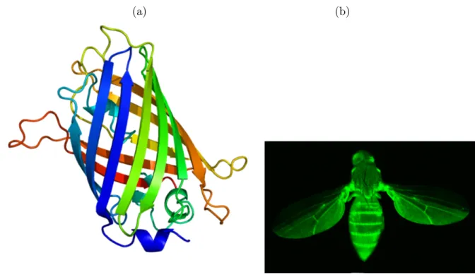
• Fluorescent Proteins (FPs, ∼26 kDa): intrinsically fluorescent, their name tradi-tionally refers to the Green Fluorescent Protein (GFP) first isolated from the jellyfish Aequorea victoria, which has a major excitation peak at a wavelength of 395 nm and a minor one at 475 nm. Its emission peak is at 509 nm and it has a fluorescence quantum yield of 0.79. As fluorescence probes, they have advantages and also dis-advantages: on the one hand, they can be genetically ”fused” to any other protein to be marked, and, once this is done, it is possible to create cell-lines or transgenic organisms that directly express the GFP labelled protein instead of the normal one, without significantly altering their physiology (Fig. 2.9). Thus, GFPs are very use-ful for in-vivo observations and, moreover, they are completely biocompatible and bond tightly to the targets. On the other hand, their fluorescence is less photostable and less etended than Quantum Dots one; plus, GFPs fluorescence shows a quite fast photo-bleaching (exponential decay of intensity upon protracted illumination).

(a) (b)

Figure 2.9: Green Fluorescent Protein barrel structure (a) and a bee genetically modified to express the GFP (b).

• Small organic molecules with delocalized electronic system: they often have ring structures (aromatic) or single-double bonds sequences, with π bonds which easily distribute outer orbital electrons over a wide area; this kind of molecules are ideal for fluorescence microscopy because the energy differences between the ground and excited states is small enough to allow relatively low-energy photons in the visible part of the electromagnetic spectrum to induce transitions from the first to the other. In general, the more interacting π bonds in the molecule, the smaller the energy gap

(36)

and higher the fluorescence quantum yield. An example is the Fluorescein and its derivatives, which are the fluorophores of interest in this thesis work. These molecules are chemically linked to the labelled objects and then are internalized in cells or employed in specific techniques that do not require internalization. I will discuss this type of fluorescent markers more in detail in Chapter 3, Section 3.1.

(37)

2.6.4 Fluorescence Lifetime Imaging Microscopy

As already anticipated in 2.5, time-resolved spectroscopy is a method of studying biophysical dynamic events investigating transient phenomena in the interaction of light with matter down to subnanosecond times. Time-resolved measurements contain more information than is available from the steady-state data. For instance, consider a sample containing two species, each with a distinct lifetime, but with spectral overlap of absorp-tion and emission; in this case, it is not possible to resolve the emission of the two from steady state data. However, the time-resolved data may reveal two decay times, which can be used to resolve the relative intensities and localization of the two species. Moreover, lifetime measurements allow to distinguish static and dynamic quenching, as anticipated in Subsection 2.4.4. Time-resolved measurements are widely used in fluorescence spec-troscopy, particularly for studies of biological macromolecules and increasingly for cellular imaging.

The Fluorescence-lifetime imaging microscopy (FLIM) technique was developed in the late 1980s and early 1990s (Bugiel et al. 1989, K¨onig 1989), before establishing as a fundamental in the late 1990s. It produces an image based on the difference between fluorescence exponential decays in various regions of the sample. It is a particularly useful technique because it provides measurements that are independent of probe concentration. In fact, the lifetime of a fluorophore is mostly independent of its concentration. Anyway, the fluorescence lifetime depends on environmental factors, such as ionic strength, oxygen concentration, hydrophobicity and interactions between the dyes and other molecules, especially if they result in FRET. In fact, FLIM can be used to measure FRET because the resonant passage of energy from the donor to the acceptor obviously decreases the donor’s lifetime. Since it is nontrivial to measure a single lifetime, the concept of lifetime imaging seemed impractical with the technology available in the 1980s and early 1990s. Even if such measurements could be performed, the data acquisition times would be ex-cessively long, precluding studies of living cells. At present, thanks to significant advances in technology, FLIM is establishing in the biosciences as a leading technique.

Measurement Methods for Decay Curves

The two classes of methods for measuring time-resolved fluorescence are time-domain and frequency-domain ones. In the first, the sample is excited with a short pulse of light, preferably much shorter than the decay time τ of the sample. A fluorophore which is excited by a photon will drop to the ground state with a certain probability based on the decay rates through a number of different (radiative and/or nonradiative) decay pathways, as already discussed in the previous sections. To observe fluorescence, one of these pathways must be by spontaneous emission of a photon. In the ensemble description, the fluorescence F(t) emitted will decay with time according to