Tesi di Dottorato in Economia Internazionale
-XIX Ciclo
Stefano Gerosa
Coordinatore Dottorato: Prof. Giancarlo Marini
Supervisore tesi: Prof. Pasquale Scaramozzino
Introduction v
Part 1. Knowledge Spillovers and the World Income Distribution 1
1. Introduction 2
2. The Model 5
3. The Equilibrium World Income Distribution 12
4. Conclusion 22
5. References 23
Appendix A. Existence and Uniqueness of the Equilibrium 25
Part 2. Knowledge Spillovers and Productivity Differences 31
1. Introduction 32
2. The World Income Distribution and Productivity Differences 34 3. The Structure of Knowledge Spillovers and Productivity Differences 37
4. Estimations and Results 42
5. Conclusion 45
6. References 46
Appendix A. Relative Factor Intensity, Relative Income and Relative
Productivity 49
Part 3. Capital-Skill Complementarity and Cross-Country Skill
Premia 59
1. Introduction 60
2. Capital-Skill Complementarity and the Skill Premium 61
3. The Skill Premium in the Steady State 64
4. Data, Estimation and Results 66
5. Conclusion 72
6. References 72
Appendix A. Steady-State Approximations 75
Appendix B. Data Description 77
In economic modeling, the definition of a production technology is the formal specification of the relationship between a set of input and an associated production outcome. Empirical analysis imposes restrictions on the properties of the produc-tion technology: once observable inputs are defined and measured, the empirical consistency of the supposed technology can be tested with respect to its ability in reproducing observed time-series and cross-sectional behaviour of measurable outcomes. The assessment of the explanatory power of observable quantities in accounting for the observed dispersion of outcomes often shows the existence of a residual effect: the magnitude of such an effect then eventually calls for a theory transforming an unobservable force into an observable one.
This thesis is composed by three studies, whose common goal is advancing our knowledge of the properties of cross-country production technologies.
In the first part we focus on across-country inequality, tackling the issue of cross-country dispersion of incomes. The objective of growth theory is that of explaining the observed shape of the world income distribution (WID) and to even-tually predict its future evolution. The existence of large cross-country produc-tivity differences, measured by the residual dispersion of incomes left unexplained by the dispersion of observable quantities (physical and human capital), calls for the rejection of the hypothesis of a common world technology. We introduce a novel specification of the technology index, linking productivity to cross-country knowledge spillovers, that is empirically testable and has the potential to account for the observed pattern of productivity differences. We investigate two possible knowledge spillovers structures in a dynamic general equilibrium framework, and we characterize the equilibrium or long-run WID for each of them. We show that with appropriate technology knowledge spillovers, in which each country extracts useful knowledge only from countries operating similat technologies, the long-run WID is in general clustered and the world economy is splitted in distinct techno-logical neighbourhoods, giving a possible explanation for the endogenous formation of convergence clubs. With backward knowledge spillovers, where the technology diffusion process is blocked by barriers to technology adoption measured by the ag-gregate capital intensity of an economy, the shape of the long-run WID is controlled by the strenght of the spillovers force and the degree of increasing returns of the world economy. We show that an increase of the spillovers force always amplifies the dispersion of the equilibrium WID and that growth and inequality are nega-tively related: the less dispersed the WID, the higher the equilibrium world rate of the world economy.
In the second part we analyse the pattern of cross-country productivity differ-ences and we test the specification of the technology index introduced in the first
part. In particular we test the knowledge spillovers structures introduced in the first part over two dimensions: their ability to explain static observed cross-country productivity differences at a point in time and their consistency with the shape of the observed world income distribution. Using regression analysis to calibrate the fundamental parameters of our specification, we show that both appropriate tech-nology and backward spillovers can explain over half of the observed productivity differences, but backward spillovers are more successful in replicating the actual shape of the WID.
In the third part we tackle the issue of within-country inequality, as measured by the skill premium, the wage of skilled workers relative to that of the unskilled. We study the ability of the capital-skill complementarity hypothesis (CSC), that assumes that capital substitutes unskilled labor more easily than skilled labor, to explain observed cross-country dispersion of the skill premium. We perform a steady-state analysis, novel to the literature about CSC, linking steady-state skill premia to the relative supply of unskilled labor and to observables that control the capital accumulation process (saving rates and barriers to capital accumulation, measured by the relative price of investments). We show that CSC holds in non-OECD countries but not in the non-OECD subsample, reinforcing a result obtained by other studies with different techniques: this result also show a fundamental cross-country parameter heterogeneity in the production function. As a by-product of our steady-state analysis we are also able to obtain new estimates for the elasticity of substitution between couples of inputs and to discriminate between alternative thresholds for the definition of skilled labor with respect to their consistentcy with plausible values of these elasticities. Finally, the fact that observable quantities are able to explain only a limited share of cross-country dispersion of skill.premia suggests that cross-country skill-biased technology differences are at work, and cap-ital accumulation alone cannot explain neither income differences nor cross-country differences in inequality. If the analysis of cross-country income differences suggest that large international productivity differences are needed, the dispersion of cross-country skill premia reinforces this perspective and calls for a theory of productivity differences able to simultaneously explain growth and inequality facts.
Part 1
Knowledge Spillovers and the
World Income Distribution
The main goal of growth theory is to explain the existing pattern of cross-country income differences and possibly to predict its evolution over time. What are the forces that shape the actual world income distribution (WID) and what will be the long-run WID? Do observed income differences are a transitory phenomenon, so that in the long run the WID will converge to a degenerate point mass at a unique per capita income level, or are they symptoms of the emergence of convergence clubs, so that the long run WID will show the formation of clusters of rich and poor countries and a permanent degree of cross-country inequality? Is the growth process of every country independent of each other or are there diffusion forces that link them together?
The main insight of the Solow growth model, which is true even in the opti-mizing framework of Ramsey-Cass-Koopmans, is that, assuming a common world technology path A (t), if preferences over consumption are equal, every country will converge to the same long-run income level whatever its initial capital stock k (0). Differences in saving rates or in the parameters that shape the intertemporal pro-file of consumption translate into level effects on per capita income: in the absence of productivity differences, the growth path of an economy is completely deter-mined by the factor accumulation process, which in turn is supposed independent of technological change.
The conclusion of a decade of empirical research started with the contribution of Mankiw, Romer and Weil (1992) and summarized by Caselli (2005) is that the actual dispersion of cross-country incomes cannot be explained by the dispersion of observables, physical and human capital: there are large productivity differences, computed as a residual with respect to measured factor differences, that account for a large part of the observed income dispersion, so that the assumption of a common world technology should be rejected.
While cross-country growth regressions and growth accounting take a snapshot of the WID to study its static properties, another direction of empirical research started by Quah (1997) focuses on the dynamic properties of the WID. The evolu-tion of the WID seems to show the emergence of bimodality, which can be inter-preted as a "convergence club" behaviour of the world economy: countries relatively close to the leading ones are converging to similar per capita incomes, while poor countries are diverging from the upper club.
This paper is part of ongoing research that tries to explain both the existence of productivity differences and the dynamic features of the WID using a specifi-cation for the traditional productivity index A that includes knowledge spillovers, based on Eeckhout and Jovanovic (2002): physical-human capital accumulation and technological efficiency are linked in a specific and testable way.
Most of the growth literature that tackles the issue of technology diffusion as-sumes that knowledge spillovers among countries are an increasing function of the distance from the technological frontier: the farther an economy is from the leader, the greater the knowledge it can freely use, the fastest its productivity growth.This "advantage of backwardness" hypothesis, originally formulated by Gerschenkron (1962), seems to be challenged by the persistence of cross-country productivity differences: even growth miracles such as those of some East Asian countries (Tai-wan, Hing Kong, South Korea, Singapore) or of China have been shown by Young
(1995)(2003),using careful growth accounting analysis, to be cases of rapid factor accumulation rather than of exceptional productivity growth.
The main insight of the appropriate technology literature, starting with the seminal paper by Atkinson and Stiglitz (1969), is that a neoclassical production function, which maps factor intensity into output levels, is just the continuous limit of an increasing number of production processes, each one expressed by a unique capital-labor ratio; as Atkinson and Stiglitz point out:
"different points on the curve still represent different processes of production, and associated with each of these processes there will be certain technical knowledge specific to that technique [...] if one brings about a technological improvement in one of this blue-prints this may have little or no effect on the other blueprints"
so that it is realistic to assume a relative independence of each technique: technological change should be modeled not as a general shift of the production function, but as a localized shift which affects only a neighborhood of the improved technology and consequently only a part of the production function, and knowledge spillovers between interacting economies are likely to be local rather than global.
This argument can be applied by assuming that a country whose technological state is measured, as in Basu and Weil (1998), by the factor intensity k, which must be interpreted as an aggregate of human and physical capital, can only have access to the knowledge of countries that are in a neighborhood of k, simply because this is the only useful knowledge with respect to its technology level. As a result, the factor accumulation process and the dynamics of productivity are linked, and the growth experience of every country depends on the evolution of the entire cross-section distribution of factor intensity and not only on a predetermined target, such as its average as in Lucas (1988) or the maximum of the support as in Aghion-Howitt (1998).
Using this framework it is possible to show that the set of the equilbria is very different from that of the Solow-Ramsey model and from that of Lucas (1988), (2001). Contrary to the former, even if all countries share the same preferences over consumption the equilibrium WID can be different from a degenerate point mass. Contrary to the latter, not any income distribution is an equilbrium and the long run WID is in general clustered, its density mass concentrated over dis-connected intervals of the support, delivering an explanation from the convergence club phenomenon.
We also examine another possible structure of technological spillovers, that re-verts conventional wisdom about cross-country knowledge diffusion, analyzing the case in which spillovers are an increasing function of a country factor intensity: an economy can spill free knowledge only about technologies it has already developed, so that the more advanced a country the greater the information flow it can inter-cept. As Boldrin and Levine (2003) suggest, if the non rival character of ideas is a property of their immaterial nature, there exist also a cost associated with learning and implementing ideas into an actual production process: it is more likely that an advanced economy can integrate, freely or at near zero-cost, knowledge about inferior technologies into its framework rather than the contrary. Technological
breakthroughs in nanotechnologies are unlikely to affect productivity in a develop-ing country that lacks physical and human capital resources needed to adopt them, while often a technological advanced economy is able to extract useful knowledge even from traditional and low-tech sectors. A recent case is the one reported by the Economist (2006) on the conflict between Starbucks, the world’s largest multi-national chain of coffee shops, and Ethiopia, the poorest country in the world, over the recognition of intellectual property rights on three varieties of coffee-beans (Sidamo, Yirgacheffe and Harrar) originally developed in some ethiopian regions: Starbucks coffee shops sell Sidamo and Harrar coffees up to 27 $ a pound because of their exotic origin and because of the beans’speciality status, while "Ethiopian coffee farmers only earn between 0.58 and 1.16 $ for their crop, barely enough to cover the cost of production"1.
Another channel through which knowledge spillovers might flow from low to high factor intensity countries is international migration: Docquier and Marfouk (2006) show that, for a given source country, emigrants are almost universally more skilled than non emigrants, while Beine, Docquier and Rapoport (2001) show that the net effect of this brain-drain phenomhenon is negative for the majority of developing countries.
It is also possible to interpret this knowledge spillovers structure in a more conventional way, as representing the existence of barriers to technology adoption, as in Parente and Prescott (1994): low-k countries can search a limited portion of the distribution of existing technologies, since they lack the physical and human capital infrastructures needed to adopt them, the barrier being aggregate capital intensity relative to the maximum Kt, the technological leader at time t.
We show that backward spillovers of this kind generate, if copying is undirected and the same preferences over consumption are shared by every country, an equilib-rium world factor distribution (WFD) which depends on the strenght of spillovers: when spillovers are high a large part of its density mass is concentrated near the lower end of the WFD, since factor-scarce countries are drawn near each other to enlarge the quantity of accessible knowledge, while when spillovers are low the WFD density mass concentrates toward the technological frontier. An increase of the intensity of spillovers always enlarge the support of the WFD and WID, raising inequality.
This results shed a new light on those of Eeckhout and Jovanovic (2002): knowl-edge spillovers raise inequality not because of their direction, forward or backward along the distribution of factor intensity, but because of their mere existence. More-over, we find that growth and inequality are negatively correlated: the more con-centrated the distribution of relative factor intensity, the closer the technologies operated by countries interacting in the world economy, the higher the degree of increasing returns and the associated common growth rate of the world economy, consistently with empirical evidence documented by Sala-i-Martin (2006).
The rest of the paper is organized as follows. Section 2 presents the model, introduces the two possible structures of knowledge spillovers and characterizes optimal growth of the world economy. Section 3 studies the equilibrium WFD
1Tadesse Meskela, head of the Oromia Coffee Farmers Cooperative Union in Ethiopia
re-ported in Seager (2006). Starbucks attempt to block Ethiopia’s application to the US patent and trademark office could cost Ethiopia up to a 92$ millions reduction in potential earnings, accord-ing to the independent development agency OxFam, a 25%increase of Ethiopian annual coffee’s export earnings.
and WID with appropriate and backward knowledge spillovers and analyses the relationship between spillovers, growth and inequality. Section 4 concludes.
2. The Model
2.1. Technology and the Structure of Knowledge Spillovers. Suppose a world economy consisting of a unit mass of countries whose total capital stock varies in the time-varying support [kmin, Kt], and in which there is no trade and no
international capital flow. Each country produce the final consumption good using an aggregate of human and physical capital k, which should be considered also as an index of the technological level reached by the economy: the higher the factor intensity, the more advanced the technology operated by the economy.
The production function in per capita terms is given by
yt= Ft(k) = At(k) · k (2.1)
where At(k) is a productivity parameter which represents the amount of
tech-nological knowledge a country can dispose of. In particular we specify this technology index as
At(k) = St(k)βG1t−β ≡ ⎡ ⎣1 +Z D α( k Kt )ht( k Kt )dz ⎤ ⎦ β
G1t−β for all k ∈ [kmin, Kt]
(2.2)
where Gtis an efficiency index which grows at the costant and exogenous rate
g shared by each and every country, z = k/Kt is the country factor intensity
relative to the supremum Kt of the distribution of k among countries, Ht(z) is
the distribution function of z defined over [zmin, 1], ht(z) = H
0
t(z) is the density of
z, β is a parameter which measures the intensity of the spillover force, α(z) is a positive bounded function that expresses the direction of copying (if α0 > 0 copying is directed toward the high-k countries, if α0 < 0 it is directed toward the low k ones) and D is the domain over which spillovers act.
Equation (2.2) specifies country technology level as a Cobb-Douglas aggregate of two technical knowledge components: a common general part Gt which is not
country-specific and that can be tought as general knowledge, and a knowledge spillovers component Stthat comes from cross-country interactions. The knowledge
spillovers part of (2.2) is totally deterministic, but it can be interpreted as an expectation of the amount of knowledge a firm can copy drawing from the subset D ⊆ [zmin, 1] of the support of ht(z): infact, interpreting ht(z) as a probability density,
the integral in St represent the mean of the copying function α(z) conditional on
the fact that z ∈ D. Note that the knowledge spillovers component of technology is bounded from below by 1.
The crucial step is the choice of the subset D over which spillovers flow: • if D = [zmin, 1] then At(k) depends on the average level of the copying
function α(z) over the entire relative cross-country factor distribution, as in Lucas (1988), in which there is an externality based on the average level of human capital, and in Romer (1986) . In this case
A0t(k) = 0 k ∈ [kmin, Kt] (2.3)
Since the spillover force is global and acts over the whole support, the position of the single country is irrelevant and the marginal effect of an increase of the relative factor intensity is null.
• if D = [ k
Kt, 1] ≡ [z, 1] , as in Eeckhout and Jovanovic (2002), then each
country is supposed to freely extract useful technical knowledge from all countries that operate superior technologies. In this case the spillover force is negatively related to factor intensity: low k-countries have access to the knowledge of a large part of the cross-country distribution of tech-niques, while high k-countries can’t copy much and have to rely more on investment.
In this framework the knowledge access function At(k) is decreasing
in k A0t(k) = − β Kt St(k)β−1G1t−βα µ k Kt ¶ ht µ k Kt ¶ = − β Kt µ Gt St(k) ¶1−β α (z) ht(z) ≤ 0 (2.4)
for all k ∈ [kmin, Kt] or for all z ∈ [zmin, 1].
With this kind of forward knowledge spillovers the marginal effect on productivity of an increase in relative capital intensity is always nega-tive: increasing its own stock of factors, advancing its technological level, and gaining rank along the cross-country factor distribution, reduces the amount of knowledge a country can copy. This is why the Eeckhout-Jovanovic model cannot explain the WID: growth accounting exercises, as Hall and Jones (1999, Table 1), finds a positive correlation between income levels, levels of physical and human capital and TFP. High k-countries display at the same time higher levels of efficiency, a feature that a rep-resentation of technology in terms of forward knowledge spillovers cannot explain.
The appropriate technology assumption can be introduced in the model by modifying the specification of the technology index At(k): a country total factor
intensity k is also an index of its technological level, so that it can grab useful knowledge only from neighbouring countries along the world factor distribution , the ones which are "technologically close". One can let D = [δ (k/Kt) , δ (k/Kt)],
where δ = (1 + δ) and δ = (1 − δ) so that
At(k) = ⎧ ⎪ ⎪ ⎪ ⎪ ⎪ ⎪ ⎪ ⎪ ⎪ ⎪ ⎨ ⎪ ⎪ ⎪ ⎪ ⎪ ⎪ ⎪ ⎪ ⎪ ⎪ ⎩ G1t−β " 1 + Z δ(k/Kt) zmin α(z)ht(z)dz) #β k ∈hkmin,kminδ i G1t−β " 1 + Z δ(k/Kt) δ(k/Kt) α(z)ht(z)dz) #β k ∈hkmin δ , Kt δ i G1t−β " 1 + Z 1 δ(k/Kt) α(z)ht(z)dz) #β k ∈hKt δ , Kt i (2.5)
Now we have two parameters which control the spillover’s amplitude: β that identifies the general strength of the spillover force and δ that measures the ex-tension of the appropriate technology spillovers. Notice that as δ → 0 and the appropriate technology spillovers are null (i.e. every capital intensity k corresponds to a different production process whose technology is independent from each other), the model converges to a traditional growth model with exogenous technological change, while for δ → 1−zmin
zmin then D → [zmin, 1] and the model converges to the
Lucas-Romer setting.
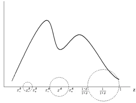
Notice that in (2.5) the amplitude of the technological neighborhood is propor-tional to the relative factor intensity of the country, that indexes its technological level: the more advanced the technology a country does operate, the larger the set of neighbouring technologies from which it can get useful knowledge (Figure 1). This assumption may seem strange at first: why a developed economy should be able to freely obtain useful knowledge over an inferior technology from a less developed one, while the latter cannot access the more advanced technology of the former?
The general idea is that an economy using a backward technology cannot sim-ply spill knowledge from a frontier technology without a costly investment, while an advanced technology often can integrate in its framework knowledge from an inferior technology (one can think of the case of the genetic improvement of crop varieties, often using traditional agricultural knowledge of local communities). This specification seems to be consistent with the empirical evidence discussed by Caselli (2005) and Feyrer (2003): there is a significant positive correlation of the produc-tivity residual A and measures of physical and human capital stock, so that the cross-country factor and TFP distributions seem to depend on each other. Equa-tion (2.5) has the potential to explain cross-country variaEqua-tion in both per capita income and TFP through cross-country variation in factor intensity: in the second part of this thesis we provide evidence supporting this specification.
The immediate consequence of the localisation of knowledge spillovers, coher-ent with the appropriate technology assumption, is that the marginal effect of an increase of a country capital intensity k now depends on the shape of the WFD distribution: by moving up along the distribution a country passes into a different technology neighborhood and the variation in the knowledge flow depends on the WFD densities at the extremes of its current neighborhood
A0t(k) = ⎧ ⎪ ⎪ ⎪ ⎪ ⎨ ⎪ ⎪ ⎪ ⎪ ⎩ β Kt ³ Gt St(k) ´1−β δα (z+) ht(z+) ≥ 0 k ∈ h kmin,kminδ i β Kt ³ Gt St(k) ´1−β£ δα (z+) ht(z+) − δα (z−) ht(z−)¤ k ∈ h kmin δ , Kt δ i −Kβt ³ Gt St(k) ´1−β δα (z−) ht(z−) ≤ 0 k ∈ h Kt δ , Kt i (2.6) where z+= δz and z−= δz.
Note that for countries that are sufficiently far from the boundary values of the support [kmin, Kt], i.e for k ∈
h kmin δ , Kt δ i
, the marginal effect of a factor intensity increase now depends on the shape of the WFD in the technological neighborhood in which the economy is located, i.e. on the values ht(z+) and ht(z−) , and on
the size of the technological neighborhood, as measured by the parameter δ : for certain WFD this effect and the elasticity can be positive, so that an increase of its capital intensity and a gain in rank along the WFD can improve the productivity of a country. On the other hand, for very low-k (high-k) countries the marginal effect on productivity of an increase in k is always positive (negative), since their technological neighborhood is left-truncated (right-truncated).
Backward knowledge spillovers can be introduced letting D = [kmin
Kt ,
k Kt] ≡
[zmin,z] so that the technology index becomes:
At(k) = St(k)βG1t−β ≡ ⎡ ⎢ ⎣1 + k/KZ t zmin α(z)ht(z)dz ⎤ ⎥ ⎦ β
G1t−β for all k ∈ [kmin, Kt]
(2.7) Here knowledge spillovers come from the sampling of the portion of the disti-bution of capital intensities indexing technologies already reached by the economy through costly investment: free informational leakage can only improve or upgrade existing production processes.
It is possible to interpret such a specification of the efficiency index also in terms of barriers to technology adoption, in the spirit of Parente and Prescott (1994): here low-k countries face a barrier that preclude them the access to the upper portion of the distribution of the world technologies, reducing their aggregate technological efficiency.
In this case the marginal effect of an increase in capital intensity is always positive A0t(k) = β Kt µ Gt St(k) ¶1−β
α (z) ht(z) ≥ 0 for all k ∈ [kmin, Kt] (2.8)
By raising its own aggregate capital intensity a country also increases accessed knowledge since it can extract useful knowledge from a greater part of ht(z). In
chapter 2 of this thesis we show that also (2.7) is consistent with empirical evidence.
Given (2.1), an increase in k through investment has a positive direct effect on a country per capita output but also an indirect effect, because it changes the component of a country’s resources it can freely borrow form other countries; in particular
Ft0(k) = A0t· k + At(k) = At(k) [1 + εt(k)] (2.9)
where εt(k) =A
0 t(k)·k
At(k) is the elasticity of the technology access function At(k),
which measures the percentage variation in productivity associated with a marginal increase in k: this elasticity is a crucial object in the following general equilibrium analysis, because an equilibrium WFD should equalize εt(k) among countries (from
(2.9) is also evident that εt(k) must be greater than -1, ensuring that the marginal
productivity of capital is not negative).
εt(k) = −βz
α (z) ht(z)
St(k)
(2.10) which measure the percentage loss associated with a one per cent increase in k: in this case (2.9) reveals that the production technology always display decreasing returns to scale for each country in the world economy, their degree varying with the shape of the WFD.
With appropriate technology spillovers one has
εt(k) = ⎧ ⎪ ⎪ ⎪ ⎨ ⎪ ⎪ ⎪ ⎩ βz St(k)zδα (z+) ht(z+) ≥ 0 k ∈ h kmin,kminδ i βz St(k) £ δα (z+) ht(z+) − δα (z−) ht(z−)¤ k ∈ h kmin δ , Kt δ i −Sβzt(k)δα (z−) ht(z−) ≤ 0 k ∈ h Kt δ , Kt i (2.11)
so that very low-k (high-k) countries always have increasing (decreasing) turns to scale, while for countries with complete technological neighborhoods re-turns to scale depend on the shape of the WFD and on the parameter δ which controls the size of the neighborhoods.
Finally with backward spillovers one has
εt(k) = βz
α (z) ht(z)
St(k)
(2.12) and the percentage gain associate to a marginal increase in k also measures the degree of increasing returns of each economy.
The presence of increasing returns to scale with appropriate technology and backward spillovers implies that a competitive equilibrium in general does not ex-ist: if k is paid its marginal productivity then Ft0(k) k = At(k) k [1 + εt(k)] >
At(k) k = Ft(k) and factor payments exceed the value of production. A
competi-tive equilibrium exists if, as in Romer (1986), in every country there exist a large number N of small firms so that aggregate capital intensity is given by the sum
k =
N
X
i=1
ki and the effect of an increase of the capital intensity of a sigle firm is
irrelevant: in this case every firm takes At as given while in the aggregate Atis
an increasing function of aggregate capital intensity k. Here we focus on optimal growth, that is on a world economy composed by countries whose factor accumu-lation trajectories are chosen by social planners that maximize total utility taking care of the externality associated with the presence of knowledge spillovers.
2.2. Optimal Growth of the World Economy. The economy faces convex
adjustment costs that are proportional to its output level, so that passing from k to ek in a unit time interval costs y · C³˜kk´ units of foregone consumption, where C0 > 0, C00 > 0 and the total capital stock depreciates at the constant rate η so that C (1 − η) = 0.
The social planner problem is that of maximizing total utility over an infinite horizon given the production technology (2.1): this is equivalent to maximizing net
production coherently with the representative agent’s preferences over consumption. Period t production net of adjustment costs is given byh1 − C³˜kk´iy, so that the PDV of national production of over the infinite horizon vt(k) solves
vt(k) = max ˜ k (" 1 − C Ã ˜ k k !# At(k) · k + 1 1 + rvt+1 ³ ˜ k´ ) (2.13)
where r is the exogenous world interest rate.
Using the first-order and envelope conditions as in Eeckhout-Jovanovic (2002), it is possible to obtain a second-order difference equation in k which characterizes the optimal factor accumulation path
(1 + r) C0 µk t+1 kt ¶ At(kt) = At+1(kt+1) ½k t+2 kt+1 C0 µk t+2 kt+1 ¶ + + ∙ 1 − C µ kt+2 kt+1 ¶¸ [1 + εt+1(kt+1)] ¾ (2.14)
then one can proceed in finding a solution in which every economy accumulates k at the same rate xk, so that ht(z) = h (z) holds and the cross-country factor
distribution is time-invariant, while total factor productivity grows only through the increase of common knowledge, xA≡AAt+1t = (1 + g)1−β from (2.2).
Now suppose that every economy shares the same preferences over consump-tion, that are characterized by a common CRRA utility function for the represen-tative consumer U = ∞ X t=0 ρtc 1−γ t − 1 1 − γ ρ < 1 γ > 0 (2.15)
where ρ is the subjective discount rate and γ controls the elasticity of intertem-poral substitution of consumption. Now it is possible to eliminate r from (2.14) using the FOC for consumption and the fact that the growth rate of consumption must equal the growth rate of potential output, or xc = xkxAfrom (2.1).
The crucial assumption of this general equilibrium analysis is
εt(k) = ε for all k and for all t (2.16)
An equilibrium WFD is such that the elasticity of the access function At(k) to
k is equalized among countries: if the percentage change associated with a marginal shift along the support of the WFD is completely independent of the position of the country along the WFD, then there is no incentive to change position and the factor distribution, and by consequence the world income distribution, is the equilibrium one.
If (2.16) holds, (2.14) reduces to an equation in the single variable xk = x
Ψ (x) ≡ h(ξx)γ ξρ − x i C0(x) 1 − C (x) = 1 + ε (2.17) where ξ = (1 + g)1−β.
We show in the Appendix that Ψ is a strictly increasing function, so that, given a value for ε, the common equilibrium growth rate of every economy is uniquely
determined, provided some restrictions on the cost function C (x) and the elasticity of marginal utility γ hold (in the Appendix we present also a detailed derivation of the optimization procedure).
Proposition 1
If the cost function verifies hγ[ξ(1−η)]ρ γ−1 − 1i(1−η)C
0
(1−η)
1−C(1−η) < 1 + ε and if γ > ξx
1+r then, for any ε > −1, there exist a unique growth rate x which solves (17),
where x ∈³1 − η, minhC−1(1),(1+r) ξ
i´
. Moreover, the equilibrium growth rate x is an increasing function of ε.
Proof. Appendix A. ¤
As an example, if adjustment costs are defined by the convex function C(x) = B [x − (1 − η)]θ, with B > 0 and θ > 1, and γ > 1 then an equilibrium always exists for any given ε > −1. The lower bound on the growth rate is given by the situation in which investments are null and the capital stock depreciates at the constant rate η, while the upper bound is given by the the two restrictions of the No-Ponzi game condition and of the non-negativity of net production.
Notice that:
• Since with forward spillovers model εt(k) is always negative, the
equlib-rium growth rate x∗
kis decreasing in the absolute value |ε| of this elasticity:
the greater the accessed knowledge loss associated with an increase in firm size, the larger the incentives to stay back and not accumulate capital for firms and the lower the steady-state growth rate.
• The no-externality case with β = 0 (which is just the standard Ak model) and the k-independent externality case of Romer (1986) or Lucas (1988) where At is equal to the mean of the distribution and the position of
the single country is irrelevant (∂At/∂k = 0), are characterized by the
condition ε = 0 and share the same growth rate, which is greater than with forward spillovers: moreover in both cases any initial distribution H0(z) simply replicates itself and can be sustained in a BGP equilibrium,
so that there is no restriction the theory can impose on the equilibrium WFD and WID.
• With appropriate spillovers ε can in principle be either positive or nega-tive, and the WFD and WID can be such that the world economy displays either decreasing or increasing returns to scale: in the next section we show that an equilibrium WFD with appropriate technology knowledge spillovers always induce constant returns to scale for the world economy. • With backward spillovers ε is always positive and the world economy always displays increasing returns to scale: moreover the growth rate of the world economy is an increasing function of the degree of increasing returns, which in turn depend on the equilibrium WFD.
In any case, the fundamental issue is the cross-country equalization of the elas-ticity εt(k) of the technolgy index which depend on the cross-country distribution
all possible type of knowledge spillovers, but the shape of the equilibrium WFD depends on the spillovers structure.
3. The Equilibrium World Income Distribution
3.1. The Equilibrium WID with Appropriate Technology Knowledge Spillovers. In the general framework given by (2.1) and (2.2) there are three el-ements which determine the shape of the equilibrium WFD: the copying function α (z), the strength of the spillovers as measured by the parameter β and the elas-ticity ε of the knowledge function At(k). The crucial element for a distribution to
be an equilibrium one is the equalization of εt(k) among countries, which could be
conjectured to be the outcome of the evolution of the world economy starting with an initial distribution of relative factor intensities/technological processes H0(z). In
the forward spilovers specification for At(k) the direction of the force represented
by this elasticity is the same for every country in the support, even if its magnitude can be different for each firm along its transition path: accumulating capital and gaining rank along the WFD reduces the quantity of accessed knowledge for every country in the support, so that the existence of spillovers always acts as an incentive to stay back (it is the "free-riding case", as Eeckhout and Jovanovic (1998) defined it in the working paper version of their paper).
In the appropriate technology framework, as it is specified in (2.5), the mar-ginal effect of an increase in capital intensity and the sign of the elasticity εt(k)
is ambiguous for countries sufficiently far from the boundary values of the support and opposite in direction for very low-k and very high-k countries as (2.11) shows: it is a boundary effect that pushes backward economies up along the WFD, since they always have a net positive effect by moving forward along the distribution, and pulls the advanced ones back because, being the technological leaders, they have no larger technological neighborhood to reach. The presence in the appropriate technology framework of these two opposite forces at the edges of the WFD support makes it difficult to find an equilibrium which is defined as
Definition 1
An equilbrium for the world economy described by (1), (5) and (15) consists of: - an elasticity ε > −1
- a growth rate x ∈³1 − η, minhC−1(1),(1+r) ξ
i´
- a lower bound zmin∈ [0, 1] of the support of the world factor distribution
- a world factor distribution, i.e. a function h (z) : [zmin, 1] → R that verifies 1
Z
zmin
h (z) dz = 1
such that (16) and (17) hold.
Since β > 0, α (z) and ht(z) are positive functions so that the integrand in
At(k) is always positive, equation (2.11) shows that a solution with ε > 0 cannot
exist because for k ∈ hKt
δ , Kt
i
have equality and the WFD coincide with a degenerate point mass centered in z = 1 and every country has the same factor intensity, the upper tail of the distribution always feels a force that pulls it back. It follows that in equilbrium ε ≤ 0.
Can an equilibrium with ε < 0 exist? It seems that at the lower tail of the WFD there is a symmetric problem, because for k ∈hkmin,kminδ
i
the elasticity is always positive. But as kmin gets smaller and smaller this part of the support shrinks and
the elasticity, as a measure of the force that pushes up backward countries, also becomes smaller and smaller. As kmin → 0 (2.11) is reduced to a system of two
equations βz St(k) £ δα (z+) ht(z+) − δα (z−) ht(z−) ¤ = −ε k ∈ µ 0,Kt δ ¸ (3.1) −Sβz t(k) δα(z−) ht(z−) = −ε k ∈ ∙ Kt δ , Kt ¸ (3.2)
and an equilibrium WFD with ε < 0 may exist.
In order to characterize the equilibrium WFD one can proceed in the same way as Eeckhout and Jovanovic (2002). Since (2.16) holds we have:
A0t(k) At(k)
= ε
k → At(k) = λtk
ε (3.3)
for some sequence of costants of integration {λt}.
Substituting from (2.5) gives:
G1t−β ⎡ ⎢ ⎣(1 + δ(k/KZ t) δ(k/Kt) α(z)h(z)dz) ⎤ ⎥ ⎦ β = λtkε k ∈ µ 0,Kt δ ¸ (3.4) and G1t−β ⎡ ⎢ ⎣(1 + 1 Z δ(k/Kt) α(z)h(z)dz) ⎤ ⎥ ⎦ β = λtkε k ∈ ∙ Kt δ , Kt ¸ (3.5)
and calculating the two sides of (3.4) and (3.5) for k = Kt
δ λt= µ Kt δ ¶−ε G1t−β ⎡ ⎢ ⎣1 + 1 Z δ/δ α(z)h(z)dz ⎤ ⎥ ⎦ β k ∈ (0, Kt] (3.6)
and eliminating λtfrom (3.4) and (3.5) leaves with an implicit characterization
1 + z+ Z z− α(z)h(z)dz =¡δz¢ ε β ⎡ ⎢ ⎣1 + 1 Z δ/δ α(z)h(z)dz ⎤ ⎥ ⎦ z ∈ µ 0, 1 1 + δ ¸ (3.7) 1 + 1 Z z− α(z)h(z)dz =¡δz¢ ε β ⎡ ⎢ ⎣1 + 1 Z δ/δ α(z)h(z)dz ⎤ ⎥ ⎦ z ∈ ∙ 1 1 + δ, 1 ¸ (3.8)
which can be rewritten as
[(1 + δ) z]εβ = ⎧ ⎪ ⎪ ⎪ ⎪ ⎪ ⎪ ⎪ ⎪ ⎪ ⎪ ⎪ ⎪ ⎨ ⎪ ⎪ ⎪ ⎪ ⎪ ⎪ ⎪ ⎪ ⎪ ⎪ ⎪ ⎪ ⎩ 1+ Z z+ z− α(z)h(z)dz 1+ Z 1 δ/δ α(z)h(z)dz z ∈³0,1+δ1 i 1+ Z 1 z α(z)h(z)dz 1+ Z 1 δ/δ α(z)h(z)dz z ∈h1+δ1 , 1 i (3.9)
But, while the left hand side of this equilibrium equation diverges as z → 0 since ε < 0, the right hand side of (3.9) is bounded. In the undirected copying hypothesis ( α(z) = α) since h(z) is a density function its integral over a subset of the support cannot be greater than 1 and the right hand side must be inh1+α1 , 1 + αi. If copying is directed the boundedness of the RHS of (3.9) follows from the fact that α(z) is bounded in [zmin, 1] .
It follows that an equilibrium CFD with ε < 0 is impossible, and the only possible equilibria in the appropriate technology framework are those with ε = 0: appropriate technology knowledge spillovers always entail an equilibrium world economy characterized by constant returns to scale.
Imposing the equilibrium condition ε = 0 greatly restricts the shape and prop-erties of the equilibrium distribution. Suppose that h(z) is an equilibrium WFD defined over [zmin, 1] ⊆ [0, 1]: once again, since β > 0, α (z) and h(z) are positive
functions and At(k) is always positive, by (2.11) the equilibrium condition ε = 0 is
verified at the boundaries of the support if and only if
h(z+) = 0 z ∈ [zmin, zmin 1 − δ] (3.10) h(z−) = 0 z ∈ [ 1 1 + δ, 1] (3.11) so that
h(z) = 0 z ∈ [(1 + δ)zmin,
(1 + δ)
(1 − δ)zmin] (3.12) h(z) = 0 z ∈ [(1 − δ)
(1 + δ), 1 − δ] (3.13)
For countries that have a complete technological neighborhood the equilibrium condition is in general (1 + δ) α (z+) ht(z+) = (1 − δ) α (z−) ht(z−) k ∈ ∙ kmin δ , Kt δ ¸ (3.14) so that in equilibrium ht(z+) = 0 ⇒ ht(z−) = 0 (3.15)
Since by definition z+= (1+δ)(1−δ)z− (3.10) and (3.11) imply also2
h(z) = 0 z ∈ [(1 + δ) 2 1 − δ zmin, µ 1 + δ 1 − δ ¶2 zmin] (3.16) h(z) = 0 z ∈ [ µ 1 − δ 1 + δ ¶2 ,(1 − δ) 2 1 + δ ] (3.17)
Iterating this passage one obtains
h (z) = 0 for ⎧ ⎨ ⎩ z ∈ Pn = [ (1+δ) n (1−δ)n−1zmin, ³ 1+δ 1−δ ´n zmin] z ∈ Qn= [ ³ 1−δ 1+δ ´n ,(1+δ)(1−δ)n−1n ] n ∈ N (3.18) so that Proposition 2
The set of the equilibrium world factor distibutions for the world economy de-scribed by (1), (5) and (15) consists of all distributions h(z) defined over
inter-vals [zmin, 1], for some zmin ∈ [0, 1], such that h(z) = 0 for z ∈
à [ n∈N Pn ! ∪ à [ n∈N Qn !
∩ [zmin, 1]. The associated equilibrium world income distribution is then
obtained through (1).
2One can reason along this line: (1+δ)z
min= z−for z =(1+δ)(1−δ)zmin, so that z+= (1+δ)
2
1−δ zmin
and since h [(1 + δ)zmin] = 0then (30) impose that also h
k
(1+δ)2 1−δ zmin
l = 0.
Thus, the set of equilibria for a world economy characterized by the presence of local spillovers or appropriate technology is very different from that of a world economy in which knowledge spillovers are global, either because of a common world technology assumption à la Solow or because the technology index depends on the average factor intensity à la Romer-Lucas: even if preferences over consumption are identical for each country, absolute convergence in relative factor intensity and income levels is not the only equilibrium outcome, as in Solow, but also not every cross-country factor distribution and world income distribution are equilibria, as in the Romer-Lucas framework.
Here convergence of the WFD and WID to a degenerate point mass and absolute convergence in relative income levels is indeed an equilibrium, but in general an equilibrium WFD, and the associated equilibrium WID, will not be continuous over its support and its density mass will be concentrated over disconnected intervals of [zmin, 1] : this can be interpreted as the equilibrium endogenous formation of
convergence clubs, where countries cluster toward different long run relative factor intensity, or relative technological levels, and the world economy is characterized by a permanent degree of inequality (Figure 2). In an appropriate technology framework where knowledge spillovers diffuse over a localized portion of the world capital intensity-technology distribution, an equilibrium distribution is attained by splitting the world economy in separate technological clusters between which there are no knowledge spillovers: in this sense, the observed bimodality of the WID could be interpreted as a sign of a long run tendence toward a split of the world economy in two distinct technological neighbourhoods. In each technological cluster every economy shares the same level of efficiency even if capital intensities differ: every technological cluster behaves as a Romer-Lucas economy in which every distribution of factor intensitiy is an equilibrium.
3.2. The Equilibrium WID with Backward Knowledge Spillovers. The definition of an equilibrium for a world economy characterized by the pres-ence of backward spillovers/barriers to technology adoption changes slightly, since in this case ε is always positive
Definition 2
An equilbrium for the world economy described by (1), (7) and (15) consists of: - an elasticity ε > 0
- a growth rate x ∈³1 − η, minhC−1(1),(1+r) ξ
i´
- a lower bound zmin∈ [0, 1] of the support of the world factor distribution
- a world factor distribution, i.e. a function h (z) : [zmin, 1] → R that verifies 1
Z
zmin
h (z) dz = 1
such that (16) and (17) hold.
Since (2.16) and (3.3) hold, for some sequence of costants of integration {λt} ,
G1t−β ⎡ ⎢ ⎣1 + k/KZ t zmin α(z)ht(z)dz ⎤ ⎥ ⎦ β
= λtkε for all k ∈ [kmin, Kt] (3.19)
and evaluating this identity at k = kmin one obtains
λt= G1t−βkmin−ε (3.20)
and it is now possible to eliminate λtfrom (3.19)
1 + k/KZ t zmin α(z)ht(z)dz = µ k kmin ¶ε β
for all k ∈ [kmin, Kt] (3.21)
Finally, noting that kmink = zminz and differentiating both sides with respect to z one obtains h(z) = ε βα(z)z ε β min z−(1−βε) (3.22)
that, together with the restriction that
1
Z
zmin
h (z) dz = 1, gives the equilibrium
WFD for any ε and any copying function α(z).
Suppose copying is undirected and α(z) = α (in the following we maintain this assumption). Then it is possible to obtain a closed form solution for the equilibrium WFD h(z) imposing the normalization:
1 Z zmin h(z)dz = ε βαz ε β min 1 Z zmin z−(1−βε) = 1 (3.23) from which zmin= µ 1 1 + α ¶β ε (3.24) and h(z) = ε(1 + α) βα z −(1−ε β) (3.25)
In this case the shape of the equilibrium WFD is controlled by the ratio ε β,
that is by the ratio between the degree of increasing returns of the world economy and the strength of knowledge spillovers: if spillovers are weak (ε
β > 1) then the
WFD is increasing and a large mass of the world economy is concentrated near the technological frontier, if spillovers are strong (ε
β < 1) then the WFD is decreasing
and the density mass of the world economy shifts toward the minimum zminof the
ε = βz αh (z)
[1 + αH(z)] (3.26)
then, given ε and for any relative factor intensity z, an increase of the strength β of spillovers must be offset by a decrease of the [1+αH(z)]αh(z) ratio: for any z either its density h (z) decreases or H(z), the density mass concentrated below z, increases.
Intuitevely, for a given ε, a high β amplifies the volume of accessed knowledge S, which is bigger near the technological frontier since high-z countries have access to a larger portion of the WFD: this effect is countered by a shift of the density mass of the equilibrium WFD toward the lower bound of the support zmin, which
in turn, as (3.24) shows, shifts back following an increase in β.
Proceding as in Eeckhout and Jovanovic (2002), we measure the impact of an increase in β on the dispersion of the equilibrium WFD as measured by the position of its percentile. Denoting with zp the value of z that identifies the percentile p of
the equilibrium distribution H(z), i.e. that solves
1 − p =
1
Z
zp
h(z)dz ≡ Φ(βε, zp) (3.27)
by the implicit function theorem ∂zp
∂ (ε/β) = − Φ1
Φ2 for all p ∈ [0, 1)
(3.28)
Since Φ2≡∂z∂Φp < 0, the sign of (3.28) depends on Φ1≡ ∂(ε/β)∂Φ . When copying
is undirected this is given by
Φ1≡ ∂Φ ∂w = ∂ ∂w ⎛ ⎜ ⎝(1 + α)α 1 Z zp wzw−1dz ⎞ ⎟ ⎠ = =(1 + α) α 1 Z zp zw−1dz + (1 + α) α 1 Z zp wzw−1ln zdz = = (1 + α) α 1 Z zp zw−1dz + (1 + α) α ⎛ ⎜ ⎝ 1 Z zp wzw−1ln zdz ⎞ ⎟ ⎠ = = (1 + α) α 1 Z zp zw−1dz + (1 + α) α ⎛ ⎜ ⎝[zwln z]1zp− 1 Z zp zw−1ln zdz ⎞ ⎟ ⎠ = = −(1 + α)α zpwln zp> 0 (3.29) since zp < 1.
It follows that, when copying is undirected, ∂zp
∂(ε/β) > 0 and cross-country
the degree ε of increasing returns of the world economy. Notice also that as spillovers dissapear the WFD converges to a degenerate point mass centered in z = 1, since
lim
β→0zm= 1. Since, by proposition 1, the higher ε the higher the equilibrium growth
rate of the world economy, there is also a clear relationship between growth and inequality over the WFD.
Proposition 3
When copying is undirected, an increase in the intensity of knowledge spillovers entails a rise in the dispersion the equilibrium WFD, since every percentile of the distribution is shifted back (∂zp
∂β < 0) and its support enlarges ( ∂zm
∂β < 0). As
spillovers disappear, convergence to a unique world factor intensity is obtained. An increase in the degree of the increasing returns and in the equilibrium growth rate of the world economy entails a reduction in the dispersion of the equilibrium WFD (∂zp
∂ε > 0) and shrinks its support ( ∂zm
∂ε > 0). Thus, growth and inequality
over the WFD are negatively related: the higher the equilibrium growth rate of the world economy the lesser the dispersion of the cross-country distribution of factor intensity.
This results shed a new light on those obtained by Eeckhout and Jovanovic (2002) for the forward spillovers version of the model and show that the inequality-augmenting effect of knowledge spillovers does not depend on their direction but on their mere existence: even an increase in the intensity of backward spillovers, that raises the incentive to gain rank along the relative factor intensity distribution and that could have been supposed to act as an equalizing force, entails a rise of the dispersion of the equilibrium WFD, needed in order to equalize εt(k) across
countries. Moreover with backward spillovers growth and inequality over the WFD are negatively related, while the reverse is true with forward spillovers since ε is always negative and a rise of its absolute value lowers the equilibrium growth rate of the world economy.
The final step consists in calculating the equilibrium distribution of productiv-ities and per capita incomes. In an equilibrium with undirected copying
At(k) = S(k)βG1t−β ≡ ⎡ ⎢ ⎣1 + α k/KZ t zmin h(z)dz ⎤ ⎥ ⎦ β G1t−β = [1 + αH(z)]βG1t−β (3.30)
and using (3.24) and (3.25)
H(z) = ε(1 + α) βα z Z [1/(1+α)]βε s−(1−βε)ds = (1 + α)z ε β − 1 α (3.31) so that At(k) = G1t−β(1 + α) β zε (3.32)
The world productivity distribution (WPD) shifts over time due to exoge-nous common technological change Gt, but the distribution of relative productivity
a(z) = At(z)/At(1) is time-invariant since
a(z) = zε (3.33)
where a is defined over [amin, 1] and amin= zεmin=
³
1 1+α
´β
.
Abusing notation and interpreting H(z) as the distribution function of a ran-dom variable, it is possible to calculate the distribution function HA(a) of relative
productivity in equilibrium noting that
HA(a) = Pr {a(z) ≤ a} = Pr {zε≤ a} = Pr n z ≤ a1ε o = = H(a1ε) = (1 + α)a 1 β − 1 α (3.34)
that implies the density
hA(a) = H 0 A(a) = (1 + α)aβ1−1 βα a ∈ "µ 1 1 + α ¶β , 1 # (3.35)
Notice that, when copying is undirected and total knowledge spillovers are proportional to H(z), the equilibrium distribution of relative productivity does not depend on the elasticity ε but only on the constant α and on the intensity β of spillovers: since an equilibrium WFD equalizes ε across countries in order to eliminate incentives for a country to change its own relative factor intensity to raise the amount of accessed knowledge, a variation in ε entails a direct effect on the WFD, as Proposition 3 shows, which neutralizes its effect on the world productivity distribution (WPD).
Proceding as in the case of the equilibrium WFD, the dispersion of the WPD can be shown to be increasing in the intensity of knowledge spillovers.
Proposition 4
When copying is undirected, an increase in the intensity of knowledge spillovers entails a rise in the dispersion the equilibrium WPD, since every percentile of the distribution is shifted back (∂ap
∂β < 0) and its support enlarges ( ∂am
∂β < 0). An
increase in the degree of the increasing returns and in the equilibrium growth rate of the world economy has no effect on the equilibrium WPD.
Per capita income relative to the technological leader, yr ≡ AAt(Kt(k)t)·k·Kt = a(z)z
is given in equilibrium by:
yr= z1+ε (3.36) where yr∈£yminr , 1 ¤ and ymin r = z1+εmin = ³ 1 1+α ´β(1+ε) ε .
The equilibrium world income distribution is a transformation of the WFD that can be explictely derived proceding as in the case of the WPD, obtaining the density
hY(yr)= εα β(1 + ε)(1 + α)y ε β(1+ε)−1 r yr∈ ⎡ ⎣µ 1 1 + α ¶β(1+ε) ε , 1 ⎤ ⎦ (3.37)
We measure inequality over the WID with the percentile approach applied above. Denoting with yp
r the p-percentile of the equilibrium distribution of relative
income and proceding as in the WFD case
∂ypr ∂³ ε
β(1+ε)
´ > 0 for all p ∈ [0, 1) (3.38)
and noting that d dε
³
ε β(1+ε)
´
> 0, one obtain the following relationship between spillovers, growth and dispersion of the long run WID.
Proposition 5
When copying is undirected, an increase in the intensity of knowledge spillovers entails a rise in the dispersion the equilibrium WID, since every percentile of the distribution is shifted back (∂ypr
∂β < 0) and its support enlarges ( ∂yrmin
∂β < 0). As
spillovers disappear, absolute convergence to a unique relative per capita income is obtained. An increase in the degree of the increasing returns and in the equilibrium growth rate of the world economy entails a reduction in the dispersion of the equi-librium WFD (∂yrp
∂ε > 0) and shrinks its support ( ∂ymin
r
∂ε > 0). Thus, growth and
inequality over the WID are negatively related: the higher the equilibrium growth rate of the world economy the lesser the dispersion of the cross-country distribution of per capita income.
Thus the existence of spillovers at the same time accelerates growth of the world economy, inducing increasing returns to scale and, and creates a dispersion of long-run per capita income that otherwise would have not existed. On the other hand, the rate of growth of the world economy in equilibrium is negatively correlated with the dispersion of the WFD and the WID: the more concentrated the distribution of factor intensity, intuitevely representing a situation in which many countries of the world economy operate similar technologies, the higher the elasticity of accessed knowledge, the degree of increasing returns and the growth rate. This seems to be consistent with empirical evidence documented by Sala-i-Martin (2006) on the reduction of various measures of inequality for the world income distribution over the period 1970-2000: in the same period the growth rate of the world economy has continously increased.
4. Conclusion
We introduced a specification of the technology index in which knowledge spillovers can be either localized, coherently with the appropriate technology hy-pothesis, or backward directed, coherently with either the upgrading technology assumption or with the existence of barriers to technology adoption linked to rel-ative factor intensity. With appropriate technology, knowledge spillovers between countries are likely to be localized, since only neighbouring technologies provide use-ful information that can be shared. As a consequence, the spillovers force depends on the local shape of the cross-country capital intensity distribution that, since total factor intensity is also an index of the technological state of an economy, can also be interpreted as the cross-country technology distribution, and the dynamics of the world income distribution now depends on the strenght of these spillovers. The resulting set of equilibria for a world economy characterized by appropriate tech-nology and local spillovers is very different from that of the Solow model, with a common world technology assumption, and that of the Lucas-Romer type, in which spillovers are measured by average total capital intensity: even if every country of the world economy shares the same preferences over the intertemporal consumption allocation, absolute convergence is not the only equlibrium outcome as in Solow, nor any WID is an equilibrium as in the Lucas-Romer specification. In general, even if convergence to a degenerate point mass distribution is an equilibrium, any cross-country technology distribution that clusters the world economy into long-run relative technology levels between which there are no spillovers is an equilibrium: thus the model provides an explanation for the emergence of convergence clubs, as a result of the localization of the spillovers force.
With backward knowledge spillovers the equilibrium WFD and WID depend on the strength of spillovers and on the degree of increasing returns attained in equilibrium by the world economy, which in turn depends on the dispersion of the WFD. Given the degree of increasing returns, an increase in the intensity of the spillover force raises inequality over the WFD and the WID to equalize returns to scale in the world economy. Given the intensity of spillovers, a less dispersed WFD in which many countries are near the technological frontier induce an acceleration in the growth rate of the world economy: in equilibrium growth and inequality are negatively related.
5. References
Aghion, P. and Howitt, P. (1998), Endogenous Growth Theory, MIT Press, Cambridge (MA).
Atkinson, A.B. and Stiglitz, J. (1969), "A New View of Technological Change", Economic Journal, LXXIX, 573-578.
Basu, S. and Weil, D. (1998), “Appropriate Technology and Growth”, Quarterly Journal of Economics, 113(4), 1025—54.
Beine, M., Docquier, F. and Rapoport, H. (2001), “Brain Drain and Economic Growth: Theory and Evidence”, Journal of Development Economics, 64(1), 275-289.
Boldrin, M. and Levine, D. (2005), "The Economics of Ideas and Intellectual Property", Proceedings of the National Academy of Sciences, 102 , 1252-1256.
Caselli, F. (2005), “Accounting for Cross-Country Income Differences”, Hand-book of Economic Growth vol. 1 (Aghion,P. and Durlauf, S. eds.), North-Holland. Docquier, F. and Marfouk, A. (2006), “International Migration by Educational Attainment, 1990-2000”, International Migration, Remittances, and the Brain Drain ( Ozden, C. and Schiff, M. eds.), Washington, DC: The World Bank and Palgrave McMillan, pp. 151-200.
Eeckhout, J. and Jovanovic, B. (1998), "Inequality", NBER Working Paper n. 6841.
Eeckhout, J. and Jovanovic, B. (2002), "Knowledge Spillovers and Inequality", American Economic Review, 92(5), 1290-1307.
Feyrer, J. (2003), "Convergence by Parts", mimeo, Dartmouth College. The Economist (2006), "Starbucks vs Ethiopia. Storm in a coffee cup", No-vember 16 .
Gerschenkron, A. (1962), Economic Backwardness in Historical Perspective, Harvard University Press, Cambridge (MA).
Hall, R. and Jones, C. (1999), "Why Do Some Countries Produce So Much More Output per Worker Than Others ?", Quarterly Journal of Economics, 114(1), 83-116.
Lucas, R. (1988), "On the Mechanics of Economic Development", Journal of Monetary Economics, 22(1), 3-42.
Lucas, R. (2001) "Some Macroeconomics for the 21st century", Journal of Economic Perspectives, 14(1),159-168.
Mankiw,N., Romer, D. and Weil, D. (1992), "A Contribution to the Empirics of Economic Growth", Quarterly Journal Of Economics 107, 407-437.
Parente, S. and Prescott, E. (1994), "Barriers to Technology Adoption and Development," Journal of Political Economy, 102 (2), 298-321.
Quah, D. (1997), "Empirics for Growth and Distribution: Polarization, Strat-ifcation, and Convergence Clubs", Journal of Economic Growth 2(1) 27-59.
Romer, P. (1986), "Increasing Returns and Long Time Growth", Journal of Political Economy, 94(5), 1002-1037.
Sala-i-Martin, X. (2006), "The World Distribution of Income: Falling Poverty and. . . Convergence, Period", Quarterly Journal of Economics, 121 (2), 351-397.
Seager, A. (2006), "Starbucks, the coffee beans and the copyright row that cost Ethiopia £47m", The Guardian, October 26.
Young, A. (1995), “The Tyranny of Numbers: Confronting the Statistical Real-ities of the East Asian Growth Experience”, Quarterly Journal of Economics, 110, 641-680.
Young, A. (2003), “Gold into Base Metals: Productivity Growth in the People’s Republic of China during the Reform Period”, Journal of Political Economy, 111, 1220-1261.
Existence and Uniqueness of the Equilibrium
We have shown in the text that the economy optimal capital accumulation path chosen by the social planner over the infinite horizon must solve the functional equation vt(k) = max ˜ k (" 1 − C Ã ˜ k k !# At(k) · k + 1 1 + rvt+1 ³ ˜ k´ ) (A1)
We proceed as in Eeckhout and Jovanovic (2002), starting with the first-order and envelope conditions:
C0 Ã ˜ k k ! At(k) = 1 1 + rv 0 t+1 ³ ˜ k´ (A2) v0t(k) = " 1 − C Ã ˜ k k !# At(k) + " 1 − C Ã ˜ k k !# A0t(k) · k + C0 Ã ˜ k k ! ˜ k kAt(k) = At(k) " ˜ k kC 0 + (1 − C) [1 + εt(k)] # (A3) where εt(k) = A 0 t(k)·k
At(k) is the elasticity of the technology access function At(k) .
Uptading one period the envelope condition (A3) and substituting in (A2) gives the second order difference equation:
(1 + r) C0 µ kt+1 kt ¶ At(kt) = At+1(kt+1) ½ kt+2 kt+1 C0 µ kt+2 kt+1 ¶ + + ∙ 1 − C µ kt+2 kt+1 ¶¸ [1 + εt+1(kt+1)] ¾ (A4) that characterizes optimal investment.
In a world equilibrium every country accumulates total capital at the same gross rate kt+1
kt = x for each t, so that the cross-country factor distribution is
time-invariant, i.e. Ht(z) = H(z), and total factor productivity grows only through the
exogenous increase in common knowledge
xA≡
At+1
At
= (1 + g)1−β= ξ (A5)
Suppose also that H(z) is such that the elasticity of efficiency to capital is a constant:
εt(k) = ε for all k and for all t (A6)
Then (A4) becomes ∙
(1 + r)
ξ − x
¸
C0(x) = [1 − C (x)] (1 + ε) (A7) Denoting with xc ≡ ct+1ct the gross growth rate of consumption, the FOC for
optimal consumption, using the CRRA utility function (11), is
(1 + r) = x
γ c
ρ (A8)
Since consumption grows at the same rate of potential output, in such an equilibrium we have xc= xAx = ξx and it is possible to eliminate the interest rate
factor (1 + r) from (A6) to get an expression in the two unknowns x and ε
Ψ(x) ≡ h(ξx)γ ξρ − x i C0(x) 1 − C (x) = 1 + ε (A9)
Given ε, which is not determined explicitely in the model but that should be tought as the outcome of the dynamics of the CFD starting from an initial distribution H0(z) of relative factor intensities, an equilibrium is reached when
Ψ(x) = 1 + ε (A10)
holds.
We now show that, provided some restrictions on the cost function C and on the elasticity of marginal utility to consumption γ are verified, the equilibrium exist and is unique.
The first derivative of Ψ(x) with respect to x is
Ψ0(x) = " γ (ξx)γ−1 ρ − 1 # C0(x) 1 − C (x)+ (A11) + " (ξx)γ−1 ρ − 1 # x C00(x) [1 − C (x)] +hC0(x)i2 [1 − C (x)]2
Equation (A1) shows that 1 − C (x) > 0 , otherwise the firm would sustain net losses. In an equlibrium the consumption growth rate must not exceed the interest rate, xc < (1 + r), so that (ξx) γ−1 ρ = (ξx)γ ρξx = xγ c ρxc = (1+r)
xc > 1 and the second term
of the RHS of (A11) is positive. It follows that if
γ > xc 1 + r=
ξx
1 + r (A12)
then also the first term of the RHS of (A11) is positive, Ψ0(x) > 0 and the equation Ψ(x) = 1 + ε has a unique solution for any given value of ε.
The lowest possible growth rate of total capital x is that associated with a null investment: since the depreciation rate is η, x must be greater than 1 − η (notice that in this case the capital stock shrinks to zero in the long run). Then, for any given value of ε, for a solution to (A10) to exist the cost function C(x) must verify
" γ [ξ (1 − η)]γ−1 ρ − 1 # (1 − η) C0(1 − η) 1 − C (1 − η) < 1 + ε (A13) Since C(x) is an increasing and convex function, there will be also a growth rate x∗ for which C(x∗) = 1 : then, since C is invertible, x∗= C−1(1) is the maximum
sustainable equilibrium growth rate of total capital stock k , since for x > x∗ the
firm sustains net losses all over its infinite horizon. Notice that
lim
x→x∗Ψ(x) = ∞ (A14)
so that x∗ is reached only if ε → ∞ (Figure 3).
The other upper bound for the equilibrium growth rate is given by the No-ponzi game condition xc < (1 + r), that restrict x to be lower than (1+r)ξ so that
x ∈³1 − η, minhx∗,(1+r) ξ
i´ .
A possible specification for the cost function C(x) is
C(x) = B [x − (1 − η)]θ B > 0, θ > 1 (A15) where C(1 − η) = 0, i.e. there is no cost associated with a null investment, and C0(1 − η) = 0 so that (A13) holds for any ε > −1. In this case the maximum sustainable equilibrium growth rate of total capital stock k is given by x∗= B−1θ+
Figure 2. Equilibrium World Income Distribution with Appro-priate Technology Spillovers