Deep Question Answering: A New Teacher For DistilBERT

(1)

Alma Mater Studiorum · Universit`

a di Bologna

SCUOLA DI SCIENZE

Corso di Laurea Magistrale in Informatica

Deep Question Answering:

A New Teacher For

DistilBERT

Relatore:

Chiar.mo Prof.

Fabio Tamburini

Correlatore:

Chiar.mo Prof.

Philipp Cimiano

Presentata da:

Simone Preite

Sessione III

Anno Accademico 2018/2019

(2)

(3)

(4)

(5)

Sommario

Nel vasto ambito del Natural Language Processing (NLP), letteralmente tradotto come elaborazione del linguaggio naturale, sono stati proposti, nel corso del tempo, diversi modelli e tecnologie utili ad aggiungere questa ca-pacit`a ai calcolatori.

Lungo questo lavoro andremo ad esplorare quali sono gli strumenti disponi-bili oggigiorno, nello specifico vedremo i Transformer utilizzati all’interno del modello BERT [9], creato da Google, e di alcuni modelli derivati da esso. Questo modello `e al momento lo “stato dell’arte” per diversi problemi di NLP.

Andremo, in questa tesi, a focalizzarci sul Question Answering (QA), ovvero l’abilità di cercare automaticamente risposte a domande poste in lin-guaggio naturale. Il dataset di riferimento sarà SQuAD v2 ma verrà presen-tato anche un ulteriore dataset sperimentale di nome OLP, entrambi verranno successivamente descritti nel capitolo 4.

Il principale obiettivo di questo lavoro di tesi era quello di sperimentare i benifici ottenibili intervenendo sul livello di question answering. Ci si è ispi-rati al lavoro prodotto dal gruppo di ricerca HuggingFace ed al modello Distil-BERT in particolare. Questo modello utilizza il paradigma Teacher-Student (Insegnante-Studente) per trasmettere la capacità di generalizzazione tra due modelli (verrà spiegato in maggior dettaglio nella sezione 5.2.1) e promette di preservare il 97% della conoscenza di BERT, usato come Teacher dal gruppo di ricerca, ma riducendo considerevolmente le dimensioni ed aumentando in velocità di training ed inferenza.

(6)

ii Sommario

Infine verranno presentati i risultati ottenuti e spiegati i miglioramenti che, seppur modesti, risultano in una conservazione della conoscenza del 94% rispetto al Teacher utilizzato. A livello di modelli sia per lo Student che per il Teacher verranno proposti livelli di question answering modificati che vedremo nel relativo capitolo (6). Inoltre saranno comparati anche risultati ottenuti su OLP in diverse configurazioni con lo scopo di dimostrare come un modello come BERT possa essere messo in difficolt`a quando non si lavora con un ambiente che rispetta certi vincoli.

(7)

iv Table of Contents 3.1.4 Layer Normalization . . . 18 3.2 BERT . . . 20 3.3 Transfer Learning . . . 21 3.3.1 Pre-Training . . . 22 3.3.2 Fine-Tuning . . . 24 3.4 Derived Models . . . 26 3.4.1 RoBERTa . . . 26 3.4.2 ALBERT . . . 28 3.4.3 DistilBERT . . . 31 4 Question Answering 33 4.1 Question Answering Problem . . . 33

4.2 Datasets . . . 35 4.2.1 SQuAD v1.1 . . . 35 4.2.2 SQuAD v2 . . . 35 4.2.3 OLP Dataset . . . 36 4.3 Metrics . . . 38 4.4 Before BERT . . . 39 4.4.1 BiDAF . . . 39 4.4.2 ELMo . . . 40 4.5 Results Comparison . . . 41 5 DistilBERT 43 5.1 Models Compression . . . 43 5.1.1 Pruning . . . 43 5.1.2 Quantization . . . 44 5.1.3 Regularization . . . 44 5.2 Knowledge Distillation . . . 44 5.2.1 Teacher-Student . . . 45 5.2.2 Softmax-Temperature . . . 46 5.2.3 Dark Knowledge . . . 47 5.3 DistilBERT Model . . . 47

(9)

Table of Contents v 6 QADistilBERT 51 6.1 QABERT . . . 51 6.1.1 QABERT Vanilla . . . 51 6.1.2 QABERT 2L . . . 52 6.1.3 QABERT 4L . . . 54 6.2 Implementation . . . 55 6.3 Results . . . 57 6.4 SQuAD Results . . . 58 6.5 OLP Results . . . 60 Conclusion 63 6.6 Future Works . . . 64 A SQuAD examples 65 A.1 SQuAD v1.1 . . . 65 A.2 SQuAD v2 . . . 67 B OLP Dataset 69 B.1 OLP Article . . . 69 B.2 OLP Questions . . . 70 B.3 OLP Annotations . . . 71 C Training Summary 73 C.1 Configuration . . . 73 C.2 DistilBERT . . . 74 C.3 QADistilBERT4LGELUSkip . . . 77

D Question Answering Models 81 D.1 QABERT4LGELUSkip . . . 81

D.2 QADistilBERT4LGELUSkip . . . 84

(10)

(11)

List of Figures

1.1 NLP . . . 3

2.1 Artificial Neuron . . . 6

2.2 Single and Multilayer Perceptron . . . 7

2.3 CNN . . . 8

2.4 RNN . . . 9

2.5 Encoder-Decoder RNN . . . 10

2.6 CBOW and Skip-Gram . . . 12

3.1 Encoder-Decoder Attention . . . 13

3.2 Encoder-Decoder Attention . . . 15

3.3 Scaled Dot-Product . . . 16

3.4 Multi-Head Attention . . . 17

3.5 Multi-Head in Transformers . . . 18

3.6 Batch Normalization vs Layer Normalization . . . 19

3.7 BERT . . . 20 3.8 NSP Structure . . . 22 3.9 MLM Structure . . . 23 3.10 NSP Structure . . . 24 3.11 BERT fine-tuning . . . 26 4.1 QA architecture . . . 34 4.2 BiDAF . . . 40 4.3 ELMo . . . 41 vii

(12)

viii List of Figures

5.1 Teacher-Student Model . . . 46

6.1 QABERTVanilla model schema . . . 52

6.2 QABERT2LTanh model schema . . . 52

6.3 QABERT2LGELU model schema . . . 53

6.4 QABERT2LReLU model schema . . . 53

6.5 QABERT4LReLU model schema . . . 54

6.6 QABERT4LGELUSkip model schema . . . 55

B.1 OLP article . . . 69

B.2 OLP Questions . . . 70

B.3 OLP Annotations . . . 71

C.1 TensorBoard config1 DistilBERT . . . 74

C.7 TensorBoard config1 QADistilBERT4LGELUSkip . . . 77

(13)

List of Tables

3.1 Batch Normalization vs Layer Normalization . . . 19

3.2 Bert Dimensions . . . 21

3.3 RoBERTa vs BERT on SQuAD . . . 28

3.4 ALBERT dimensions . . . 30

3.5 ALBERT on SQuAD . . . 31

4.1 QA results summarize . . . 41

5.1 DistilBERT understanding . . . 49

5.2 DistilBERT understanding preservation . . . 49

5.3 DistilBERT smallness . . . 50

6.1 QABERT4LGELUSkip vs BERT-base-uncased . . . 58

6.2 Hyperparamenters Configurations . . . 59

6.3 Final Results . . . 60

6.4 Evaluation on OLP . . . 60

6.5 Fine-Tuning and Evaluation on OLP . . . 61

(14)

(15)

Listings

5.1 Fine-Tuning Loss . . . 48

5.2 Distillation Loss . . . 48

6.1 Vanilla BERT QA layer . . . 55

6.2 Vanilla BERT QA output . . . 56

6.3 QADistilBERT4LGELUSkip 4 layers . . . 56 6.4 QADistilBERT4LGELUSkip output . . . 56 A.1 Squad v1.1 . . . 65 A.2 Squad v2 . . . 67 D.1 QABERT4LGELUSkip . . . 81 D.2 QADistilBERT4LGEkLUSkip . . . 84 xi

(16)

(17)

Chapter 1 Introduction

In the few last years, the Natural Language Processing (NLP) field has seen a great expansion, also on large scale distribution. With the last technologies, understanding and processing human language became an im-portant part in research, making computer and other devices more human friendly.

Nowadays, we all have already used, at least once, systems like Amazon ALEXA, Google Home or Apple Siri. This is only a part of this field, which is composed by many other sub-fields like speech recognition, text generation and speech generation, text or natural language understanding. NLP plays an important role also as a baseline to create support devices for people with diseases, starting from a simple screen reader to a more complex kind of information retrieval.

We found the purpose of our studies in text comprehension and focused on the specific part of question answering by using the BERT model, which is State-of-the-Art at the moment for many NLP tasks. In the next section we will see an overview on what Natural Language Processing mean.

(18)

2 1. Introduction

1.1 Natural Language Processing

In short, the aim of this artificial intelligence field is to intermediate com-munication between humans and machines by using the natural language. Let us see some definitions (you can find them online) which explain the concept with better words.

Natural Language Processing, usually shortened as NLP, is a branch of arti-ficial intelligence that deals with the interaction between computers and hu-mans using the natural language. The ultimate objective of NLP is to read, decipher, understand, and make sense of the human languages in a manner that is valuable. Most NLP techniques rely on machine learning to derive meaning from human languages.1

Natural Language Processing (NLP) is a subfield of linguistics, computer sci-ence, information engineering, and artificial intelligence concerned with the interactions between computers and human (natural) languages, in particular how to program computers to process and analyze large amounts of natural language data.2

Natural Language Processing (NLP) is a branch of artificial intelligence that helps computers understand, interpret and manipulate human language. NLP draws from many disciplines, including computer science and computational linguistics, in its pursuit to fill the gap between human communication and computer understanding.3

NLP can be divided in four macroareas:

• Syntax 1_{https://becominghuman.ai/a-simple-introduction-to-natural-language-processing-ea66a1747b32} 2 https://en.wikipedia.org/wiki/Natural_language_processing 3_{https://www.sas.com/en_us/insights/analytics/what-is-natural-language-processing-nlp.} html

(19)

1.1 Natural Language Processing 3

• Semantics • Discourse • Speech

Of course, all of these areas have many subtasks like speech recognition, part-of-speech tagging, automatic summarization etc.

Ambiguity is one of NLP keywords. The ambiguity of natural languages makes all of the NLP tasks really challenging. We will focus on Question answering, which is part of the Semantics macroarea.

(20)

(21)

Chapter 2 Neural Networks

2.1 Artificial Neural Networks

An Artificial Neural Network, in the Machine Learning field, is an ar-tificial model composed of connected neurons which should reproduce a biological neural network. In other words, the Artificial Neural Network idea is directly inspired by the human brain structure. These networks are rep-resented by algorithms and they recognize numerical patterns, so we need to convert sensory data information into numerical representations before feeding them to the neural network.

Like signals transmitted through synapses, real numbers are transmitted among neurons through the connection of the artificial network. We will see the neuron and its possible activation functions more in details in the next sections.

2.1.1 Neuron

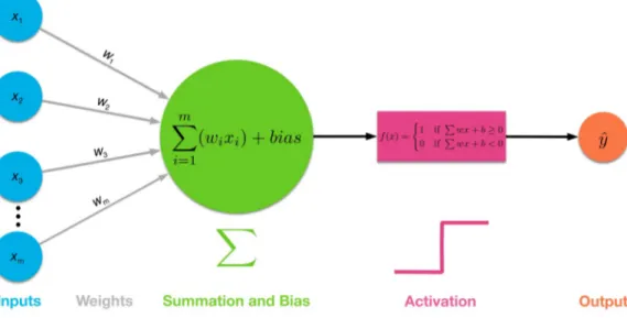
The neuron is the fundamental part of an Artificial Neural Network. This component receives a signal (a real number) input, makes some computation and sends its output to the other neurons. A neuron can receive more than one input at the same time; it processes all these signals to produce an unique output. Normally it sums all the inputs xiwi, where xi is produced by the

(22)

6 2. Neural Networks

i-th neuron and wi is the weight associated to the connection, and adds a

bias (if it exists) before feeding the result to the activation function.

Figure 2.1: Artificial Neron

2.1.2 Activation Functions

An Activation Function represents the final elaboration step of the neuron and it is performed before sending the output to other neurons.

Nowadays, the most popular function is the Rectified Linear Unit, also called ReLU [2], which allows a faster convergence. Other examples of acti-vation functions are the sigmoid and the tanh, defined as:

sigmoid(x) = 1

1 + e−x (2.1)

T anh(x) = 1 − e

−2x

1 + e−2x (2.2)

while the ReLU is simply defined as:

ReLU (x) = max(0, x) (2.3)

ReLU is fast to compute since its value is equal to the identity and 0 for all the negative x, so it is faster both during training and at inference time.

(23)

2.2 Type of ANN 7

In the next chapters, while talking about BERT, we will see the GELU [14] activation function used inside BERT by the Google AI research group. This function is defined as xP (X ≤ x) = xφ(x) which can be approximated to: GELU (x) = 0.5x[1 + T anh( r 2 π[x + 0.044715x 3_])] _(2.4)

This variant should preserve neurons from dying, since the negative values try to mitigate this case without eliminating it totally.

2.2 Type of ANN

2.2.1 Feed-Forward Neural Networks

The Feed-Forward Neural Network (FNN) [4] is an Artificial Neural Net-works that does not present loops. It is the first simplest model of ANN in which the information goes only forward, starting from the input nodes to the output ones and passing though the so called Hidden Layers.

The most simple example of a Feed-Forward network is the Simple Per-ceptron, composed only of the input and the output layers. Its neurons are fully connected between the two layers while the Multi-Layer Perceptron is composed of at least two layers of neurons without considering the input one instead. This generalization allows neural networks to represent and approximate complex non-linear functions.

(24)

2.2.2 Convolutional Neural Networks

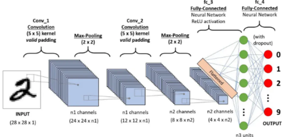
The Convolutional Neural Network (CNN) [24] is a special case of Multi-Layer Perceptron inspired by biological processes. This tries to represent the brain visual cortex. A CNN is composed of one or more Convolutional Layer and could also have some pooling layers and finally a linear fully connected network.

A Convolutional Layer extracts the features from an image. It acts similarly to a scanner moving a particularly small matrix, called kernel, over the entire image. Each convolutional layer extracts different kinds of features because these matrices act like filters. A convolution is a kind of parameter sharing, since each filter extracts the presence or the absence of a feature in an image, which is a function of not just one pixel but also of its surrounding neighbor pixels.

A Pooling Layer is normally applied after a series of Convolutional Lay-ers in order to downsample the input by reducing its dimension but preserving the features’ information.

The last level is composed of one or more Fully Connected Layers and its result is a dot product between the output of the previous layer and the weights’ matrix, which has to be trained.

(25)

2.2 Type of ANN 9

2.2.3 Recurrent Neural Networks

The keyword of the Recurrent Neural Network (RNN) [35] is memory. What does it mean? It means that, unlike a basic Feed-Forward Network, RNN remember things not only from the current training, but also maintain some context from previous inputs, the so called Hidden State Vectors. For example, the same input can produce different outputs, it depends on the previous inputs. In other words, a permutation of the input sequence normally leads to producing different outputs.

This kind of network is particularly suitable for tasks that need the help of a context, such as speech recognition and other Natural Language Processing tasks.

Parameter Sharing

RNN shares parameters across inputs. When this kind of network do not share them, it is only a normal FNN where each input has its own weights. The most commonly cells used in RNN are GRU [8] and the Long Short-Term Memory (LSTM) [37].

Figure 2.4: Simple representation of a Recurrent Neural Network

Encoder-Decoder Sequence to Sequence RNN

For translation services, this network is composed of two Recurrent Neural Network, the Encoder and the Decoder. The first one produces the context

(26)

output, the encoder vector that is fed to the decoder part which translates it to a sequence of outputs.

Figure 2.5: Encoder-Decoder with Recurrent Neural Network

2.3 Training

2.3.1 Hebb’s Rule

“Cells that fire togheter, wire together”, this is a summarize of the Donald Hebb’s postulate. It is not completely correct because the original postulate says “A cell A takes part in the activation of the cell B”[15], where A and B are two connected neurons. The weights are updated during the training phase at every training example, for a graphic representation have a look to the Picture 2.1.

The Hebb’s rule is obsolete and does not accurately describe the behaviour of a human brain. In fact, it assumes that a connection has to be strengthened independently whether the result is good or not.

(27)

2.4 Word Embedding 11

2.3.2 Backpropagation

Nowadays, Backpropagation [32] is used, which is a supervised learning technique that consists in minimizing the loss function by calculating the gradient (descent in case of minimizing, ascent instead).

The gradient is the multi-variable generalization of a derivative of a func-tion and determines how a weight value has to change and whether the corresponding connection has to be reinforced or not. The two main reasons to calculate the gradient are the following ones: the derivative shows the direction of the cost function and also how much the weight needs to change to minimize that function. After an input goes through a neural network, we calculate the gradients and the new weight, which are pushed back in the neural network to update all the weights inside it.

Although the gradient descent gives good results when changing weights, it is really slow and this reflects negatively on the training time, so we need to use some optimizers such as Stochastic Gradient Descent (sgd) [42] and Adam [19]

2.4 Word Embedding

The Word Embedding is a kind of document representation in the Natural Language Process field. It could be seen as a learning technique in which the words are translated in their real number vector representation, so they can conserve and give information about the context and the semantic for each word in a document. We need this representation because our aim is to capture word dependencies to reinforce the concept of context and have better information about word relations in a text.

One of the most famous technique which implements this idea is word2vec [26]. It uses Neural Networks and either Common Bag of Words (CBOW) or Skip-Gram [27]. The first one predict the word based on the context while the second one predicts the surrounding words given the current word.

(28)

Figure 2.6: Comparison between CBOW and Skip-Gram

2.5 Dropout

The overfitting problem in Neural Networks consists of a model unable to generalize, for example because it can become too specific about the training set. This means that the model will make good predictions on data seen during the training, but it will have bad performances when applying what it learnt to unknown data.

This problem is mitigated though normalization techniques such as Dropout [36]. It basically ignores randomly some connections by “dropping” them temporarily and by avoiding to correct mistakes from previous layers. This situation is called co-adaptation and could lead to overfitting because the network does not generalize on unknown data.

(29)

Chapter 3 Transformers

3.1 Transformers Architecture

Transformers is the actual State-of-the-Art in NLP introduced by the “Attention is all you need” paper [39]. A transformer is usually composed of two parts: the Encoder and the Decoder. Both of them have an Attention mechanism inside. Let us show in a more detailed way, in the next sections, the Encoder and the Decoder.

Figure 3.1: Transformers high-level structure

(30)

14 3. Transformers

3.1.1 Encoder

If we explode the Encoder and look inside it we will actually find many Encoders, going deeply in each of these “layers”, which have the same struc-ture. We will find a Multi-Head Attention layer with a normalization layer above and a Feed-Forward Network (a two layers network with ReLU ac-tivation function in between them) with another step of normalization on the top. The input goes through all the Encoder layers and at the end the final output is passed to each Decoder layer at the same time. We prefer to explain the Self-Attention and the Normalization in the 3.1.3 section.

3.1.2 Decoder

The Decoder part apparently uses the same structure as the Encoder part, but having a look inside a Decoder layer, we can notice that there is an additional layer, the so called Masked Multi-Head Attention with nor-malization. Then, we will find an Encoder-Decoder Attention layer which “connects” the Encoder part to the Decoder one. In fact, this layer receives directly the encoder output, then the output of this layer is normalized, fed to the Feed-Forward Network and normalized before passing the final output to the next Decoder. In the end, the final decoder output goes through a final linear layer with a softmax on the top.

(31)

3.1 Transformers Architecture 15

Figure 3.2: Encoder-Decoder connection and Attention

3.1.3 Attention

Definition: Self-attention, sometimes called intra-attention, is an atten-tion mechanism relating different posiatten-tions of a single sequence in order to compute a representation of the sequence. [39]

Let us show Attention formulas before explaining each element in detail in the next paragraphs.

A = QK

T

√ dk

(3.1)

Attention(Q, K, V ) = sof tmax(A)V (3.2)

Self-Attention

Self-Attention could substitute the LSTM [37] network with a new method which takes the relation between the current word and all the other words in the text into account.

(32)

16 3. Transformers

what the concept of word VS words means. It is necessary to calculate three important elements, which are called embeddings, for each word. Those elements are Q, K, V, Query, Keys and Values respectively; to produce these embeddings we need three different matrices which are learnt at training time on loss back-propagated. In brief, each word embedding is multiplied for each matrix to obtain the corresponding embedding. Assuming we are calculating the embeddings for the word x1_{, the first step is to multiply x}1_{emb for each}

matrices:

x1emb ∗ WQ = Q1 (3.3)

x1emb ∗ WK = K1 (3.4)

x1emb ∗ WV = V1 (3.5)

Here is an example to understand better what each of these embeddings represents: assuming that a word x1 _{wants to know its value with respect to}

another word, it has the possibility to query (our Q) the other word x2_{, which}

will provide an answer (the K). The score is a simple dot product between Q and K, Q · K. This will be performed for each word, then a softmax function

Figure 3.3: Scaled Dot-Product, from equations: 3.1 and 3.2 [39]

(33)

This step is performed by every word against all other words (the word VS words we named above). The scores are now used by the word to obtain a new value of itself w.r.t. the other words, in our case x2; depending on the score, the corresponding V could be reduced or reinforced. The final embedding, or better, the new word embedding, is given by summing up all the Value embeddings, as shown in the figure 3.3.

Multi-Head Attention

Since we obtain many WQ, WK, WV after the training, for each matrices

set and each word, we need to calculate many V₁0(e.g. for the first word). All those embeddings have to be concatenated and thus multiplied with a (learned) Z matrix to produce an unique embedding for the word x0₁. The

Figure 3.4: Multi-Head Attention [10]

multi-head idea is to obtain a final embedding which takes into consideration diverse contexts at the same time. This result could be reached by initial-izing all the Q, K, V matrices randomly and by training them with loss backpropagation.

(34)

18 3. Transformers

Figure 3.5: Representation of where Multi-head Attention is located inside the transformers structure [40]

3.1.4 Layer Normalization

There are two main reasons to use Layer Normalization[3] instead of Batch Normalization. The first is that with a batch size of 1 the variance is zero and in this case the batch normalization can’t be applied; for this reason, also small values of batch size produce noise that has a negative impact on the training. The second reason is Recurrent Neural Networks (RNNs), the model become more complicated since the recurrent activations of each time-step will have different statistics and we are forced to store statistics each step-time during training [18]. Layer Normalization normalizes the input across the features rather than across the batch dimension, as we can see in the following formulas:

(35)

Batch Normalization Layer Normalization

µj = _m1 Pm i=1xij µj = 1 m Pm j=1xij σ2 j = m1 Pm i=1(xij − µj)2 σi2 = m1 Pm j=1(xij − µi)2 ˙x = _√xij−µj σ2 j+ε ˙x = _√xij−µi σ2 i+ε

Table 3.1: Batch Normalization vs Layer Normalization Formulas

Compute statistics across the features means that they are independent from other examples. A graphical explanation could help to understand what “across the features” means (Figure 3.6).

(36)

20 3. Transformers

3.2 BERT

BERT model is considered a State-of-the-Art in many NLP tasks like Question Answering (QA) or Natural Language Inference (MNLI). It uses a bidirectional training strategy (Figure 3.7).

Figure 3.7: BERT [9]

BERT stands for Bidirectional Encoder Representation from Tranformers. Released in the late 2019, it does not need to have the decoding part since its aim is to generate language. This bidirectional mechanism allows BERT to learn the context of a single word from the two words that surround it (left and right). Later, the model reads the entire sentence at once[17]. BERT was released in two different architectures, that is BERTBASE and BERTLARGE.

The smaller BERT presents 12 layers (transformers blocks), hidden size of 768, 12 self-attention heads and a final number of parameters of 110 million, while BERTLARGE is a huge model, 24 layers, hidden size of 1024 and 16

(37)

3.3 Transfer Learning 21

M odel N umLayers HiddenSize Self − AttentionHeads N umP arameters

BERTBASE 12 768 12 110M

BERTLARGE 24 1024 16 340M

Table 3.2: BERTBASE and BERTLARGE Dimensions

We will see the training strategies in the next two sections, which are divided in two phases, both about the BERT model. The training of BERT is divided in two, the pre-training, which is the biggest part and takes a considerable time and uses unlabled data, and the fine-tuning part, which prepares BERT for a specific task.

3.3 Transfer Learning

With the term Transfer Learning we refer to the technology which allows us to use the knowledge, acquired by training a model for a task, in order to solve another related task. In this way is is possible to recycle a huge amount of time and computational effort. Its aim can be explained, in other words, as a different use of a model output. Let us take a practical example: we do Transfer Learning when we use BERT prediction to solve the Question Answering task by using an additional level to manipulate that output. This was used for a long time with the Convolutional Neural Networks and it is divided in two phases: the first one consists in getting a pretrained-model which has been trained for long and, normally, on a big set of GPUs, and a second one, where we use fine-tuning by using a new more specific and smaller dataset for the task we want to solve or, in case of the new dataset being very large by using the pre-trained model weights to initialize the new model. This concept has never been used in Natural Language Processing before BERT release.

(38)

22 3. Transformers

3.3.1 Pre-Training

Before starting with the pre-training, it is necessary to briefly introduce the elements that help the model in this task. These actions are performed before entering the model:

• [CLS] token: begin of the first sentence. • [SEP] token: end of each sentence.

• The Sentence embedding is added to each token to recognize which sentence it comes from.

• The Positional embeddings add the information about the position of the token is in the sentence.

Figure 3.8: Representation of diverse embeddings in NSP training [9]

As it is shown in the picture 3.8, BERT takes in input a concatenation of two segments composed of tokens. This concatenation is a single output sequence with special tokens delimiting the two segments. The sequence length is controlled by a parameter. So, assuming N is the first segment’s length and M is the second segment’s length, if T is the maximun sequence length that BERT can evaluate, then it must be that the sum of N and M is less than T : N + M < T . The training was performed by using GELU [14] activation function instead of the normal ReLU and the loss comes form

(39)

the sum of the mean masked LM likelihood and the mean next sentence prediction likelihood.

Masked LM (MLM)

MLM is a bidirectional approach which is used instead of the classic left-to-right. This method starts setting the 15% of the total words as “possible replacement” in each sequence by using the following criterion: 80% of these words are substituted by the token [MASK], 10% are kept unchanged and the remaining 10% are changed with randomly chosen words. The model should attempt to predict the original words by considering the context from the words that are not marked as “possible replacement”. Since this approach considers only 15% of the words, it converges slower, but still with better results. The model needs an additional classification layer on the top of the encoder. The transformer has to keep all of the contextual representation of every input token because it does not know which word could be replaced or which one it has to predict. The model has to be trained for a long time because MLM converges slower than normal left-to-right models.

(40)

24 3. Transformers

Next Sentence Prediction (NSP)

This sub-task is really useful for tasks like question answering. The system receives a pair of sentences in input and learns whether the second sentence is the one that follows the first sentence in the original text. The training set is 50% balanced. In other words, one half of the input is composed of real subsequent sentences, while the other half is composed of disconnected sentences, which are randomly chosen.

Steps of prediction:

1. The whole input sequence goes through the transformer model.

2. A classification layer transforms the output of [CLS] token in a 2x1 vector.

3. The probability of isTheNextSentence is calculated via softmax.

Figure 3.10: Representation of diverse embeddings in NSP training [17]

MLM and NSP are trained together because the goal, when training BERT, is to minimize the combined loss function of both strategies.

3.3.2 Fine-Tuning

BERT is a really flexible model because it is sufficient to add a simple additional layer on the top of it.

(41)

Depending on the task we are dealing with, we have to choose the correct type of the last layer. For every up-level task we can directly use the BERT part, which is already trained, and train only the layer for the specific task by using BERT weight. In this way it is not necessary to train the whole model every time. Here are some of the tasks we do by using a fine-tuned BERT:

• Classification Tasks • Question answering

• Named Entity Recognition

Question answering is the task in which we are interested the most. It consist in “marking” a span in the sequence as an answer for a question posed in natural language. BERT can be trained to learn two vectors that mark the beginning and the end of the answer. Different datasets were created and each of them could be used to fine-tune BERT, e.g. TriviaQA and SQuAD. SQuAD is the baseline used in our work and we will explain its characteristic deeply in the sections 4.2.1 and 4.2.2.

BERT could be treated as a black box, which could be used without knowing how it works inside. What we need to study is its output and how manipulate it to solve the specific task.

SQuAD v2 Representation

Questions which do not have an answer are treated as questions which have one, but with an answer, span with start and end positions at [CLS] token. This means that this value is normally zero. Thus, the probability space had to be extended to include the position of the [CLS] token. When we predict, we compare the score of no-answer span, snull, to the best

non-null’s score span, sˆ_ij. We predict a non-null answer when sˆ_ij ≥ snull+ τ [9],

where τ is chosen to maximize the F1 score, we will explain it better and show the formulas also for Exact Match in the 4.3 section talking about metrics.

(42)

26 3. Transformers

Figure 3.11: On the right is represented BERT as model and on the left the highest levels which provide the task specific part [9]

3.4 Derived Models

The next few works are a very small part of the set of works on BERT model. This underlines the importance of BERT in NLP field, since a lot of people and teams demonstrate their interest in this model.

Researchers, when BERT came out, immediately noticed the huge dimen-sion of the model and, consequently, the long time of training it requires, then its training efficiency with the correct parameters. These characteris-tics hinder BERT from being used on edge devices such as smartphones. The following models all derive from BERT and tried to solve these problems.

3.4.1 RoBERTa

RoBERTa stands for Robustly Optimized BERT pre-training Approach [25]. As it has been already said, one of the key points, when approaching to a model like BERT, is to have a well trained model. This research group

(43)

3.4 Derived Models 27

is composed of people from the University of Washington and the Facebook AI research group. This work was born from the idea that BERT was signif-icantly undertrained. They started doing experiments on the BERTBASE

configuration as a first try for the diverse train strategies.

Training Strategies

• Static Masking & Dynamic Masking: the original version of BERT performs masking only once, before feeding the model. The training data were augmented by 10 times by masking sequence in 10 different ways to avoid the problem of Static approach. The RoBERTa group invented a new system, Dynamic Masking, that generates masking patterns every time, avoiding data duplication and occurrence of the same masking patterns several times during training.

• Model Input Format and NSP: NSP resulted actually as an irrele-vant task, so they removed it in favour of blocks of texts. FULL-SENTENCES input can cross document boundaries and add an ad-ditional token, which indicates the document ending. The input se-quence is shorter than 512 token. DOC-SENTENCES is similar to FULL-SENTENCES, except for the possibility of document bound-aries crossing.

• Training with large batches: the batch size seems to have a consistent influence in term of speed and performance. BERT was trained for 1 million steps with batch size of 256, which is equivalent to training BERT for 125 thousand steps with batch size of 2 thousand or 31 thousand steps with batch size 8 thousand. Training with larger batch size improves perplexity (how well a probability model predicts test data. In the context of Natural Language Processing, perplexity is one way to evaluate language models. Since it is an exponential of the entropy, the smaller its value is, the better).

(44)

28 3. Transformers

• Text Encoding: Byte Pair Encoding (BPE) hybrid between words and character-level, BPE uses bytes instead of characters.

In the end, the new training system was built by considering the results ob-tained in the intermediate step. The final results are composed of a Dynamic Masking approach, FULL-SENTECES without NSP task, larger mini-batches and larger byte-level BPE. After the latest decision, they started to use a bigger version of BERT, BERTLARGE. Firstly, BERTLARGE was

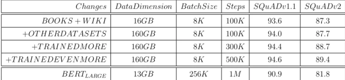
trained with RoBERTa settings for 100 thousand steps with BOOKCORPUS [44] plus WIKIPEDIA English, obtaining a first improvement with respect to the results published in the BERT paper. Then, they performed three more trainings for 100, 300 and 500 thousand steps and combined the last dataset with three more, CC-News [7], OPEN WEB TEXT [11] and STORIES [38], for a total dimension of 160GB. We propose here a summary of the most important results on SQuAD v1.1 and v2 published in the paper [25]:

Changes DataDimension BatchSize Steps SQuADv1.1 SQuADv2 BOOKS + W IKI 16GB 8K 100K 93.6 87.3 +OT HERDAT ASET S 160GB 8K 100K 94.0 87.7 +T RAIN EDM ORE 160GB 8K 300K 94.4 88.7 +T RAIN EDEV EN M ORE 160GB 8K 500K 94.6 89.4

BERTLARGE 13GB 256K 1M 90.9 81.8

Table 3.3: Comparison between RoBERTa and BERT results on QA task using SQuAD Dataset (F1 score)

3.4.2 ALBERT

Differently, ALBERT’s goal is to reduce the dimension of the model and give a speedup in terms of training time. Two main intuitions led to the final “smaller” model: Factorized embedding parametrization and Cross-layer parameters sharing.

(45)

ALBERT promises to be 1.7 times faster than the original BERT and to have 18 times less parameters, which could be seen also as a form of regularization that helps with generalization.

Architectural Choices

As we have said above, BERT uses transformers encoders with GELU which is a non linearity activation function. We will see here ALBERT’s contribution:

• Factorized embedding parametrization: E is the wordPiece (context-independent learning) embedding size, which is directly related to H, the hidden size (hidden layer context-depending learning) and they take normally the same value. It is possible to gain a more efficient use of the total model parameters by separating these two values if H >> E. Since the vocabulary is usually very large and the dimension of the wordPiece[41] embeddings is given by V xE, the increase of H (and E) results in a billion of useless model parameters.

With ALBERT, the authors divide embedding parameters in two ma-trices; in this way, the number of parameters decays consistently from O(V xH) to O(V xE + ExH) when H >> E. They choose to have the same E for all word pieces because these are much more evenly distributed across the documents compared to whole-word embedding [23].

• Cross-layer parameters sharing: This would be also an improve-ment in terms of parameter efficiency. Although there are many ways of sharing, in this work it was decided to use all of the parameters shar-ing across layers. After many experiments, this method led to better results, as shown in tables 4 and 5 in the paper [23].

• Inter sentence coherence loss (SOP): Since NSP was a really triv-ial task and did not have a substanttriv-ial contribution during the training phase, it was replaced by Sentence Order Prediction loss. SOP uses

(46)

30 3. Transformers

consecutive sentences (just like BERT) for the positive samples and swaps its sequence for the negative examples instead of choosing ran-dom sentences from the text.

Model and experimental Setup

In the following table (3.4) all the configuration of ALBERT and BERT are summarized to have a better idea about what changes between the two models, especially in terms of number of parameters:

M odel P arameters Layers Hidden Embedding P arametersSharing

BERTBASE 108M 12 768 768 F alse

BERTLARGE 334M 24 1024 1024 F alse

BERTXLARGE 1270M 24 2048 2048 F alse

ALBERTBASE 12M 12 768 128 T rue

ALBERTLARGE 18M 24 1024 128 T rue

ALBERTXLARGE 60M 24 2048 128 T rue

ALBERTXXLARGE 235M 12 4096 128 T rue

Table 3.4: Comparison between BERT and ALBERT dimensions and number of paramenters

The same dataset used with BERT (BOOK CORPUS + English Wikipedia) was used for the pre-training of the model, by formatting the input in the following way:

“[CLS] sentence1 [SEP] sentence2 [SEP]”.

The system was set to a maximum input length of 512 and a probability of 10% of input shorter than 512. The vocabulary dimension is of 30000 like in BERT but it was tokenized by using SentencePiece[22] like in XLNet[43]. In addition, the masked inputs were generated by using n-gram with n of maximum 3 and for a 125 thousand steps. To conclude the ALBERT chapter,

(47)

we would like to present its results on Question Answering task obtained by using SQuAD v1.1 and v2 in comparison with BERT (Table 3.5):

M odel SQuADv1.1 SQuADv2

BERTBASE 90.4/83.2 80.4/77.6 BERTLARGE 92.2/85.5 85.0/82.2 BERTXLARGE 86.4/78.1 75.5/72.6 ALBERTBASE 89.3/82.3 80.0/77.1 ALBERTLARGE 90.6/83.9 82.3/79.4 ALBERTXLARGE 92.5/86.1 86.1/83.1 ALBERTXXLARGE 94.1/88.3 88.1/85.1

Table 3.5: Comparison between BERT and ALBERT results on QA task using SQuAD Dataset (F1/EM respectively)

3.4.3 DistilBERT

DistilBERT approaches the dimension and the speed problems with an-other technique. The main idea of the study is to create a considering smaller model with the same structure of the bigger one. For example, in DistilBERT the pooler and the token-type embeddings were removed. In addition, it has less numbers of levels. We will explore this model better in sec: 5.3.

For now let us anticipate in a really brief description what they did. They “Transferred” knowledge from the bigger model (BERT) to the smaller one (DistilBERT) by using distillation, considerably reducing the training time as well as the final dimension of DistilBERT.

(48)

(49)

Chapter 4 Question Answering

4.1 Question Answering Problem

Question Answering is that specific field of Natural Language Processing (NLP) which tries to reproduce human behaviour when answering questions posed by humans. In 1960s, the first approaches were called BASEBALL and LUNAR. Both of them had a restricted domain to search answers. After that it was necessary for the research to focus more on improving these techniques in information-retrieval.

One thing which is important to notice is that both of them use a closed-domain. The research is limited to a specific topic, so the questions were given on that context. Recent discovery in NLP (Natural Language Processing) permits to work on opened-domain datasets. In brief, closed-domain datasets and opened-domain ones differ in context, since opened-domain datasets do not have a specific topic. We can divide the question answering problem in four steps, which could be considered as the QA architecture.

The four steps are:

1. Question Analysis

2. Document Retrieval

3. Answer Extraction

(50)

34 4. Question Answering

4. Answer Evaluation

The process flow is shown in the next picture (4.1).

Figure 4.1: Question Answering steps [16]

At the moment, with BERT, it is relatively simple to find an answer to well formulated questions that have a specific right answer. In this task the newest models reached human performances, while understanding if there is an answer in the text, and in case finding it, is still an interesting challenge. A more complex task is to find questions through text comprehension. In other words, it is really difficult to find an answer that needs to capture some text semantics, for example in the case of the answer being distributed in different parts of the text. Anyway, it is possible, thanks to the last research, to consider also open-ended and multi-answer questions.

(51)

4.2 Datasets 35

4.2 Datasets

In all the machine/deep learning applications it is necessary to have a good dataset, from which a model can learn how to solve the problem. The Stanford Question Answering Dataset (SQuAD) [31] was used as a baseline. The SQuAD dataset is the result of crowdworkers work. It consists in questions posed by humans and it is available in two versions, v1.1 [30] and v2 [29]. The second version adds the possibility to have unanswerable questions. This means that some questions do not have an answer in the article under consideration.

The second dataset, the OLP dataset ([6], [5]), is an experimental one. It is still work in progress. The aim of this dataset is to be useful for other text comprehension tasks.

4.2.1 SQuAD v1.1

The first dataset involves more than five hundred articles from Wikipedia and more than a hundred thousand question-answer pairs. In this dataset there is an answer for every question in the paragraph and it is relatively simple for the existing models to reach very good results with this dataset version. This idea was good in order to have a baseline, but at Stanford university it was quickly understood that it would have been better to create a more challenging version. So, less than 2 years later, the second version of SQuAD came out.

4.2.2 SQuAD v2

SQuAD v2 is an extension of the previous version which contains also non-answerable questions. Fifty thousand questions posed to be answerable-like were added by crowdworkers. This means that the dataset is made of 2/3 answerable questions and 1/3 ones. To achieve good results with this dataset, the system should also determine which question cannot find its answer in the text. This version is definitely more complicated than the

(52)

previous one because the system has to analyze the whole paragraph to determine if it is possible to find an answer for a question. For this reason, the models which perform well on SQuAD v1.1 perform significantly worse on this version. Both versions have the same structure, except for the fact that in the second version two keys for each question are added: is impossible and plausible answers. The last one appears only in case of true value on the is impossible (an example of both structure is given in A.1 and A.2).

4.2.3 OLP Dataset

This dataset is, as we have already seen, the result of a workgroup at Bielefeld University. This dataset is composed of a collection of post-game comments from football matches. The difference between the SQuAD dataset and the OLP dataset, except for the structure, is that the first one has a so called open-domain, while the OLP dataset uses a closed-domain instead.

The characteristic of this dataset is that it was thought to consider not only questions with a specific answer in the text, but also situations in which more complex techniques of text comprehension are needed. For example, we can find questions like “How many goals did the player X score?”, so that the answer could be structured in this way; “Player X scored at 33’”, “Player X scored again for the guest team” and so on; the model should use some ontology to understand the relation between the answers and the questions.

Preprocessing and Conversion

Both datasets had completely different structures. For this reason, the fastest way to work with our models and the OLP dataset was to convert it in a SQuAD-like version. A python script was created to extract the text from the csv file. A file for each article by using the information about the number of characters and the sentence number (e.g. B.1), together with the annotation and question (e.g. in B.3 and in B.2) files (they were equally named, so we could easily deal with the association between them) were used to obtain the same structure as in SQuAD at the end.

(53)

4.2 Datasets 37

Since the dataset is still under development at the University, it is not available to the public and we have not released the code yet. With the cooperation of Matteo Del Vecchio and the support of Frank Grimm, we started to study the datasets deeply. Although the datasets were actually completely different in structure, we were able to figure out what the common traits between OLP and SQuAD are.

During this analysis we discovered additional problems and part of the dataset had to be modified. In particular, we worked on problems related to the handmade annotations and fixed some policy which impeded the conver-sion to SQuAD.

In its first version we found different duplications in the annotations files, so we focused our attention on removing all of them and removed redun-dancies in the dataset by using a python script to automatize the process as much as possible. For unexpected cases we had to interfere manually. The second problem derived from the reason why OLP Dataset was born (to have a Question Answering Dataset where the answer had to be the result of some semantic inference, so the answer could not appear directly in the text and could also be composed of different pieces of text collocated far from each other in the article). We often had to deal with this problem, for example we found answer posed in the form “1:0”, to refer to a match result, while in the text the answer was “1-0”, impeding our model to learn by evaluating the answer since they were different. The question file was unique for all of the datasets and, through an id system, we could understand what question an answer referred to. But some of these questions were posed in a general way by omitting a part of the text, for example a name, as we have already shown above. Firstly, we tried to just ignore them but we quickly realized that the dataset dimension became really small. We asked our referent, Frank Grimm, how to deal with this problem and he provided us with a new version with a question file for each article in which all the general questions where specified.

(54)

which is really important for SQuAD, we tried to extract it from the answer file, but there was no assurance about whether the question was answerable or not. For this reason, we suggested to add a tag answerable in the dataset so we could simply set the tag is impossible. In this way, we had just to invert the True or False value in answerable.

The tokenization was not always coherent because spaces were counted directly on the difference between start and end position of tokens, but some-times spaces were treated as token. We had to normalize every situation and find a pattern to automatize this action without losing meaning in the text. Once we solved this aspects, we could convert the dataset and obtain our SQuAD-like version of OLP. The resulting Dataset was split in two parts, the training part and the testing part, to maintain the coherence with SQuAD, but we used also the whole dataset for an evaluation on how good the results were with a model fine-tuned on SQuAD.

4.3 Metrics

The Exact Match (EM) and the F1 score are often used to measure the accuracy in the Question Answering task. The first is basically how many times the output of the model is equal to the ground truth, while the second one considers how “near” the model is when compared to the groud truth. The F1 score is an armonic mean between precision and recall. Let us introduce some definitions to better understand the F1 formula:

• TP: True Positive is when the detection is correct.

• FP: False Positive is when the model says that the prediction is correct but it is not.

• FN: False Negative is when the model gives us a negative prediction instead of the expected positive one.

• TN: True Negative represents all the predictions which are true but in which we are not interested for the current prediction.

(55)

4.4 Before BERT 39

Here we will show the recall and precision formulas based on the notions above: precision = T P T P + F P = T P AllDetection (4.1) recall = T P T P + F N = T P AllGroundT ruth (4.2)

Finally, we can write the F1 formula:

F 1 = 2 ∗ precision ∗ recall

precision + recall (4.3)

4.4 Before BERT

Before Transformers were invented there was some approach to the Ques-tion Answering problem. Here we give an example of some older models, precursors of the more recent BERT.

4.4.1 BiDAF

BiDAF (Bi-Directional Attention Flow) [34] is a closed-domain QA model which can only answer questions with a string in the text. It was the State of Art before ELMO and BERT. This model is composed of 3 main parts: the Embedding layers, the Attention and modeling layers and the output layer.

The Embedding layers are three different levels of embeddings: character, word and phrases embedding. As we have already said, this part transforms words information into their real-valued vectors representation.

The Attention and model layers add context about the query by using additional information and merge everything in a unique output, which is called “Query-aware Context representation” in the paper.

The last layer transforms all the information received from previous layers into probabilities values, which will be used to calculate the start and end positions of an answer.

(56)

Figure 4.2: BiDAF

4.4.2 ELMo

Not only does the idea of ELMo (Embeddings from Language Models) [28] take into consideration the following word that can appear in a sentence given the current word, but also the previous one, obtaining different embeddings for the same word. It is the first time this kind of contextual approach has been used, while before a fixed embedding was assigned to each word. To do that ELMo needs to be trained on a huge dataset and it uses a bi-direction LSTM (sec ??). The first direction is forward and considers information about the following word, while the second network goes backward to consider the previous word.

ELMo was used for Question Answering on SQuAD v1.1 by adding it to an improved version of BiDAF. This led to an improvement of 4.7 percents compared to the baseline, as shown in the relative paper.

(57)

4.5 Results Comparison 41

Figure 4.3: ELMo

4.5 Results Comparison

In the next table 4.1 a little recap. We will give an overview of all the most significant results published in the papers of each model:

M odel SQuADv1.1 SQuADv2 BiDAF 68.0/77.3 −/−

ELM o −/85.8 −/− BERTLARGE(single) 84.1/90.9 78.7/81.9

RoBERT a 88.9/94.6 86.5/89.4 ALBERTXXLARGE 88.3/94.1 85.1/88.1

Table 4.1: The most significant results in Question Answering, given with EM/F1 metrics

(58)

(59)

Chapter 5 DistilBERT

5.1 Models Compression

From the literature we learn that there are many techniques to reduce a model dimension and compress it to a smaller form losing something in precision but gaining in lightness and speed. We are more interested in Knowledge Distillation since it is the technique used to train DistilBERT5.3. We are going to explain it more in details in the next section 5.2.

5.1.1 Pruning

This is a technique to prune weights that match a certain criterion by as-signing the value zero to them. The most common pruning criterion consists in comparing an absolute value to a threshold. If that value is smaller than this threshold, it is set to zero, because a low value contribute only a little for the final results and can be directly removed. This method was born to contrast the over-parametrizetion of models and redundancy in logic and features. There are two ways to do pruning: one-shot pruning and iterative pruning. The first one is done only once, while the second one of course more than once, but changing the pruning criterion every time (iteration)1_.

1_{https://nervanasystems.github.io/distiller/pruning.html#pruning}

(60)

44 5. DistilBERT

5.1.2 Quantization

Quantization reduces the precision of the values from the most widespread FP32 (32-bit floating point) to a half precision FP16, or even to a lower representation like 8-bit integer, but preserving the same accuracy. This also leads to a reduction in terms of storage, estimated to be 8 times smaller by using 8-bit integer instead of 32-bit floating point2_.

5.1.3 Regularization

“Any modification we make to a learning algorithm that is intended to reduce its generalization error, but not its training error.”[13]. We are not really interested in this method, so we refer to the link at the bottom of the page3 _{for a deeper study.}

5.2 Knowledge Distillation

Knowledge Distillation (KB) could be seen as a transfer learning technique, even though it has a different aim. In this case we want to obtain a smaller network from the pre-trained one by transferring not its exact weights but its way to generalize the task. It is more correct to say that Knowledge Distillation’s goal is something more than barely transferring knowledge, but it is also a form of compression from a huge high precision model to a smaller one, without losing too much in generalization.

It is a reinforcement learning technique which wants to reduce the di-mension of huge models (like BERT) and the training time by transferring knowledge between two models. In particular, Teacher-Student paradigm is composed of a small network, the Student, and a bigger one, the Teacher, which should be trained on the complete dataset.

The training phase usually needs a consideably amount of time for models

2

https://nervanasystems.github.io/distiller/quantization.html

(61)

5.2 Knowledge Distillation 45

like BERT and also its dimension and response time do not help to execute and use them in edge devices. The final aim is to teach the Student how to simulate the Teacher’s behaviour. Let us define the two behaviour as ϕT and ϕS _.

In the case of the transformer distillation MHA (Multi-Head Attention) and the FFN (Feed-Forward Network), the output could be used as behaviour functions. The Knowledge Distillation can be modeled by minimizing the following function:

LKD =

X

x∈χ

L(ϕs(x), ϕt(x)) (5.1)

where χ is the dataset, x the next text input and L(.) is the loss function destinated to evaluate the differences between the student and the teacher predictions. We will introduce, explaining more in details the distillation, notions like Student-Teacher network 5.2.1, softmax with Temperature 5.2.2 and Dark Knowledge 5.2.3.

5.2.1 Teacher-Student

As it was already anticipated the Teacher is the bigger high precision network used to transmit the “behaviour” to the Student network. Firstly, the Teacher network has to be trained over the complete dataset with high performances. Secondly, when a Student is built, there has to be correspon-dence between intermediate levels since they are different in dimension. The pipeline is quite simple and it can be summarized in this way: the same input passes through both models, the Teacher and the Student, producing their output that is fed to the softmax. This is a key point because here we find a special version of softmax, the softmax-temperature (5.2.2), which produces soft-labels from the output of the Teacher and soft-predictions from the Stu-dents output. Then the Loss function is calculated between them. The same Temperature is used and this part is the Distillation Loss. Also the hard prediction of the Student model is calculated by using the normal softmax, which will be compared to the Ground Truth obtaining the Student Loss.

(62)

46 5. DistilBERT

Finally, both results are summed together to obtain the final Loss:

L(x; W ) = α ∗ H(y, σ(zs; T = 1)) + β ∗ H(σ(zt; T = τ ), σ(zs, T = τ )) (5.2)

Where x is the input of the model, W are the student’s weights, σ is the softmax (also with the Temperature T ), y are the labels of the Ground Truth and H is the Cross-Entropy loss, while z represents both Student and Teacher logits. The following picture (5.1) shows graphically the formula 5.2 above:

Figure 5.1: Teacher-Student Model schema [20]

5.2.2 Softmax-Temperature

Softmax-temperature is a standard Softmax with a coefficient that makes the predictions of a network “softer”. In fact, if we compare the two formulas we can easily notice that the only difference is in this T , which divides the network logits. pi = exp(zi) P jexp(zj) (5.3) pi = exp(zi T) P jexp( zj T) (5.4)

(63)

5.3 DistilBERT Model 47

Where the 5.3 is the standard one and the 5.4 is the Softmax with tempera-ture.

This is the baseline of the Dark Knowledge in explained in the next section (5.2.3).

5.2.3 Dark Knowledge

Dark Knowledge is the result obtained from the application of Softmax-Temperature to the Teacher network prediction, adding more information to the class that the Teacher found to be more probable. This additional knowledge is the so-called Dark Knowledge [21] that we want to transfer from the Teacher network to the Student. As we have already said in the previous section 5.2.1, the soft-prediction of the Student is done by using the same value of Temperature.

5.3 DistilBERT Model

Since BERT is a mastodontic model and requires a lot of time to train and a significantly computational effort, the HuggingFace research group [12] model tried to combine the Knwoledge Distillation with BERT. In addition, the token-type embeddings and the pooler were removed, because they re-alized that the next sentence classification was not so effective. The rest of the architecture was kept identical but the number of layers was reduced of a factor of two. As a result, a smaller language model, DistilBERT, was born. This was trained with BERT supervision compressing it and preserving almost the same performance as BERT.

To transfer the knowledge in DistilBERT, this was trained on the soft target probability of the Teacher:

LCE =

X

i

ti∗ log(si) (5.5)

ti and siare calculated by using a softmax-temperature 5.4, where T is always

(64)

48 5. DistilBERT

was set to the same value, both for Teacher and the Student at training time, while at inference time it is set to 1 (the standard softmax), to calculate the hard prediction of the student. The code below shows how the knowledge was distilled during the fine tuning phase of DistilBERT. The formula is calculated in the run squad w distillation.py4_:

Listing 5.1: Loss with distillation used during Fine-Tuning

l o s s _ f c t = nn.K L D i v L o s s( r e d u c t i o n =" b a t c h m e a n ") l o s s _ s t a r t = l o s s _ f c t( F.l o g _ s o f t m a x( s t a r t _ l o g i t s _ s t u / a r g s.t e m p e r a t u r e, dim = -1) , F.s o f t m a x( s t a r t _ l o g i t s _ t e a / a r g s.t e m p e r a t u r e, dim = -1) , ) * (a r g s.t e m p e r a t u r e ** 2) l o s s _ e n d = l o s s _ f c t( F.l o g _ s o f t m a x( e n d _ l o g i t s _ s t u / a r g s.t e m p e r a t u r e, dim = -1) , F.s o f t m a x( e n d _ l o g i t s _ t e a / a r g s.t e m p e r a t u r e, dim = -1) , ) * (a r g s.t e m p e r a t u r e ** 2) l o s s _ c e = ( l o s s _ s t a r t + l o s s _ e n d ) / 2.0 l o s s = a r g s. a l p h a _ c e * l o s s _ c e + a r g s. a l p h a _ s q u a d * l o s s

while the following code comes from the file distiller.py in the same reposi-tory:

Listing 5.2: Loss with distillation used during Training

l o s s _ c e = (

s e l f. c e _ l o s s _ f c t (

F.l o g _ s o f t m a x( s _ l o g i t s _ s l c t / s e l f.t e m p e r a t u r e, dim = -1) ,

(65)

5.3 DistilBERT Model 49 F.s o f t m a x( t _ l o g i t s _ s l c t / s e l f.t e m p e r a t u r e, dim = -1) , ) * (s e l f.t e m p e r a t u r e) ** 2 ) l o s s = s e l f. a l p h a _ c e * l o s s _ c e

According to the results published on the DistilBERT paper [33], it can reach 97% of BERT understanding skills, despite being 40% smaller and 60% faster. For completeness, these results are summed up in the table 5.1 with the GLUE baseline [33].

M odel Score CoLA M N LI M RCP QN LI QQP RT E SST − 2 ST S − B W N LI ELM o 68.7 44.1 68.6 76.6 71.1 86.2 53.4 91.5 70.4 56.3 BERT − base 77.6 48.9 84.3 88.6 89.3 89.5 71.3 91.7 91.2 43.7 DistilBERT 76.8 49.1 81.8 90.2 90.2 89.2 62.9 92.7 90.7 44.4

Table 5.1: Comparison of DistilBERT’s results with BERT-base’s and ELMo performance

DistilBERT can preserve most of the results of BERT-base on SQuAD v1.1 or about 2 point less and even better, adding an ulterior step of distil-lation during the fine-tuning phase. The results are shown in the next table (5.2), where the double distillation process is indicated by a (D). Both mod-els are incomparable in terms of lightness, since DistilBERT has 66 million of parameters against the 110 of BERTBASE. It gets good results also on

in-ference time because BERT-base needs about 668 seconds, while DistilBERT 410 seconds 5.2.

M odel IM Db SQuAD(EM/F 1) BERT − base 93.46 81.2/88.5

DistilBERT 92.82 77.7/85.8

DistilBERT (D) − 79.1/86.9

(66)

50 5. DistilBERT

M odel P arameters(millions) Inf erence(seconds)

ELM o 180 895

BERT − base 110 668

DistilBERT 66 410

Table 5.3: DistilBERT number of parameters and speed

One further advantage of having less dimension and inference time is that we can execute the model on edge devices (that could be a smartphone), which do not have enough memory and computational power to execute the whole BERT in an acceptable amount of time. The HuggingFace team also managed to build an android application with the tensorflow version of DistilBERT for question answering5.

(67)

Chapter 6 QADistilBERT

6.1 QABERT

This version of Question Answering level was born from the collaboration with Matteo Del Vecchio during the “projekt” at Bielefeld University, which had the aim to start getting our hands on the existing NLP models.

QABERT is a task specific implementation of question answering level for BERT. We thought about what could be the benefit of developing a different architecture of this layer. For this reason, we implemented 5 combinations of fully connected layers and activation functions, in total, three models with 2 fully connected layers, each of them with an activation function among ReLU, GELU and Tanh, and two models with 4 fully connected layers with GELU or ReLU between couple of layers. In the following sections we will show come images we have created to have a graphical look at their compositions.

6.1.1 QABERT Vanilla

This was only to have a BERT-like baseline, since we did not have access to the same hardware of google. We fine-tuned the vanilla version just like the BERT QA level was developed by google. It does not use any activation function and has an input shape (batch size, max seq length, hidden size) and output (batch size, max seq length, 2 ).

(68)

52 6. QADistilBERT

Figure 6.1: QABERTVanilla model schema

6.1.2 QABERT 2L

To explore the benefit of having more layers, we added two layers on the top of BERT and tried different activation functions to understand which one works better. We did this in order to achieve better results on question answering. We also tried different configuration shapes and we will present only the best ones. The idea was to have a conic function reduction of the dimension; in this way we could have a more gradual reduction from the BERT output dimension to 2.

QABERT 2L Tanh

In the version with Tanh function we opted for a reduction, firstly, from 768 to 384, and then from 384 to 2 (Figure 6.2).

(69)

6.1 QABERT 53

QABERT 2L GELU

The second version of this model uses the GELU (Gaussian Error Linear Units) activation function, which is used in BERT [14]. The conic in this case decreases from 768 to 256 and from 256 to 2 (Figure 6.3).

Figure 6.3: QABERT2LGELU model schema

QABERT 2L ReLU

With ReLU activation function the same input dimension was kept in both layers since the skip idea was introduced. The output of BERT is fed to the first layer and then added to its output before feeding everityng to the second layer (Figure 6.4).

(70)

54 6. QADistilBERT

6.1.3 QABERT 4L

With four layers we were able to develop a different idea of shapes reduc-tion. In this case we had more layers and we thought about a more “rhombic” idea. In fact, the shape increases its dimensions between the first two layers and uses the same conic concept as above for the last layers.

QABERT 4 ReLU

This model uses the ReLU activation function between the layers and the shape, as we have already said, which are firstly enlarged from 768 to 1024 and reduced from 1024 to 200 and from 200 to 2 at the end (Figure 6.5).

Figure 6.5: QABERT4LReLU model schema

QABERT 4 GELU

We will introduce another idea which consists in using to use only the “rhombic” dimensions changing. The skip idea wants to take more into account the BERT output. The third layer input thus has a dimension equal to BERT output. As it is shown in the next picture, the original BERT output is added to the second fully connected layer’s output. We will use this question answering level as a baseline for our study because, looking at the results we obtained by fine-tuning BERT with different configurations, this structure reached better results with respect to the others (Figure 6.6).