Scuola di Ingegneria dell’Informazione
Master of Science in Automation Engineering
A Modelica library For Mixed-Phasor- and Time-domain
Simulation Of Electric Networks
Supervisor: Prof. Alberto LEVA
Master Thesis by: Ahmadreza ARFAEI Matr: 764493
Acknowledgements
First of all I would like to express my utmost gratitude to my supervisor Professor Alberto Leva for his guidance, encouragement and useful Hints. His valuable ad-vices and consistent availability are indispensable.
I owe my deepest gratitude to all my professors Specially Professor Frannco Zappa and Professor Ricardo Scattolini.
Thanks to my father Hossein, who has always been a role model for me in my life, to my mother Zarrintaj who has supported me in everything.
Finally, special thanks to my MohammadAli Aghakhani,Ali javadizadeh and ShahabReza Besharat and many others who walked with me all the way along for consistent cheering and supporting.
Chapter 1
Introduction
This chapter briefly introduces the context of the presented work and states the main problem addressed, and sketches out the organization of the document.
1.1 Overview
Electricity production continues to grow around the world and Global electricity production increases by 2.4 percent per year over the projection period, from 16,424 billion kilowatt-hours in 2004 to 30,364 billion kilowatt-hours in 2030. In such a scenario , The business energy market is in desperate need of reform.
Growth trend of the market is main reason for which modeling and simulation are become matter of research interest nowadays. On the other hand integrating such new methods via some novel and revolutionary technological advances bringing up the efficiency and decrease computational efforts.
The past few years have seen countless research topics on utilizing renewable energy sources (such as solar thermal and photo-voltaic sources) due to depletion of fossil fuels and their high environmental impacts. Thus each plant turns out to be a power producer. The main problems with these energy sources are cost and availability.
Smart grids promise to facilitate the integration of renewable energy and will provide other benefits as well. This technologies can help provide real-time readings of the power line, enabling utilities to maximize flow through those lines and help alleviate congestion. As smart grid technologies become more widespread, the electrical grid will be made more efficient, helping reduce issues of congestion. Sensors and controls will help intelligently reroute power to other lines when necessary, accommodating energy from renewable sources, so that power can be transported greater distances, exactly where it's needed.
In favor of the smart grid technology, the energy production is distributed among many producers rather than massive plants. In some regions, individuals can contribute to energy production on the distribution grid by generating electricity at their home for example, solar on rooftops. Where available, enhanced net-metering incents consumers to sell power back to the grid during peak pricing hours. so consumers make money and utilities are able to better manage peak demand. Whole neighborhoods could become solar or wind generation plants, introducing excess power back into the grid to meet demand.
Of course there is much more to the idea of smart grid than the matter just explained, but accepting this fact is enough to realize what is relevant in the context of this dissertation.
Distributed generation(DG) , as a new form of clean energy generation , provides flexible power supply support for electric power system. But DG capacity generally is smaller, lower voltage levels, and it is incorporated into electric power system at distribution network side. Therefore, DG incorporated into electric power system has brought many unprecedented problems, DG has a negative effect on power system stability, power system control and protection.
Of course, a distributed network can be modelled and simulated, to examine the couplings among its smart grids, and the effects of the attachments
and detachments of smart grids with respect to the network. Based on the outcome of the simulations, the attachments and detachments of smart grids can then be scheduled properly if this is possible, and convenient control solutions can be devised and assessed in the opposite case, in order to prevent -or at least mitigate- hazardous failures. Hence, the task of simulating the effects of smart grids on the network holds a particularly relevant importance.
1.2
Background And Motivation
Simulation of AC network split into three operating points : Rapid transient ,quasi-stationary and steady-state. Analysis of AC network could be carried out by in either time domain and phasor domain .consequence of adoption of phasor-based approach is highly efficient simulation with less computational effort.
In the first case, rapid transient, there is completely different story and obviously the frequency is not a constant term. Therefore dynamic models are considered and network has to be analyzed in time domain.
In second case, quasi stationary, phasor approach can be extended by means of so called “swing equation” which turn algebraic phasor framework to a dynamic one, introducing machine angle as the state variable.
AC quantities , such as currents and voltages, are expressed with an amplitude and phasor . Meanwhile in steady-state point it is obvious that the network frequency is constant. Thus we can shift into the phasor representation.
Let’s consider the network in stationary mode .All signals expressed in phasor domain. As a consequence computation power and memory allocation reduced which brings up computational efficiency. If the frequency is influenced by some abrupt event , like opening or closing switches , phasor model cannot be
utilized and then time domain representation adopted which describe voltages and current in more details. The main idea behind the mixed approach is to utilize impedance relations when the frequency is constant as in the case of phasor type simulators, and to utilize differential equations in time domain when the system is transposed to non-sinusoidal signals as in the case of transient type simulators.
Usually phasor type Modelling is preferred over the transient type due to the its better computational efficiency when the simulation size is great. The phasor type simulators are constructed based on the assumption of constant frequency and consequently neglect the transients [4]. As mentioned, the phasor type simulators are preferable when the magnitudes and the phases of voltages and currents at the line frequency are of the interest.
Focusing on two mention cases above , it become highly profitable and favorable that merge two models and write both equations to a single component which could switch back and forth between two phasor and time description possibly in automatic manner.
the main issue is how to join two modelling approach in a library of object-oriented ( that is context-independent) models of some mostly used components in electrical systems. Managing the switch between two domain is a bit tricky in object-orienting modeling and simulation approach. events triggering actions which lead to transition from time to phasor and vise-versa are mostly local.
1.3
Outline of the Thesis
This disertation is organized as follows. Chapter 2 addresses a Modelica library which is formed by set of components .This modelica library targeted to the purpose of this work, to be consecutively prolonged from a proof of concept
to a production tool. Chapter 3 provide more simulation examples of proposed approach to report the obtained advantages and to illustrate the viability of the proposed approach. Chapter 4 ends this thesis with some conclusion and sketches out future work.
APPROACH???????
2.1
FOREWORD
The increasing availability of high performance relatively low cost computers in recent years has presented exciting new opportunities for power utilities to use
advanced computer based modelling, system analysis and optimization strategies for the management of systems.
These have ranged from expert system methodologies, neural networks to the application of object oriented methods to power networks covering switching operations, protection, restoration, fault-diagnosis and the integration of advanced Energy Management Systems (EMS)
The growing number of customers and the various supporting technologies has resulted in large and extremely complex networks. In the past, system administrators and planners had an overview of the technological criteria for the design, expansion and maintenance of the network. However, it is now much more difficult to manage these tasks because of the greater network complexity and the increasing amount of data to be processed.
As electricity supply is a dynamic sector, it is essential that the network model under development be representative and easy to maintain and extend. It was decided to use object-oriented techniques for the development of a unified network model; the resulting model being implemented in a database system.
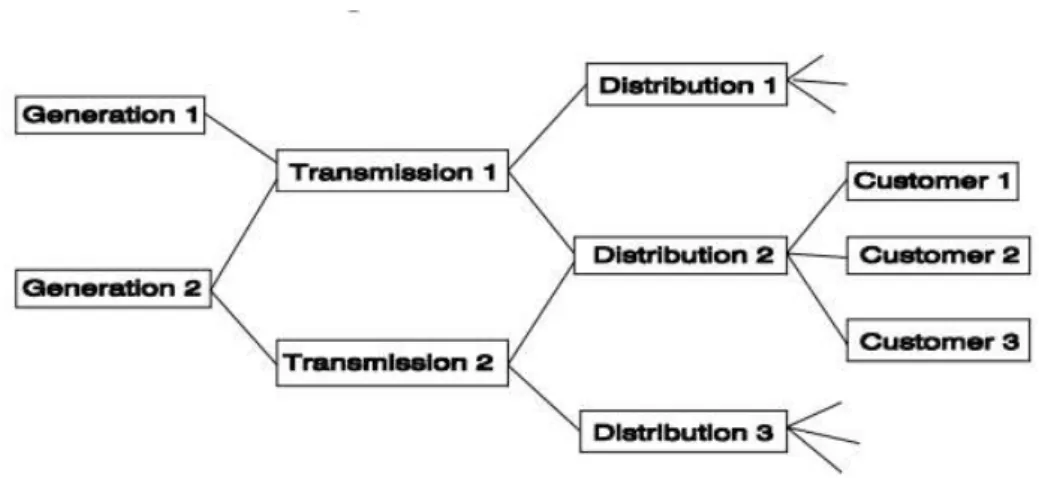
The basic structure of an electrical power system can be considered to consist essentially of a set of nodes and links. The node could be a component of a power system, such as a generator, transformer, switchgear etc. A link is a conductor which connects nodes together. Therefore, an overhead transmission line and underground cables etc. could be elements within a link. A specific example of an electrical power network is shown in Figure 2.1
Figure 2.1: Power network is shown as nodes and links
In any real case, an electric distribution network comprises a high number of smart grids. For the sake of scheduling the detachments/connections of smart grids to the network, observing their coupling with each other and their combined effect on the whole network, the network needs to be simulated as a whole entity.
In addition, the reliability analysis of the power grids is difficult since they are made up from thousands of components. Even though the failure modes of the each component may be known, in a power grid these values can differ since they are not independent from each other.
2.1. OBJECT-ORIENTED MODELLING
This section introduces the basic principles of object-oriented modelling . In an object-oriented model, the object and their associations correspond directly to real world entities and their relationships. As a result, the object model is highly modular and closely resembles the real network.
These characteristics make the model easy to understand, maintain and extend. A major difference between object-oriented modelling and other
approaches is the inclusion of the dynamics of a system in the objects. Objects are therefore self-contained structures and the resulting system is highly modular.
Modularity significantly enhances the maintainability and extendibility of the system. Further on-going development of the object model is possible, even after it has been installed, because the object schema can be continuously evolved.
2.1.1. MODELICA LANGUAGE
Because of the open architecture of Modelica which allows to modify the existing components, thus there is the possibility of employing impedance relations although Modelica is design for PDEs originally, the proposed mixed approach can be implemented in Modelica.
The importance of the openness of the simulation tool to possible modifications increases as models and control methods on the electric network are being evolved regularly, thus a general model is out of topic. Together with its open source nature, Modelica and the other simulation tools developed on it respond to the demands and expectations from a simulation tool stated in [2]. The advantages of Modelica over many other simulation languages at dealing with components from many engineering domains [3] gives the possibility of extending the electrical domain modeling to multi domain modeling with internal control algorithms when needed.
Another advantage of Modelica is the object oriented principle and the casual modeling. While object-oriented concepts enable proper structuring of models, the capability of non-causal modeling makes it easy to model for example power lines which are quite cumbersome to model using block-oriented languages such as Simulink [18]. As a consequence, from the viewpoint of this
work, Modelica solves the systems in object oriented fashion, if one can achieve modeling the impedance relations in the same style as in the section 3.2, it is even possible to model the networks with the most cumbersome and complex mathematical expressions. That is to say for the author's convenience, Modelica is preferable over the modeling and simulation tools that use block diagrams when dealing with complex topologies.
In synthesis, the suggested mixed approach which has phasor models and time-domain ones co-exist, using the former type when frequency is constant and switching back/forth to the other when this is not (temporarily) true owing to some abrupt event, is not implemented in the conventional simulation environments.
2.2. STRUCTURE OF THE LIBRARY
The library compromise of the most primitive models, like resistors, capacitors, inductors, grounds and power sources and etc. Thus validating the approach in the component level and then increases complexity step by step until the level of complex topologies like the whole electrical network is achieved.
Chapter 2
Introducing The Modelica Library
This chapter starts with a description of the library structure as resulting from the proposed approach . Then follows by illustrating some examples the idea of co-existing time and phasor domain at component level.
As anticipated, phasor models in Modelica are not a novelty [1, 2], and as such, the proposals that we are making with this paper are to be integrated in the scenario depicted by works like the ones just quoted.
However, this study has some specific peculiarities, a discussion on which (and the consequently proposed solution) provide the main contributions of this work. Specifically, three aspects are herein addressed:
creating models that contain both a phasor and a time domain description of a given component.
managing the transition (changeover) between the two at the component level.
managing the decision to make a changeover at the overall model level.
For simplicity, at this point, the transitions between domains are depended on the system level, thus the user controls the switching rather than an event enforces it.
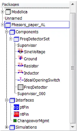
Figure 2.0: Illustration of the the developed library
We now consider the problem of mixing phasor and time domain descriptions in the same component model, and of managing at that level the changeover between the two.First, physical connectors are needed to be defined. To this end, a positive/negative phasor and time domain pin is straightforwardly defined.
2.0. The Approach
The need for modelling in the context of (AC) electric networks and their management has been recognized since long time ago. The introduction of renewable energies and distributed generation has then increased the interest on the matter in the last decades, and further impulse to the mentioned research has been coming from smart grids. Nowadays, simulation models of electric networks are also often combined with those of the generator’s prime movers to form multi-physics, multi-scale and potentially large overall models, for which the object-oriented paradigm of Modelica is particularly suited.
In such cases, however, the electric part of the model is often the bottleneck for simulation efficiency, and the reason for that is structural. In extreme synthesis, in fact, an AC network can be modelled at three levels. The most efficient one from the computational standpoint is provided by phasors : this framework allows to write an algebraic model, that however is valid only in the hypothesis of a single, constant frequency for all the network. Small fluctuations of “local” frequencies are allowed by the so-called “swing equation” formalism, Quite intuitively, the idea of using phasor models in Modelica is not new, but to the best of the authors’ knowledge, to date no attempt was made to have phasor and time domain descriptions co-exist at the component level. For example, in [1] the idea of coupling phasor-domain and “transient” models is introduced, but the connection between the two relies on causal signals, making it difficult to represent it at the individual component level, especially for what concerns the domain changeover. Another interesting paper is [2], where however no changeover to time domain is considered, and the possibilities of phasor-based modelling are exploited via a convenient use of the swing equation. As such, even a minimal literature analysis like that reported indicates that the problem
addressed herein is of both theoretical and practical interest, and that the attempted solution has some novelty characteristics.
2.0.1 System-level modelling
We now move to the problem of managing the changeover between the time domain and the phasor representation at the level of the entire simulation model, i.e., of the network—in synthesis, thus, we specify how the Timedom flag is handled. Switching from phasor to time domain is generally the consequence of some abrupt event known to at least one component, like for example a closing or opening switch. It is thus assumed that in such a case, the affected component directly sets the flag to true, causing the changeover instantaneously.
A bit more difficult is conversely the reverse changeover, since to make it feasible, all the currents and voltages need settling to a sinusoidal regime. The decision is in this case taken on the basis of local signaling from the components, and of a unanimity verification mechanism at the system level.
2.0.2 Local signalling of sinusoidal regime
Also in this case, like it was for the component-level changeover management shown in Section 3.1, the main goal of model design is to avoid unnecessary events, for efficiency reasons.
Suppose therefore that we need to detect if a certain variable x(t) – voltage or current – is “sufficiently” close to a sinusoid with frequency freqHz, assumed for the moment of zero mean for simplicity (releasing this is straightforward, see later on). Filtering x(t) through the continuous-time transfer function
F(S) := 𝑋𝑓𝑋(𝑠)(𝑠)
=
(
1
𝜋𝑓̥
𝑠
1+
𝜋𝑓̥ 𝑠+
𝑠2 (2𝜋𝑓̥ )2)
(2.0)produces an output xF(t) equal to the input x(t) if and only if the frequency of the latter is exactly 𝑓 , which is apparently set to freqHz.
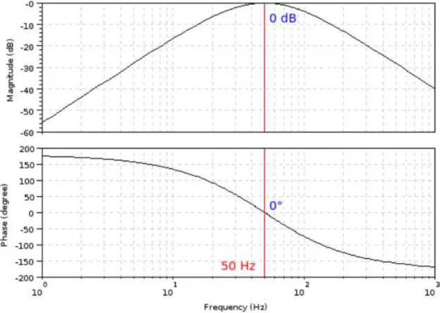
Figure 2.1: frequency detector – Bode plots of F ( jw )
Parameter nF is used to enhance the attenuation of the frequency response F (jw) as the input frequency moves away from fo, and a value of two (or three at most) proved enough in practice. The operation of F(s) is shown by the Bode plots of Figure 2.1, obtained with fo = 50 Hz and nF = 2.
The output of F(s) in (2.0) is then used, together with its input, to form the signal
s(t) =
1+𝑥𝑓̥(𝑡)2
1+𝑥(𝑡)2
(2.1) which is structured so as to inherently avoid division by zero errors, and finally s(t) is lowpass-filtered by the unity-gain first-order block
D(s):=𝑌(𝑠) 𝑆(𝑠) =
1
1+𝑠2𝜋𝑓̥ 𝑘𝑓̥ (2.2)
where parameter kf is used to control the achieved smoothing (a value of ten is a good default). As a result, y(t ) will signal the required condition on x(t) by taking a value very close to the unity, with small fluctuations.
Comparing the value and the time derivative of y2(t) to suitable thresholds, where squaring the signal is to avoid the events that would be generated if its absolute value were conversely taken, is therefore a means to detect that x(t ) is close enough to a sine wave with frequency freqHz.
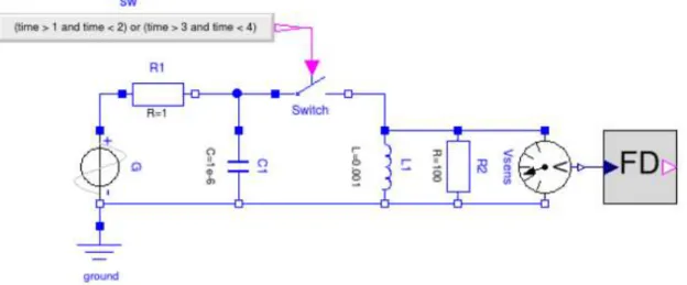
Figure 2.2: frequency detector test – Modelica diagram
To show the efficacy of the proposed technique, and also its autonomy with respect to the rest of the proposed modelling paradigm, Equations (2.0) through (2.2), together with the mentioned thresholding mechanism, were turned into a FreqDetector block, that is used in the model of Figure (2.2) together with
components from the Modelica.Electrical library (its use in the presented one, with the actual introduction of phasor modelling, will be illustrated later on).
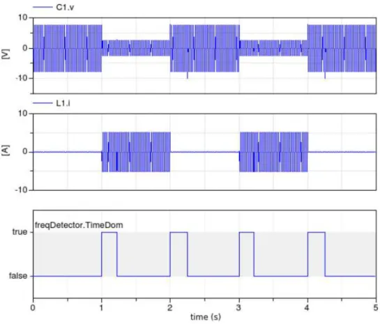
Figure 2.3: frequency detector test – simulation results
Figure 2.3 shows a sample simulation test. Detailed figures are inessential for its purpose, apparently, but as can be seen, the need for time domain modelling as caused by the switch closing and opening is detected correctly, especially for the transition toward (the possible use of) phasor mode. Recall that the symmetric transition is in any case guaranteed by the locally originated signaling.
This is because the phasor to time domain transition must be instantaneous to preserve accuracy, while if the time to phasor domain on is delayed with respect to the time when it is acceptable, the only relevant effect is some waste of CPU time. It is worth noticing that the 5s simulation of Figure 2.3 involves only 14 state events, which would apparently not be true if the possibility of switching to phasor mode were identified based on zero crossing counters, or similar
methods. Note also that the proposed technique introduces some additional state variables, but these pertain to linear, time invariant, causal blocks cascaded to the physical model. The resulting simulation overhead is thus modest, and in any case much lower than that of zero-crossing or similar methods.
The default values chosen allow for a safe transition toward phasor modelling, without bounces and within a reasonable time. In the presence of an essentially constant-frequency behavior interspersed with abrupt events that make the frequency content of the involved signals radically different from the (quasi-stationary) one, this is a good compromise between fast transition to phasor mode (which undoubtedly favor’s simulation efficiency) and possibly undue switching of the two modes (which conversely may be detrimental owing to re-initializations). Also, the presented detection method is inherently normalized, since so are all the involved quantities (except times, of course).
This makes the selected default values for the involved parameters valid in a wide operating range, and for an equally wide variety of network physical parameters. To manage a possible nonzero average of u(t ), finally, the proposed filtering path is implemented as a series of transfer function blocks from the Modelica Standard Library, and signal s(t) in 2.1 is formed by taking the output of the first block in the place of u(t). This ensures that the average of the signal taken as input settles to zero with a dynamics comparable to that of the transients superimposed to its steady-state sinusoidal behavior, and at the same time preserves the exploitation of the unity-magnitude and zero-phase frequency response values at the sought frequency so as to realize the envisaged detection system.
2.0.3 System-level handling of TimeDom
To manage the TimeDom flag at simulation time, denote respectively with Npt and Ntp the number of elements entitled to cause a changeover toward time domain mode (typically, switches), and that of elements the voltage across which is to be checked to approve the reverse transition.
From a conceptual standpoint this set could well be the totality of the present passive components, but for optimization reasons the user can be allowed to introduce “frequency probes”, based on the described FreqDetector component, only where deemed necessary.
At the present state of the library development, this architectural choice is still open: most likely, however, based on the experience that is being gathered, the final solution will be to distinguish a “basic” mode, where any passive component has a detector, and an “expert” one, where the user is free to configure the mechanism at his/her best convenience.
In any case, assuming – in principle, as the implementation described in the following section is different for efficiency reasons – two Boolean vectors P2T and T2P, of length Npt and Ntp respectively, to be declared at the outermost model level, and omitting trivial details on the inner/outer manner they are managed, the following procedure for handling TimeDom is adopted.
1. The simulation starts out in time domain mode,for the safe side (possibly, in the future, unless differently specified in the “expert” mode). All the elements of P2T and T2P are conveniently initialized (at present, to false).
2. All entitled elements manage their local time domain flag based on the contained FreqDetector element, and the system-level T2P vector collects them all.
3. If at the system level time domain mode is in use,and all the elements of T2P are true, then the system switches to phasor domain mode.
4. If at the system level phasor mode is in use, any transition to true of at least one element of P2T causes a changeover to time domain mode, with the required re-initializations.
2.0.3 Modelica implementation
The solution just described serves the intended purpose, and the realised one is totally equivalent from a conceptual and functional standpoint.
However, if said solution were implemented literally, some deviation from a totally object-oriented setting would be involved, since any component participating in either of the two mentioned Boolean vectors, would have to contain suitable parameters to indicate which position in said vectors pertain to it. The responsibility of setting those indices correctly would stand with the user, being possibly complex and cumbersome to manage for large models.
In addition, and most important, even if the management of the mentioned indices were somehow automated, some model connections would in this way be realised, that do not fall under a proper connector abstraction.
To overcome this relevant problem, the described solution is therefore implemented as follows. First, a ChangeoverMgmt connector is defined as shown below
connector ChangeoverMgmt
flow IntegerNtp "# o f T >P voters" ; flow Real ForceP2T ;
flow Real AllowT2P ;
Modelica.SIunits.Frequency freqHz ; Boolean TimeDom ;
Real dum " Squelch balancing warnings " ; end ChangeoverMgmt ;
Listing 2.0 : the ChangeoverMgmt connector
Each component participating in the changeover decision (i.e., each model of reactive elements or of commuting ones like switches), and also each generator, is endowed with such a connector, named in the following C; also, all those models take the TimeDom flag and the (nominal) frequency from that connector.
Reactive components (the Inductor model is an example) furthermore contain the code :
C.Ntp = 1 ;
C.Fo r ceP2 T = 0 ; . . .
C.AllowT2P =if C.TimeDom and not FD.TimeDom
then -1 else 0 ;
The first line reported in Listing 2.1 provides the Supervisor component, described later on and that also has a ChangeoverMgmt connector to which those of all network elements are connected, with the number of those elements that vote for the time domain to phasor mode transition.
The second line means that the component, given its role, is not entitled to force a transition from phasor to time domain model. The last reported line, finally, casts the vote when this is required.
Models of commuting components (like switches) conversely contain the code
parameter Real Tsw = 0 . 0 1 ; parameter Real thrsw = 0 . 0 1 ; . . . Real xsw ( start = 1 ) ; . . . xsw +Tsw * der ( xsw ) = if control then 1 else 0 ; C.ForceP2T = if control and xsw <1 thrsw or not control and xsw> thrsw then 1 else 0 ;
Listing 2.2 : model of switches
When the Control input (the switch command) commutes, the introduced dynamic variable xsw is used to generate a square pulse with a minimum of state events, and this is in turn used – see the last line in Listing 2.2 – to signal that the component intends to force a transition from phasor to time domain mode.
Finally, the Supervisor component is implemented as per Listing 2.3 below. model Supervisor parameter Frequency fo = 5 0 ; Interfaces.Changeover Mgmt C; Boolean P2T , T2P ; equation C.dum = 0 ; P2T = C.ForceP2T >0.5 ; T2P = C.AllowT2P > C.Ntp 0.5 ; C.f reqH z = fo ; algorithm
when T2P and not P2T then C.TimeDom : = false ; end when ; when P2T then C.TimeDom : = true ; end when ; initial equation C.TimeDom = true ; end Supervisor ; Listing 2.3 : supervisor
The initial equation makes the simulation start in time domain, as specified in Section 2.0.3. Then, thanks to the Flow connections, variables ForceP2T and AllowT2P respectively sum the forcing to time domain mode requests, and the permission for phasor mode votes. based on that, when ForceP2T is at least 0.5, then at least one component is forcing time domain mode.
Analogously, when AllowT2P exceeds the number of voters (collected in the Npt connector variable) minus 0.5, then all said voters are permitting the transition toward phasor mode. Finally, the two when clauses in the algorithm section manage the TimeDom flag, triggering events only when necessary.
2.1 The library structure
As anticipated, the presented ideas were applied to create the first nucleus of a Modelica library for mixed phasor and time domain modelling of electric networks.
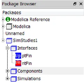
2.1.1 Pins
Pins are used as connectors in the Modelica language that take part nearly in all components when they are formed. The pins in the MSL are consisted of two variables, the potential at the pin, the voltage and its current.
For the mixed approach, the voltage and the carried current are time domain quantities and phasor domain quantities are needed to be defined in the pin model. The pins carry the information related to the complex quantities in the rectangular form. Given a pin labeled as “a” ,”a.Vre” stands for the real part of the complex potential, “a.Vim” stands for the imaginary part of the complex potential in the pin. “a.Ire” carries the information of the real part of the complex current which is a flow variable whereas “a.Iim” is the imaginary counterpart of the complex current. The time domain quantities of the MSL pin model are preserved in the mixed library pin model. In the end the modified pin model has six quantities compared with the MSL pin model which has two quantities.
Although the content of the pins are the same, two different pin models are coded for the approach, positive pin and negative pin.
Figure 2.4: Illustration of the Pins in the developed library
As we can see in figure 2.4 , positive pin is colored as blue and negative pin colored as red to distinct the connection in a clear way. A positive phasor and time domain pin is straightforwardly defined as:
connector ptPin "phasor or time domain positive pin"
SI.Voltage Vre "V phasor, real part";
SI.Voltage Vim "V phasor, imaginary part"; SI.Voltage v "v(t),time domain";
flow SI.Current Ire "I phasor, real part";
flow SI.Current Iim "I phasor, imaginary part"; flow SI.Current i "i(t),time domain";
end ptPin;
2.1.2 Sinusoidal Voltage Source
Electrical networks can be classified in the field of AC signals mostly due to the majority of the generated and transferred power is in AC signals excluding the renewable power supplies.
In order to mimic the alternating behavior of the signals, the circuits must be fed by sinusoidal sources. The MSL provides a sinusoidal voltage source model which has the path: Modelica.Electrical.Analog.Sources.SineVoltage. This component is capable of providing the time domain signals in sinusoidal fashion and can be used to express the time domain part of the proposed method inn the thesis. However the proposed mixed approach also relies on the adoption of the phasor domain equations whenever it is possible.
For the sake of achieving the task, the MSL component is modified to contain the phasor domain representation of the time domain signal in rectangular form.
A sinusoidal voltage signal in a component can be represented in different ways:
v(t) = A sin(ω t + φ) (2.1)
or
V = A˂φ (2.2)
where v(t) is the time domain voltage and V is the polar form of this voltage, ω stands for frequency, t for time, φ for phase of the signal.
The signals in the system which have this nature, also have a constant frequency and can be represented in this manner only when the system is at (sinusoidal) steady-state.
Given the specification of the phase, amplitude and frequency of the signal, the modified sinusoidal voltage source is introducing the time domain voltage and current as well as the real and imaginary parts of the complex voltage and current at its pins. The complex voltage and drawn current are always active and derived from the specifications of the time domain signal.
Figure 2.5: Symbol of sinusoidal voltage source
The computational efficiency is planned to be increased. The found solution makes use of this phenomenon; if the quantity to be derived is set to a constant somehow, the simulator will handle a deferential equation as an algebraic equation. This method, completely goes along with the very motivation of the methodology since solving algebraic equations are much more cost friendly than solving differential equations.
For the sake of simplicity, the choice of this constant is zero. Since the electrical components are not allowed to be put into simulation without the existence of a voltage/current source even in the MSL, the suggested guideline is compatible with the language itself. As a consequence of the voltages and currents are set to zero in the sources, the components with differential equations that have a connection with the sources, eventually discharge to zero eventually since for the components' perspective, it is equivalent to the task of grounding the component.
Practically speaking, as the cancellation of the time domain equations are explained, the logic behind switching of domains can be explained. As time domain switches to phasor domain, the transition is very straightforward. Since the phasor equations are always active, only the representation of the sinusoidal signal changes while killing the time domain equations. The transformation is shown as;
v(t) = A sin(ω t + φ) → V = A< φ (2.3) As can be seen from the relation, in polar form the dependency on time is hidden, and both formulas actually represent the same sinusoidal signal as long as frequency kept constant. That is the reason why frequency must be a fix value for continuity of the phasor domain. As stated earlier, the pins contain this relation in the rectangular form for the sake of utilization of the Kirchhoff's laws thus there is an addition transformation from polar form to rectangular form.
All the expressions in the equation 2.3 are actually the representations of the same sinusoidal signal. On the other hand, as phasor domain switches to time domain, the time domain equations are activated again.
Considering they are out of phase with the phasor domain equations at the time transition is requested -because they were already diminished to zero - the
action of re-initialization of the time domain equations based on phasor domain equations is required .
Thus, this voltage generator requires an additional input for the status of domain. At this release of the mixed library, the offset and starting time of the signal specifications are not implemented. The nucleus code of the component, Sine Voltage, is given below:
model SineVoltage "a source that provides sine voltage"
parameter Modelica.SIunits.Voltage Volt = 1 "Amplitude of sine wave"; parameter Modelica.SIunits.Angle phase = 0 "Phase of sine wave"; outer Modelica.SIunits.Frequency freqHz;
outer discrete Boolean TimeDom;
protected
constant Real pi = Modelica.Constants.pi; equation
0=a.Ire+b.Ire "KCL for real part of the complex current";
0=a.Iim+b.Iim"KCL for imaginary part of the complex current ";
cos(phase)*Volt=a.Vre-b.Vre" Real part of the complex voltage drop over the pins "; sin(phase)*Volt=a.Vim-b.Vim"Imaginary part of the complex voltage drop over the pins";
0 = a.i + b.i "KCL for time domain current ";
if TimeDom then
a.v-b.v=Volt* Modelica.Math.sin (2 * pi * freqHz * time + phase) " Time domain voltage drop if phasor domain cannot be utilized ";
else
a.v-b.v=0 " Time domain voltage drop if phasor domain cannot be utilized "; end if;
end SineVoltage;
Listing 2.5: sinusoidal voltage source
Resistor is one of the fundamental components of any electrical network. The voltage drops are calculated by using the resistance or the impedance with the corresponding currents. In the time domain the linear resistor has the relation:
vResistor (t) = iResistor (t) R (2.4)
Equation 2.4 is included in the resistor model of MSL and expresses the electrical relation between the pins of the resistor in the time domain.
Figure 2.6: Symbol of resistor
In the Mixed Library, the resistor model is modified to contain the impedance relation. Resistor is a passive component which does not change the phase difference between the voltage and the current across its' pins. The phase difference introduced by the resistor in the polar representation is zero. The impedance relations across the pins of the resistor can be written as:
V <θ = I < θ ZResistor <0° (2.5) Since the information of the complex current is available at the pins of the resistor.The phase of the complex current is summed with 0°. so it is equal to the phase of the complex voltage and amplitude of complex Voltage equals to the
multiplication of the impedance’s amplitudes and the complex current. The code of the resistor in the mixed library is given as:
model Resistor "Resistor for both time domain and phasor approaches"
parameter Modelica.SIunits.Resistance R = 1 "Resistance";
equation
0 = a . i + b . i "KCL for time domain current " ;
0 = a . Ire + b . Ire "KCL for real part of complex current " ; 0 = a .Iim + b .Iim "KCL for imaginary part of complex current " ; a . i *R = a .v - b.v " voltage drop relation in time domain " ;
R* sqrt ( a . Ire ^2+a .Iim ^ 2)*cos ( Modelica .Math.atan2 ( a .Iim , a . Ire ) )= a .Vr e - b.Vre " Real p a r t o f complex v o lt a g e drop " ;
R* sqrt ( a . Ir e ^2+a .Iim ^ 2)*sin( Modelica .Math.atan2 ( a .Iim , a . Ire ) )=a.Vim - b.Vim " Imaginary part of complex voltage drop " ;
Listing 2.6: Resistor
The output must be converted into rectangular form since the complex quantities on the pins have rectangular representation.
The proposed resistor model only needs the resistance value as an input and there is no need for a conditional statement in the resistor model because as anticipated in 2.5, the decaying of the time domain equations to zero is performed implicitly by setting the voltages to zero in the sources. Time and phasor domainequations are calculated at the same time during the whole simulation.
2.3. Capacitor
The motivation of this methodology relies on canceling the calculation of the differential equations so the MSL capacitor needs to be modified in a way that
the differential equations are replaced by impedance equations. The electrical relation can be expressed in time and phasor domain as in the equation 2.6 and 2.7 respectively .
icapacitor (t) = C 𝑑𝑣 𝑐𝑎𝑝𝑎𝑐𝑖𝑡𝑜𝑟
𝑑𝑡 (2.6)
VCapacitor < (θ - 90°) = Icapacitor < θ Zcapacitor < -90° (2.7)
Keep in mind that the impedance relation has a multiplicative nature, it is best to express it in the polar form.
Figure 2.7: Symbol of resistor
With the transformation from polar form to rectangular representation and the radian conversion, equation 4.5 can be coded in the Modelica language as follows:
0 = a.i + b.i;
a.i = Capacitance*der(v); 0=a.Ire+b.Ire;
0=a.Iim+b.Iim;
1/(Capacitance*C.freqHz*2*Modelica.Constants.pi)*sqrt(a.Ire^2+a.Iim^2)*cos (Modelica.Math.atan2(a.Iim,a.Ire)-Modelica.Constants.pi/2)= a.Vre - b.Vre ; 1/(Capacitance*C.freqHz*2*Modelica.Constants.pi)*sqrt(a.Ire^2+a.Iim^2)*sin( Modelica.Math.atan2(a.Iim,a.Ire)-Modelica.Constants.pi/2)= a.Vim - b.Vim ;
Listing 2.7: equations in capacitor in both domain
But, when dealing with the differential equations, the initial values of the equations must be known in order to integrate the equations correctly. The continuous time variable for the capacitor is the voltage in time domain. As long as the signal is purely sinusoidal ,the condition for the activation of the phasor domain, the time domain voltage drop across the pins of the capacitor can be expressed by the amplitude and the phase of the signal along with the internal clock of the simulator.
At the instant time domain is called, the initial value of the time domain voltage can be extracted from the phasor domain equations, and reinitialized with this value. The re-initialization action is performed every time the transition from phasor domain to time domain is requested. The capacitor requires the information regarding the choice of domain, thus the status of the domain choice is an input for the capacitor.
when all the capacitors are connected independently the system contain re-initialization clauses at the same number of capacitors. Capacitors may be dependent as in the case of parallel capacitors. When this is the case differential
algebraic index of the system is lower than re-initialization requests. This causes a syntax error for the compilers. Modelica compilers are not capable of adjusting themselves to deal with this problem automatically. So the user has to switch off the re-initialization part manually .The manual control of the re-initialization is performed by a Boolean flag called “ShallweInit”, which is also an input for the capacitor. The command “pre” stands for the previous value of variables before switching.
equation
if ShallWeInit then//”flag for enabling/disabling the use of initialization by user for the purpose of obeying DAE index restrictions”
when {TimeDom} then
reinit(v,sqrt(pre(a.Vim)^2+pre(a.Vre)^2+pre(b.Vre)^2+pre (b.Vim)^2-2*pre(a.Vim)*pre
(b.Vim)-2*pre(a.Vre)*pre(b.Vre))*sin(2*Modelica.Constants.pi*freqHz*time+Modelica .Math.atan2(pre(a.Vim)-pre(b.Vim),pre(a.Vre)-pre(b.Vre))));
end when;
when {dummy} then reinit(v,0);
end when; end if;
when time>0 then dummy=false;
end when;
Listing 2.8: code corresponds to the re-initialization process
Whenever the time domain is called, the time domain voltage at that instant is reconstructed based on the phasor domain data. The "dummy" variable is defiened in order to prevent the re-initialization at the beginning of the simulation.
In another word It guarantees the capacitor is reinitialized to zero instead of the data acquired from the phasor domain equations when time equals to zero. The "dummy" variable is not an input.
For the sake of summarizing the information up to now, in this proposed library the capacitor model contains the inputs of capacitance value, value of the utility frequency, status of the domain and the re-initialization flag.
However, for the implementation of switching operation between domains based on an event as anticipated, some additions are needed. Thus advanced switching method is realized in Mixed Library.
Nevertheless , a part of this method is coded in the capacitor model. Whenever the time domain is activated, for every second each capacitor counts the crossovers of the derivative of their voltages. The number of crossovers is equal to the frequency of the capacitor. If this calculated frequency of the capacitor is equal to the utility frequency in the system or in a admitted tolerance the corresponding capacitor sends a token which can be interpreted as a vote to a decision maker which named supervisor in this approach. if the complete agreement is guaranteed , the phasor domain can be initiated.
algorithm
when {der(v)<0 and TimeDom} then counter:=counter + 1;
end when;
when sample(0,1) then t:=max(counter); counter:=0;
end when;
if ((t>0) and
(t>=1.005*freqHz or t<=0.995*freqHz)) then s:=1;
end if;
(t<1.005*freqHz and t>0.995*freqHz) then s:=0;
end if;
Listing 2.9: advance switching method for capacitor based on frequency detection
Each second, the number of crossovers is counted by the variable “counter”, and at the end of one second the maximum number of crossovers is stored in variable “t”, Depending on the comparison of the capacitor's frequency with the utility frequency, the variable “s” takes the value of “1” or “0” (token which will be sent to the supervisor component to be analyzed.)
Although in this way computational burden would be increased when timedomain is activated with MSL capacitor. Hence to the differential equation, the component is required to count the crossovers of the time domain voltage which allocates more memory. Depending on the value of the utility frequency, the efficiency will be changed.
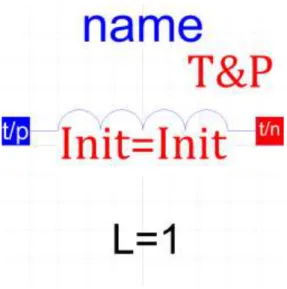
2.3. Inductor
Again like a capacitor, inductor is going to be modified with the same motivation.The inductance value, frequency, status of the domain, re-initialization flag, and the number of the inductors are inputs for the inductor .
Figure 2.8: Symbol of resistor
In time domain and phasor domain the inductor has the relation which expressed in 2.8 and 2.9 respectively:
vinductor (t) = L 𝑑𝑖 𝑐𝑎𝑝𝑎𝑐𝑖𝑡𝑜𝑟𝑑𝑡 (2.8)
Vinductor < (θ + 90°) = IInductor < θ ZInductor < 90° (2.9) The inductor introduces a positive phase shift of 90°. The time domain equations and the phasor domain equations with the corresponding polar to rectangular form transformation is coded as follows:
v = a.v - b.v;
0 = a.i + b.i;
a.v - b.v = L*
der
(a.i)
"inductor time domain "
;
0=a.Ire+b.Ire;
0=a.Iim+b.Iim;
(L*freqHz*2*Modelica.Constants.pi)*
sqrt
(a.Ire^2+a.Iim^2)*
cos
(
Mod
elica.Math.atan2
(a.Iim,a.Ire)+Modelica.Constants.pi/2)=
a.Vre-b.Vre;
(L*freqHz*2*Modelica.Constants.pi)*
sqrt
(a.Ire^2+a.Iim^2)*
sin
(
Mod
elica.Math.atan2
(a.Iim,a.Ire)+Modelica.Constants.pi/2)=
a.Vim-
b.Vim;
Listing 2.10: voltage-current relation in inductor expressed in modelica
And again here the re-initialization introduced below same as capacitor but for inductor the free variable is current. And as mentioned before in the capacitor case due to topology of the network inductors can also be dependent. So again the user must disable the re-initialization to prevent the error.
if ShallWeInit then
when {TimeDom} then
reinit(a.i,sqrt(pre(a.Iim)^2+pre(a.Ire)^2)*sin(2*Modelica.Constants.pi*freqHz*time+Modelic a.Math.atan2(pre(a.Iim),pre(a.Ire))));
end when;
when {dummy} then reinit(a.i,0);
end when; end if;
Listing 2.11: re-initialization of inductor’s current in time domain
Again an algorithm is developed for the implementation of the advanced switching method.
algorithm
when {der(a.i)<0 and TimeDom} then counter:=counter + 1;
end when;
when sample(0,1) then t:=max(counter);
counter:=0; end when;
if ((t>0) and
(t>=1.005*freqHz or t<=0.995*freqHz)) then s:=1;
end if;
if (t>0) and
(t<1.005*freqHz and t>0.995*freqHz) then s:=0;
end if;
Listing 2.12: advance switching method for inductor based on frequency detection
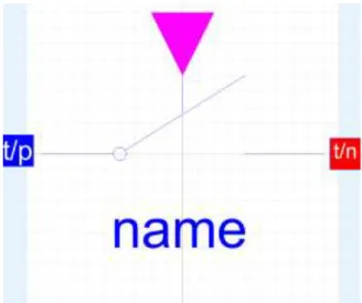
2.4. Ideal opening and closing switch
The switching behavior is controlled by input signal control. For the opening switch if control is true then pin a is not connected with negative pin b. Otherwise, pin a is connected with negative pin b.
Figure 2.9: Symbol of Ideal opening/closing switch
During the switching action, the opened switch has a very low conductance Goff and the closed switch has a very low resistance Ron. Both the conductance
and the resistance are 1e-5 by default, but these parameters can be changed based on the design. For simplicity, the heat dependency of the parameters is ignored.
equation a.i+b.i=0;
a.v-b.v = (s1*unitCurrent)*(if control then 1 else Ron); a.i = (s1*unitVoltage)*(if control then Goff else 1); 0=a.Ire+b.Ire;
0=a.Iim+b.Iim;
a.Vre-b.Vre=(s2*unitCurrent)*(if control then 1 else Ron); a.Vim-b.Vim=(s3*unitCurrent)*(if control then 1 else Ron); a.Ire=(s2*unitVoltage)*(if control then Goff else 1);
a.Iim=(s3*unitVoltage)*(if control then Goff else 1);
Listing 2.13: Ideal opening and closing switch
A physical event that can initiate the transition between domains. It is possible to execute the transitions between domains on an event based way instead of switching defined on the system level where the switching is requested based on time.
When the generators are connected, which means the switches are closed, the system is simulated in the time domain. At this version of the presented library, whenever a single generator is connected to the network, the whole system is simulated in the time domain.
For the case of opening switch, whenever the control signal is false the system goes into the time domain and stays in the time domain as long as the control signal is false.
The vectors of the time varying components and the switches are summed together, the unanimity is preserved for switching back to phasor domain, even only once switch is sending a time domain flag, entire system operates in the
time domain. Whenever the control signal is true, the synchronization methods can be applied for switching back to phasor domain.
algorithm
when control==true then L:=0;
end when;
when control==false then L:=1;
end when;
Listing 2.14: vote of the switch
2.5. Transformers
The transformer model takes three inductance inputs: two for the main inductances and one for the coupling one. This component has two different currents following through. the transformer takes also the utility frequency and the status of the domain as inputs.
parameter SI.Inductance L1(start=1) "Primary inductance"; parameter SI.Inductance L2(start=1) "Secondary inductance"; parameter SI.Inductance M(start=1) "Coupling inductance"; 0 = a1.i + b1.i; 0=a1.Ire+b1.Ire; 0=a1.Iim+b1.Iim; 0 = a2.i + b2.i; 0=a2.Ire+b2.Ire; 0=a2.Iim+b2.Iim; //v1=a1.v-b1.v; //v2=a2.v-b2.v;
a1.v-b1.v = L1*der(a1.i) + M*der(a2.i); a2.v-b2.v = M*der(a1.i) + L2*der(a2.i);
(L1*C1.freqHz*2*Modelica.Constants.pi)*sqrt(a1.Ire^2+a1.Iim^2)*cos(Modelica.Math.atan 2(a1.Iim,a1.Ire)+Modelica.Constants.pi/2) + (M*C1.freqHz*2*Modelica.Constants.pi)*sqrt(a
2.Ire^2+a2.Iim^2)*cos(Modelica.Math.atan2(a2.Iim,a2.Ire)+Modelica.Constants.pi/2)= a1.Vre-b1.Vre ; (L1*C1.freqHz*2*Modelica.Constants.pi)*sqrt(a1.Ire^2+a1.Iim^2)*sin(Modelica.Math.atan2 (a1.Iim,a1.Ire)+Modelica.Constants.pi/2) + (M*C1.freqHz*2*Modelica.Constants.pi)*sqrt(a2 .Ire^2+a2.Iim^2)*sin(Modelica.Math.atan2(a2.Iim,a2.Ire)+Modelica.Constants.pi/2)= a1.Vim-b1.Vim; (M*C2.freqHz*2*Modelica.Constants.pi)*sqrt(a1.Ire^2+a1.Iim^2)*cos(Modelica.Math.atan2 (a1.Iim,a1.Ire)+Modelica.Constants.pi/2) + (L2*C2.freqHz*2*Modelica.Constants.pi)*sqrt(a 2.Ire^2+a2.Iim^2)*cos(Modelica.Math.atan2(a2.Iim,a2.Ire)+Modelica.Constants.pi/2)= a2.Vre-b2.Vre; (M*C2.freqHz*2*Modelica.Constants.pi)*sqrt(a1.Ire^2+a1.Iim^2)*sin(Modelica.Math.atan2 (a1.Iim,a1.Ire)+Modelica.Constants.pi/2) + (L2*C2.freqHz*2*Modelica.Constants.pi)*sqrt(a 2.Ire^2+a2.Iim^2)*sin(Modelica.Math.atan2(a2.Iim,a2.Ire)+Modelica.Constants.pi/2)= a2.Vim-b2.Vim;
Listing 2.15: The time domain and the phasor domain relationships
The code above expresses the basic transformer model in mixed approach. The ideal transformer has another input (n) in order to defined the turns ratio between primary and secondary winding. The code in developed library for this purpose as:
a1.v-b1.v = n*(a2.v-b2.v);
a1.Vre-b1.Vre=n*(a2.Vre-b2.Vre); a1.Vim-b1.Vim=n*(a2.Vim-b2.Vim);
Figure 2.10: Symbol of Ideal transformer
2.5. The supervisor
The role of the supervisor is to take decisions on which mode to be utilized, by considering the the information which is received from the components. It creates a link between the components and status of the domain which is an input for the involved components.
The link between the components and the supervisor is constructed by using the “inner” and “outer” clauses of the Modelica language. Its variables are
coded with the “inner’ command, whereas all the components including
the supervisor take place under the model and their variables are coded
with the “outer” command.
An code written on the “parent” model can be given:
inner Real S [ 4 ] " Switch vector " ;
inner Real R[ 24 ] " Vector of Capacitors and Inductors " ;
inner Modelica.SIunits.Frequency freq Hz = 50 " Utility frequency system " ;
inner discrete Boolean TimeDom( s t a r t =f a l s e ) " Value of this parameter is set on the component , Supervisor " ;
Listing 2.16: the supervisor in developed library
The switches, capacitors and inductors send data to the model. These sent data can be considered as votes for the domain change.The votes can either be
“0” or “1” for every component that has the privilege to vote. “0” votes stand for the request of phasor domain and “1” votes stand for the request of time domain.
when sum of the votes equal to zero,it means that there is no request of time domain, then the system can operate under the phasor mode. In contrary as long as one of the components send the request of time domain, thus the system operates under the time domain.
for i in 1:n loop Sum:=R[i]+Sum; end for; for j in 1:m loop Sum2:=S[j] + Sum2; end for; Sum:=Sum+Sum2; t:=max(Sum); Sum:=0; Sum2:=0; if t>0 then TimeDom:=true; else TimeDom:=false; end if; if time<=3 then TimeDom:=true; end if;
Listing 2.17: decision made by supervisor based on status of switches and components
By bringing the last “if” , it guarantees to start in the time domain at the beginning of the simulation.
Chapter 3
Simulation Examples
This chapter reports and discusses some simulation results, evidencing the obtained advantages with respect to a purely time-domain modelling context, and also depending some operating condition boundary that actually makes the presented approach advantageous.
The components of MSL can be expected to function optimally and any modification to MSL puts more computational burden to the compiler. With the introduction of conditional loops, the simulations with modified components become slower. Moreover, when the system operates under the time domain, capacitors and inductors perform derivation operations on either voltage or current values respectively.
The most visible reflection of this phenomenon is on the number of the Jacobian evaluations;with the excessive use of time domain the number of Jacobian evaluations is expected to be much higher than its MSL counterpart.
Due to the inefficiency of the components coded according to the mixed approach in the time domain, the feasibility of the application of the mixed approach is questionable under some conditions. If the time domain is requested for a large portion of the simulation time, the usage of the MSL components is clearly preferable. It is the genuine task of identifying the conditions where mixed approach becomes advantageous over MSL.
In order to validate the mixed approach in the sense of performance, two examples are presented. The examples are prepared to reflect real networks thus the approach can be evaluated realistically.
An illustrative simulation example
We now shows a simple simulation example to demonstrate the operation of the
proposed modelling framework, and specifically of the changeover management
.
The example refers to the small network model depicted in Figure 5. The switch SW1 , initially closed, is opened at t = 1 s and re-closed at t = 2 s.Figure 3.1: basic simulation example
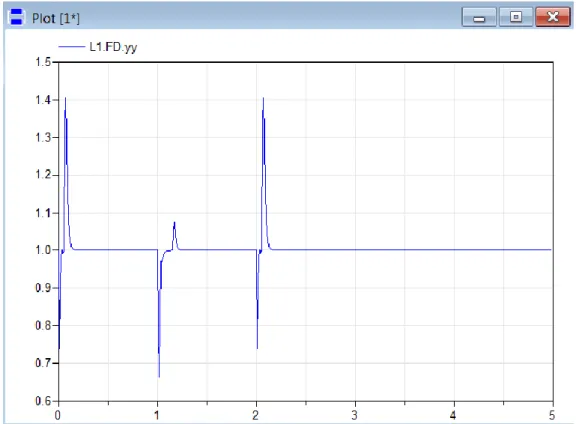
Figure 3.2 shows the yy(t) variables in the frequency detectors of the inductor. Recall that those variables are meant to indicate, by assuming a nearly constant unity value, the settling of the locally measured frequency to freqHz (here set to 50 Hz).
As can be seen, the expected effect is obtained, and the normalized nature of the involved signals produces comparable transients also in the presence of different values for the components’ electric parameters.
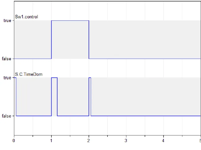
Figure 3.3: bolean flags
In Figure 3.3, the relevant Boolean flags at the system level are instead represented. The changeover mechanism catches the switch events, passing to time domain instantaneously, while the time domain periods are not equal, correctly depending on the transient behavior of the monitored electric variables.
Figure 3.4: forcing time domain on the part of a switch
Figure 3.4 illustrates how a commuting component forces the transition to time domain mode by means of xsd and the role of the threshold and the time constant of its dynamics in determining the width of the generated pulse. Note that the rising edge of that pulse is structurally synchronous to the switch command, which is consistent with the defined specifications.
Figure 3.5: current in R1in time domain representation
Figure 3.6: current in R1 phasor representation.
Figures 3.5 and 3.6 show the behaviour of the current flowing through resistor R1, viewed respectively in the time domain and as a phasor (for which the real and the imaginary part are plotted). Notice that when the simulation switches back to phasor mode after a period in time domain mode triggered by a switch event,
Chapter 4
Conclusions
A Modelica library was presented to allow modeling an AC network in both the time and the phasor domain.A primary characteristic of the presented models is that the changeover between the two modes above is managed automatically, requiring a minimal effort on the part of the user.
This allows to deal with simulation studies where long periods of quasi-stationary operation are interspersed with abrupt events.Simulation examples show the correctness of the proposed approach, and its efficacy in terms of simulation speed improvement.
Future work will concern further extensions to the library, and in erspective, the integration of the presented mixed-mode modeling approach, and in particular of the changeover mechanism, into libraries coming from neighboring research lines, in a view to unifying efforts.
Bibliography
[1] R. Caldon, F. Rossetto, and R. Turri. Temporary islanded operation of dispersed generation on distribution networks. In Universities Power Engineering Conference, 2004. UPEC 2004. 39th International, volume 3, pages 987{991. IEEE, 2004.
[2] F. Casella and A. Leva. Modelling of thermo-hydraulic power generation processes using modelica. Mathematical and Computer Modelling of Dynamical Systems, 12(1):19{33, 2006.
[3] S. Mattsson, H. Elmqvist, and M. Otter. Physical system modeling
with Modelica. Control Engineering Practice, 6:501{510, 1998.
[4] G. Kariniotakis, N. Soultanis, A. Tsouchnikas, S. Papathanasiou,and N. D. Hatziargyriou. Dynamic modeling of microgrids. In Future Power Systems, 2005 International Conference on, pages 7-pp.IEEE, 2005.