A forecasting performance comparison of dynamic factor models based on static and dynamic methods

(1)

Research Article

Commun. Appl. Ind. Math. 8 (1), 2017, 43–66 DOI: 10.1515/caim-2017-0003

A forecasting performance comparison of dynamic

factor models based on static and dynamic

methods

Fabio Della Marra1_*

1_{Department of Economics, University of Parma, Parma, Italy.} *_{Email address for correspondence:}_{fabio.dellamarra@iispascal.it}

Communicated by Nicola Bellomo

Received on 12 14, 2016. Accepted on 02 16, 2017. Abstract

We present a comparison of the forecasting performances of three Dynamic Factor Models on a large monthly data panel of macroeconomic and financial time series for the UE economy. The first model relies on static principal-component and was introduced by Stock and Watson (2002a, b). The second is based on generalized principal components and it was introduced by Forni, Hallin, Lippi and Reichlin (2000, 2005). The last model has been recently proposed by Forni, Hallin, Lippi and Zaffaroni (2015, 2016). The data panel is split into two parts: the calibration sample, from February 1986 to December 2000, is used to select the most performing specification for each class of models in a in-sample environment, and the proper in-sample, from January 2001 to November 2015, is used to compare the performances of the selected models in an out-of-sample environment. The metholodogical approach is analogous to Forni, Giovannelli, Lippi and Soccorsi (2016), but also the size of the rolling window is empirically estimated in the calibration process to achieve more robustness. We find that, on the proper sample, the last model is the most performing for the Inflation. However, mixed evidencies appear over the proper sample for the Industrial Production.

Keywords: Macroeconomic Forecasting, Dynamic Factor Models, Time-domain methods, Frequency-domain methods

AMS subject classification: 62P20

1. Introduction

In this paper, a comparative analysis of the forecasting performance of three Large-Dimensional Dynamic Factor Models is presented. As a key feature, Dynamic Factor Models represent each variable in a dataset as the sum of two orthogonal terms: a common component χt, driven by a reduced

(as compared to the number of series in the dataset) number of common factors, and an idiosyncratic component ξt, which represents measurement

errors or local features. Among the different versions of the Dynamic Factor Models we selected:

(2)

(i) SW model. This time-domain method was introduced in [1], [2]. The factors are estimated by computing static principal components of the variables in the dataset. Let yit be the variable of the dataset to

be forecasted at time t, its h-step-ahead prediction equation (also called Diffusion Forecast Index ) is obtained by regressing yit+h on

the factors and on yit itself. Lags of the factors and of yit may be

added.

(ii) FHLR model. This frequency-domain method was proposed in [3], [4] and requires the computation of two steps. In a first step, the com-mon component χt, the idiosyncratic component ξtand their

covari-ances are estimated using a frequency-domain method introduced in [3] named Dynamic Principal Component. In the second step, the factors are estimated by computing Generalized Principal Compo-nents.

(iii) FHLZ model. This frequency-domain method was proposed in [5], [6]. Here, the underlying assumption in (i) and (ii) that the common components span a finite-dimensional space as n tends to infinity is relaxed. The estimation of the parameters is much more complex though.

There exists some literature comparing the forecasting performances of SW and FHLR, but universal consensus still does not seem to have been reached. Theoretically, time-domain methods consider only relations among the variables at the same time, whereas frequency-domain methods exploit leaded and lagged relations among the variables. However time-domain methods require less parameters to be calibrated. Hence they are more robust to misspecification than frequency-domain methods. Empiri-cally, in [7] Boivin and Ng found that SW generally outperforms FHLR on US macroeconomic data, whereas D’agostino and Giannone in [8] found no relevant differences in the performance of both methods on the whole sam-ple (even though heterogeneity is found in subsamsam-ples). In [9] Schumacher found that FHLR outperforms SW on the prediction of the German GDP. The same conclusions are drawn in [10] over the forecasting of Dutch GDP. So far, a systematic comparison of the forecasting performances of SW, FHLR and FHLZ can be found only in [11]. Here, Forni et al. conducted a forecasting exercise on an US macroeconomic dataset, where they took an autoregressive process of order 4 as a benchmark. They showed that FHLZ oupterforms SW, FHLR and the benchmark both for Industrial Produc-tion and InflaProduc-tion during the Great ModeraProduc-tion. In the Great Recession, the forecasting performances of the Industrial Production change dramat-ically: all factor models are outperformed by the benchmark and SW and

(3)

FHLR outperform FHLZ. Hence, Forni et al. concluded that, due to its more dynamical structure, FHLZ tends to be the best performing method in “stationary period”, but it loses ground during regime changes. Also, they showed that FHLZ tends to be outperforming on nominal variables and FHLR on real variables.

In this paper, a large macroeconomic dataset consisting of 176 EU macroeconomic and financial time series observed at monthly frequency over the period from February 1986 to November 2015 is used to anal-yse the forecasting performance of these methods. To achieve stationarity, the series are deseasonalized and transformed. No treatment for outliers is applied.

As in [11], the EU dataset is split into two subsamples. The former, from February 1986 to December 2000, will be used to calibrate the models, i.e. to produce in-sample forecasts of the variables of the EU dataset for several specifications of SW, FHLR and FHLZ. Then, for each class of models, we selected the specification which shows the minimum mean square forecast error (MSFE). These models are then run and compared in the remaining sample, from January 2001 to November 2015.

The paper is structured as follows. In Section 2, the factor models are discussed in detail. In Section 3, the main features of the dataset are illus-trated. In Section 4, the calibration process of the models is described. In Section 5, results are discussed and Section 6 concludes.

2. An overview on Dynamic Factor Models

Let {xt = (x1t ... xnt)0|t = 1, ..., T } be a n-dimensional vector of time

series, which will be denoted as xt for simplicity. xt will be assumed to

be weakly-stationary, purely non deterministic with zero mean and unit variance. Let us assume that the following decomposition holds:

(1) xt= χt+ ξt.

The process χt= (χ1t ... χnt)0 is called common component. It will be

assumed that χit is stationary and that χit is costationary with χjt for all

i, j = 1, ..., n such that i 6= j. The process ξt is called idiosyncratic

compo-nent. It will be assumed that ξit is stationary and that ξit is costationary

with ξjt for all i, j = 1, ..., n such that i 6= j. A distinction between static

and dynamic factor models can be made according to the functional form selected for the common component. In static factor models, the common component can be modeled as χt = ΛFt where Λ ∈ Rn×r is called the

(4)

t, with r << n. In dynamic factor models, the common component takes into account also the lags of the factors. Hence, the common component can be modeled as χt= Λ(L)ut. Here L is the lag operator, Λ(L) ∈ Rn×q

is called the factor-loading matrix and ut∈ Rqis the vector of the dynamic

factors at time t, with q << n. In [12], [13], it is shown that ut is a

or-thonormal white noise process. Moreover, fixed a maximum lag order s for the matrix Λ(L), a dynamic factor model can be rewritten as a static factor model by staking all of the factors with their lags in a single vector, i.e. by imposing Ft = (ut ... ut−s). More details can be found in [14]. This way,

it holds that r << q << n. The three different dynamic factor models for estimating the factors are discussed in the following subsections.

2.1. The SW model

In [1], [2], Stock and Watson proposed a static factor model whose components are estimated by means of static principal component. Let ˆ

Γ = T−1PT

t=1xtx 0

t be the sample covariance matrix of xt. By computing

the eigenvalues of ˆΓ and stacking them into the matrix P = (P₁ ... Pr)0,

with Pi the eigenvector corresponding to the i-th largest eigenvalue, we can

compute the factors ˆFt= P0xt The h-step ahead SW forecasting equation,

also called Diffusion Forecast Index, can be computed by regressing xit+h

on the factors ˆFt and xit. Lags of both ˆFt and xit may be added. Hence,

the Diffusion Forecast Index can be modeled as

(2) xit+h|t = ai(L)ˆFt+ bi(L)xit,

where ai(L) is a n × r vector of polynomials of degree αi and bi(L) is a

scalar polynomial of degree βi.

2.2. The FHLR model

This model was proposed by Forni et al. in [3], [4]. It is articulated in two steps:

(i) Estimation of the common and idiosyncratic component : let ˆΓ(k) = T−1PT

t=1xtx0_t−k be the sample autocovariance of xt at lag k.

In order to consistently estimate the spectral density matrix of xt, we can compute this estimator ˆΣ(θ) = Pdt=−dwkΓ(k)eˆ −ikθ

with wk being the weights of a kernel function. By computing

the spectral decomposition of ˆΣ(θ) for all θ, the spectral density matrix of the common component can be reconstructed by com-puting ˆΣχ(θ) = ˆP(θ)Λ(θ) ˆP∗(θ), where Λ(θ) denotes the

(5)

ˆ

P(θ) = ( ˆP₁(θ) ... ˆPq(θ)) the matrix whose columns are the

corre-sponding eigenvectors. The spectral density matrix of the idiosyn-cratic component can be reconstructed by differencing ˆΣξ(θ) =

ˆ

Σ(θ) − ˆΣχ(θ) Autocovariances at lag k of the common and the

idiosyncratic component can be obtained by computing the inverse Fourier transform of their estimated spectral density matrix. (ii) Estimation of the factors: now, the estimated covariance matrix of the

common component and of the idiosyncratic component are used to solve the generalized principal components problem:

(3) Σˆ0_ξP = ˆΣ0_χPD,

s.t. P0Σˆχ 0

P = I, where D is a diagonal matrix whose entries are the r largest eigenvalues of the pair ( ˆΣ0

ξ, ˆΣ0χ) and P is the matrix

containing the corresponding eigenvectors. The first r factors are defined as ˆFt= P0xt

By means of the projections:

ˆ

χ_it+h|t= P roj[χit+h|ˆFt]

ˆ

ξit+h|t= P roj[ξit+h|xit ... xit−p],

(4)

the h-step ahead FHLR forecasting equation can be finally derived as

(5) χ_it+h|t = ˆχ_it+h|t+ ˆξ_it+h|t. 2.3. The FHLZ model

This model was proposed by Forni et al. in [5], [6]. Differently from the previous models, here the assumption that the common component spans a finite-dimensional space is relaxed. This model is articulated in the steps listed below:

(i) Estimation of the spectral density matrix ˆΣx(θ) of xt: the

spec-tral density matrix Σˆx(θ) can be estimated as Σˆx(θ) =

1 2π

PR

k=−RωkΓ(k)eˆ −ikθ with ωkrepresenting the weights of a kernel

function.

(ii) Estimation of the spectral density matrix ˆΣχ(θ) of χt: it is obtained

by computing the dynamic principal components of ˆΣx(θ) and then by selecting its q principal components which are associated to the largest eigenvalues. For more details, see [3], [5].

(6)

(iii) Estimation of the autocovariance matrices ˆΓχ_k of χt: The

autocovari-ances of χtare estimated by means of the Wiener-Khinchin-Einstein

theorem.

(iv) Estimation of the VAR matrices ˆAk_{(L): under general assumptions,}

the common component admits a unique blockwise autoregressive representation of the form:

(6)         A1(L) 0 . . . 0 . . . 0 A2(L) . . . 0 . . . .. . ... . .. 0 0 . . . Ak(L) . . . .. . . ..         χt=         R1 R2 .. . Rk .. .         ut,

where Ak(L) ∈ R(q+1)×(q+1) is a polynomial matrix of finite de-gree and Rk∈ R(q+1)×q_{. To estimate the VAR matrices A}k_{(L), the}

covariances ˆΣχ(θ) are employed.

(v) Estimation of the matrices Rkand the shock ut: these estimates can be

recovered by applying standard principal components to the process A(L)xt.

By inverting equation (6) it follows that: χt = [A(L)−1]Rut =

C(L)ut= C0ut+ C1ut−1+ ... where ˆχt∈ Rnand ˆA(L), ˆR, ˆW(L) ∈ Rn×n.

The h-step ahead FHLZ forecasting equation is reported below:

(7) χ_it+h|t= Chut+ Ch+1ut−1+ ... .

3. Description of the dataset

In this empirical application, a large macroeconomic dataset consisting of 176 EU macroeconomic and financial time series observed at monthly frequency is employed. This dataset contains real variables (import/export price indexes, employment, Industrial Production) and nominal variables (money aggregates, consumer price indexes, wages), asset prices (stock prices and exchange rates) and surveys. Further details can be found in the Appendix. To achieve stationarity, several series are deseasonalized and transformed. No treatment for outliers is applied. In addition to SW, FHLR, FHLZ, the forecasts of an autoregressive process (AR) of order 4 are com-puted. The dataset is divided in two parts: a calibration sample, ranging from February 1986 to December 2000, which will be employed to select the most performing specification of each model, and a proper sample, ranging

(7)

from January 2001 to November 2015, which will be employed to compare the selected specifications of each model. As in [2], [8], to assess the forecast-ing performances, the variables which are taken into account are the level of the logarithm of the Industrial Production (IP) and the yearly change of the logarithm of the Consumer Price Index (CPI). Forecasts are computed h-months ahead, with h ∈ {1, 3, 6, 12, 24}. For each methods, we employed a rolling-window scheme [t − l, t], whose size l will be determined in the calibration sample. To assess the forecasting performance of each model, the mean-square forecast error (MSFE) is employed as a metric:

(8) M SF Eh(i) = 1 (Tend− h) − Tbegin+ 1 Tend−h X k=Tbegin SF E_kh(i),

where Tbegin, Tend stand, respectively, for the first and the last date in

the dataset and i ∈ {SW, F HLR, F HLZ, AR}. SF Eh _{stands for h-step}

ahead squared forecast error and is defined as SF Eh(i) = (y_t+h|Ti − yt+h)2,

where y_t+h|Ti is the forecasted value at horizon h of the variable yt by the

method i and yt+h is its real value.

4. Calibration

The calibration procedure is basically the same as in [11], but is more robust since the size of the rolling window is taken into account as a param-eter to be tuned. The calibration sample, ranging from February 1986 to December 2000, will be used to calibrate the methods SW, FHLR, FHLZ. Namely, this portion of the dataset will be used to select the best performing specifications of each class of models. To compare the performances of two different methods, say α, β, at a certain horizon h, the ratio mean-square forecast error (RMSFE) will be computed. Such metric is defined as

(9) RM SF Eh(α, β) = M SF E

h_(α)

M SF Eh_(β) .

4.1. Calibration of SW

To produce forecastings by means of equation (2), the following param-eters must be calibrated:

(i) the number of static factors r: ranging from 1 to 10. Also, a comparison with Bai & Ng criterium (BN) with maximum 12 factors has been made.

(8)

(ii) the degree α of a(L): ranging from 1 to 10. (iii) the degree β of b(L): ranging from 0 to 10.

(iv) the size l of the rolling window : ranging from 5 to 12 years.

By selecting the values of the parameters which guarantee the lowest mean RMSFE, the chosen configuration for the IP is the following:

(10) (r, α, β, l) = (4, 1, 0, 7).

Instead, the chosen configuration for the CPI is the following:

(11) (r, α, β, l) = (4, 1, 9, 12).

4.2. Calibration of FHLR

(i) the number of static factors r: ranging from 1 to 10. Also, a comparison with Bai & Ng criterium (BN) with maximum 12 factors has been carried out.

(ii) the number of dynamic factors q: ranging from 0 to 10. Also, a com-parison with Hallin-Liska criterium (HL) with maximum 12 factors has been carried out.

(iii) the type of kernel k: ranging in the set {Triangular, Rectangular, Parzen, Gaussian, Exponential, Cosine, Tukey, Hann}.

(iv) The lag window d for spectral density estimation: ranging in the set {25, 35, 40}.

(v) the size l of the rolling window : ranging from 5 to 12 years.

(12) (r, q, k, d, l) = (4, 3, T ukey, 25, 12).

(9)

4.3. Calibration of FHLZ

(i) the number of dynamic factors q: ranging from 1 to 5. Also, a compar-ison with Hallin-Liska criterium has been carried out.

(ii) the type of kernel k: ranging in the set {Triangular, Rectangular, Parzen, Gaussian, Exponential, Cosine, Tukey, Hann}.

(iii) the lag window d for spectral density estimation: ranging in the set {25, 35, 40}.

(iv) the maximum lag ml for the matrix Ak(L): ranging from 1 to 5. (v) the size l of the rolling window : ranging from 5 to 12 years.

(14) (r, k, d, ml, l) = (4, P arzen, 25, 4, 12).

(15) (r, k, d, ml, l) = (2, Rectangular, 25, 1, 7).

5. Results on the proper sample

5.1. Prediction of the Industrial Production and the Inflation

Now, the forecasting performances of the three dynamic factor models over the IP and CPI are compared on the proper sample, which starts on January 2001 and ends on November 2015. To forecast the IP, we changed the size of the rolling window employed in SW from 7 to 12 years. Instead, to forecast the CPI, we changed the size of the rolling window employed in SW from 12 to 7 years. Hence, to forecast the IP and the CPI, all dynamic factor models employ a rolling window of the same length. The common benchmark for the factor models is the autoregressive process (AR) of order four. In table 1, the average RMSFEs (relative to the AR) of the selected dynamic factor models are reported for the IP and CPI on the whole proper sample. However, as reported by CEPR, during the proper sample, the eu-ropean economy faces two crisis periods: the first starts on May 2008 and ends on January 2009. The second starts on September 2011 and ends on March 2013. Hence, it is reasonable to assess whether the relative forecast-ing performances of the three dynamic factor models present a relevant

(10)

change during the crisis periods. In table 2, the average RMSFEs (relative to the AR) of the three dynamic factor models are reported for the IP and the CPI from January 2001 to April 2008 (i.e. before the first crisis on the proper sample). In table 3, the average RMSFEs (relative to the AR) of the three dynamic factor models are reported for the IP and the CPI from January 2001 to August 2011 (i.e. before the second crisis on the evaluation sample). One, two or three asterisks indicate that the null of equal perfor-mance of the three factor models relative to AR is rejected at, respectively, the 1%, 5%, 10% significance by the Giacomini-White Test. One, two or three daggers indicate that the null of equal performance of FHLR, FHLZ relative to SW is rejected at, respectively, the 1%, 5%, 10% significance by the Giacomini-White Test. For further details about Giacomini-White Test, see [15].

Table 1. RMSFEs on the whole sample: IP on the left, CPI on the right. IP CPI h/model F HLZ F HLR SW F HLZ F HLR SW 1 0.97 0.95 0.92 0.95 1.01 1.17 3 0.84 0.82 0.82 0.88∗∗∗ 0.95 1.08 6 0.66 0.66 0.68 0.85 0.94 1.04 12 0.80 0.81 0.79 0.85 0.87 1.18 24 0.94 0.94 0.92 1.02 1.02 1.47

Table 2. RMSFEs from January 2001 to April 2008: IP on the left, CPI on the right. IP CPI h/model F HLZ F HLR SW F HLZ F HLR SW 1 1.15 1.20 1.24 0.96 0.98 0.99∗∗∗ 3 0.80 0.82 0.79 1.05 1.07 1.14 6 0.92 1.03 1.15 1.14∗∗† 1.17∗∗†† 1.32∗ 12 0.91 1.03 1.03 1.00∗∗∗† 1.04∗∗†† 1.32∗ 24 0.85 0.84∗ 0.86∗ 0.79 0.82 1.09

The relative performances of all methods tend to improve especially after the first crisis at horizons h ∈ {1, 3, 6, 12}. This holds both for IP and CPI. This is also illustrated in figure 1 (on the left), in which the graphs of the cumulated sums of the square forecast error at h = 6 for the IP are reported. The corresponding plots are similar for different values of h 6= 24 and are not reported here. The shaded areas correspond to the two crisis periods in the proper sample, according to CEPR. A relevant jump can be observed during the first crisis for all methods, including the benchmark, followed by a period of permanent flatness. However, after the first crisis,

(11)

Table 3. RMSFEs January 2001 to August 2011: IP on the left, CPI on the right.

IP CPI h/model F HLZ F HLR SW F HLZ F HLR SW 1 0.95 0.87 0.82 0.97 1.06 1.24 3 0.84 0.77 0.78 0.90 0.97 1.08 6 0.65 0.65 0.66 0.85 0.92 0.97 12 0.79 0.80 0.76 0.85 0.87 1.11 24 0.98 0.98 0.93 1.24 1.23 1.82

the sum of the cumulative forecast errors of AR increases substantially in comparison with those of the dynamic factor models (e.g., on October 2009, the sum of the cumulative forecast errors of AR increases, on average, more than 50% in comparison with those of the dynamic factor models). Similar results are obtained for the CPI and are not reported here.

01-02 01-04 01-06 01-08 01-10 01-12 01-14 Time 0 1 2 3 4 5 6 7 8 9 Forecast error #10-3 FHLZ FHLR SW AR 01-04 01-06 01-08 01-10 01-12 01-14 Time 0 0.2 0.4 0.6 0.8 1 1.2 1.4 1.6 1.8 2 Forecast error #10-3 FHLZ FHLR SW AR

Figure 1. Cumulative sum of the square forecast error at h = 6 for the IP (on the left). Cumulative sum of the square forecast error at h = 24 for the IP (on the right).

Instead, at horizon h = 24, the relative performances of all methods tend to worsen after the first crisis. This is also illustrated in figure 1 (on the right), in which the graph of the cumulated sums of the square forecast error for the IP are reported. In this plot, a jump during the first crisis can be obeserved whose slope is less remarked than in the left-side plot. This behaviour seems to persist until the beginning of the second crisis, after which a period of permanent flatness arises. However, no substantial increase in the sum of the cumulative forecast errors of AR appears in comparison with the dynamic factor models. Similar results are obtained for the CPI and are not reported here.

As in [11], to assess the forecasting performance of each couple of meth-ods locally, each time series of the dataset is smoothed by a centered moving

(12)

average of length m = 61 (with coefficients equal to 1/m) and then the Fluc-tuation test ( [16]) is run, at 5% significance level. The results for the IP at horizons h ∈ {6, 12, 24} are reported in Figure 2. All methods outperform AR significatively from the first crisis on. At horizon h = 6, FHLR and FHLZ outperforms SW on average on the whole sample, except during the first crisis. Instead, at horizons h ∈ {12, 24}, SW outperforms FHLR and FHLZ from the first crisis on. FHLR tends to outperform FHLZ in the two crisis periods. Outside the crisis periods, FHLZ tends, on average, to out-perfom FHLR at horizons h ∈ {6, 12}. Instead, at horizon h = 24, FHLR outperforms FHLZ from the first crisis on.

The results for the CPI at horizons h ∈ {6, 12, 24} are reported in Figure 3. FHLR and FHLZ tend to outperfom SW at all horizons, except FHLR at horizon h = 6 during the former crisis.

FHLR and FHLZ tend to outperfom SW at all horizons, except FHLR at horizon h = 6 during the first crisis. FHLR and FHLZ outperform AR at horizons h ∈ {6, 12}. At horizon h = 24, AR outperforms FHLR and FHLZ from the first crisis on. SW outperforms AR during the two crisis periods at horizons h ∈ {6, 12}. At horizons h ∈ {12, 24}, AR outperforms SW from the second crisis on. At all horizons, FHLZ outperforms FHLR during the first crisis. At horizons h ∈ {6, 12}, this behaviour seems to be permanent. Instead, at horizon h = 24, FHLR outperforms FHLZ from the second crisis on.

5.2. Prediction of the dataset

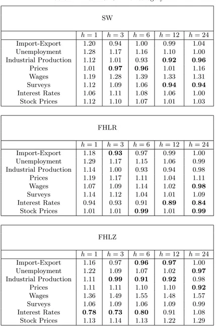
As in [11], this exercise has been extended to the other variables in the dataset. In table 4, we report the mean RMSFEs of each class of real (the first three) and nominal (the others) time series, taking AR as a benchmark. Similar results are obtained for the median and not reported here. The best performances are given in bold. We have excluded the categories “Demand”, “Money” and ”Exchange Rates’, since AR outperformed all factor models at any horizon.

AR outperforms all methods at horizon h = 1 for all cathegories, ex-cept for Interest Rates. Also, AR generally outperforms the dynamic factor models at shorter horizons (within 6 months) and it is the best methods also at h = 12 for Unemployment and Wages. As to the factor models, FHLZ seem to be the most accurate methods for real variables. Instead, no method seems to be sistematically the most performing in forecasting the nominal variables. In any case, dynamic methods seem to produce more precise forecasts than SW both on nominal and real variables. In table 5, the distribution of the RMSE of the dynamic models for each cathegories

(13)

2005-01-01 2010-01-01 2015-01-01 Time -10 -5 0 5 Fluctuation Test

IP SWvsAR -6-step ahead

Fluctuation Test Critical Value 2005-01-01 2010-01-01 Time -10 -5 0 5 Fluctuation Test

Fluctuation Test Critical Value 2005-01-01 2010-01-01 2015-01-01 Time -10 -5 0 5 Fluctuation Test

IP FHLRvsAR -6-step ahead

Fluctuation Test Critical Value 2005-01-01 2010-01-01 Time -15 -10 -5 0 5 Fluctuation Test

IP FHLZvsAR -6-step ahead

Fluctuation Test Critical Value 2005-01-01 2010-01-01 2015-01-01 Time -15 -10 -5 0 5 10 15 Fluctuation Test IP FHLRvsSW -6-step ahead Fluctuation Test Critical Value 2005-01-01 2010-01-01 Time -5 0 5 10 15 20 Fluctuation Test IP FHLRvsSW -12-step ahead Fluctuation Test Critical Value 2005-01-01 2010-01-01 Time -5 0 5 10 15 Fluctuation Test IP FHLRvsSW -24-step ahead Fluctuation Test Critical Value 2005-01-01 2010-01-01 2015-01-01 Time -20 -15 -10 -5 0 5 Fluctuation Test IP FHLZvsSW -6-step ahead Fluctuation Test Critical Value 2005-01-01 2010-01-01 Time -5 0 5 10 15 20 Fluctuation Test IP FHLZvsSW -12-step ahead Fluctuation Test Critical Value 2005-01-01 2010-01-01 Time -5 0 5 10 15 Fluctuation Test IP FHLZvsSW -24-step ahead Fluctuation Test Critical Value 2005-01-01 2010-01-01 2015-01-01 Time -15 -10 -5 0 5 10 Fluctuation Test IP FHLZvsFHLR -6-step ahead Fluctuation Test Critical Value 2005-01-01 2010-01-01 Time -20 -15 -10 -5 0 5 Fluctuation Test IP FHLZvsFHLR -12-step ahead Fluctuation Test Critical Value 2005-01-01 2010-01-01 Time -5 0 5 10 15 20 Fluctuation Test IP FHLZvsFHLR -24-step ahead Fluctuation Test Critical Value

(14)

2005-01-01 2010-01-01 2015-01-01 Time -15 -10 -5 0 5 Fluctuation Test

CPI SWvsAR -6-step ahead

Fluctuation Test Critical Value 2005-01-01 2010-01-01 Time -5 0 5 10 Fluctuation Test

CPI FHLRvsAR -6-step ahead

Fluctuation Test Critical Value 2005-01-01 2010-01-01 Time -5 0 5 10 15 Fluctuation Test

Fluctuation Test Critical Value 2005-01-01 2010-01-01 2015-01-01 Time -5 0 5 Fluctuation Test

CPI FHLZvsAR -6-step ahead

Fluctuation Test Critical Value 2005-01-01 2010-01-01 2015-01-01 Time -15 -10 -5 0 5 Fluctuation Test

CPI FHLRvsSW -6-step ahead

CPI FHLZvsSW -6-step ahead

CPI FHLZvsFHLR -6-step ahead

Fluctuation Test Critical Value

(15)

Table 4. Mean RMSFE for category. SW h = 1 h = 3 h = 6 h = 12 h = 24 Import-Export 1.20 0.94 1.00 0.99 1.04 Unemployment 1.28 1.17 1.16 1.10 1.00 Industrial Production 1.12 1.01 0.93 0.92 0.96 Prices 1.01 0.97 0.96 1.01 1.16 Wages 1.19 1.28 1.39 1.33 1.31 Surveys 1.12 1.09 1.06 0.94 0.94 Interest Rates 1.06 1.11 1.08 1.06 1.00 Stock Prices 1.12 1.10 1.07 1.01 1.03 FHLR h = 1 h = 3 h = 6 h = 12 h = 24 Import-Export 1.18 0.93 0.97 0.99 1.00 Unemployment 1.29 1.17 1.15 1.06 0.99 Industrial Production 1.14 1.00 0.93 0.94 0.98 Prices 1.19 1.17 1.11 1.04 1.11 Wages 1.07 1.09 1.14 1.02 0.98 Surveys 1.14 1.12 1.04 1.01 1.09 Interest Rates 0.94 0.93 0.91 0.89 0.84 Stock Prices 1.01 1.01 0.99 1.01 0.99 FHLZ h = 1 h = 3 h = 6 h = 12 h = 24 Import-Export 1.16 0.97 0.96 0.97 1.00 Unemployment 1.22 1.09 1.07 1.02 0.97 Industrial Production 1.11 0.99 0.91 0.92 0.98 Prices 1.11 1.11 1.10 1.10 0.92 Wages 1.36 1.49 1.55 1.48 1.57 Surveys 1.06 1.09 1.06 1.09 0.99 Interest Rates 0.78 0.73 0.80 0.91 1.08 Stock Prices 1.13 1.14 1.13 1.22 1.29

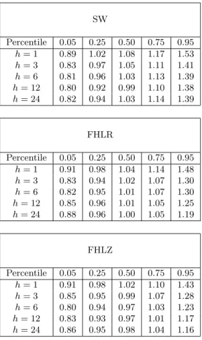
are reported. The configuration of the parameters is the one chosen in the calibration process for the forecasting of the IP. Similar results are obtained for the configurations adopted for the CPI and are not reported here.

FHLZ is the only method which improves for at least half of the series More precisely, FHLZ is as accurate as AR till half of the series at horizon h = 1. At the other horizons, it is as accurate as AR till the 75-th percentile. SW is outperformed by frequency domain methods at all horizons and at

(16)

Table 5. Distribution of the RMSFE. SW Percentile 0.05 0.25 0.50 0.75 0.95 h = 1 0.89 1.02 1.08 1.17 1.53 h = 3 0.83 0.97 1.05 1.11 1.41 h = 6 0.81 0.96 1.03 1.13 1.39 h = 12 0.80 0.92 0.99 1.10 1.38 h = 24 0.82 0.94 1.03 1.14 1.39 FHLR Percentile 0.05 0.25 0.50 0.75 0.95 h = 1 0.91 0.98 1.04 1.14 1.48 h = 3 0.83 0.94 1.02 1.07 1.30 h = 6 0.82 0.95 1.01 1.07 1.30 h = 12 0.85 0.96 1.01 1.05 1.25 h = 24 0.88 0.96 1.00 1.05 1.19 FHLZ Percentile 0.05 0.25 0.50 0.75 0.95 h = 1 0.91 0.98 1.02 1.10 1.43 h = 3 0.85 0.95 0.99 1.07 1.28 h = 6 0.80 0.94 0.97 1.03 1.23 h = 12 0.83 0.93 0.97 1.01 1.17 h = 24 0.86 0.95 0.98 1.04 1.16

almost all percentiles. Within frequency domain methods, FHLZ performs the best at 5-th and 95-th percentile.

6. Conclusions

In this paper, the forecasting performances of SW, FHLR and FHLZ are compared on a EU macroeconomic dataset which spans from February 1986 to November 2015. The EU dataset is split into two parts: the former is called calibration set and is used to tune the parameters of the dynamic factor models. The latter is called proper sample and is used to compare the forecasting performances of the three dynamic factor models. In the proper sample, all methods outperform AR after the first crisis at horizons h 6= 24. Instead, at horizon h = 24, all methods tend to lose ground against AR after the first crisis. Moreover, FHLZ generally outperforms all methods on the prediction of the CPI. Instead, no method seems to outperform in

(17)

forecasting the IP, but all dynamic factor models outperform the bench-mark AR. In the forecasting the whole dataset exercise, FHLZ is the most performing method in predicting real variables, whereas no significant evi-dencies appear on the prediction of nominal variables. However, apart from Interest Rates, all methods seem to perform poorly in comparison with AR.

Acknowledgements

We would like to thank Donatella Albano, Alessandro Giovannelli, Fab-rizio Laurini, Marco Lippi, Simona Sanfelici, Stefano Soccorsi and an anon-imous referee for their support and comments on an earlier version of the manuscript.

Appendix: Dataset and transformation

In table A.1, the series which compose the dataset are reported. T code identifies the tranformation (further details are given below) and Des iden-tifies the deseasonalized flag (1 if the series is deseasonalized, 0 otherwise). The Transformation Codes, Tcode, in table A.1, are defined as reported below: (16) zit= xitδ(Tcode− 1) + [(1 − L)xit]δ(Tcode− 2) +[(1 − L)2xit]δ(Tcode− 3) + ln (xit)(Tcode− 4) +(1 − L) ln (xit)δ(Tcode− 5) + (1 − L)2ln (xit)δ(Tcode− 6) +(1 − L)(1 − L12) ln (xit)δ(Tcode− 7),

where xit represents the raw time series xi at time t and δ(.) the Dirac

(18)

F

abio

Della

Marr

a

1 BDM1....A BD MONEY SUPPLY - M1 - CURA 6 1

2 BDM2C...B BD MONEY SUPPLY - M2 CURA 6 0

3 BDM3C...B MONEY SUPPLY - M3 - CURA 6 0

4 FRM1....A FR MONEY SUPPLY - M1 - CURN 6 1

7 ITM1....A IT MONEY SUPPLY: M1 - CURN 6 1

8 ITM2....A IT MONEY SUPPLY: M2 - CURN 6 1

9 ITM3....A MONEY SUPPLY: M3 - CURN 6 1

10 NLM1....A NL MONEY SUPPLY - M1 - CURN 6 1

13 EMECBM1.B EM MONEY SUPPLY: M1 - CURA 6 0

14 EMM2....B EM MONEY SUPPLY: M2 - CURA 6 0

15 EMECBM3.B EM MONEY SUPPLY: M3 - CURA 6 0

16 NLIMPGDSA NL IMPORTS - CIF - CURN 5 1

17 NLEXPGDSA NL EXPORTS - FOB - CURN 5 1

18 FRIMPGDSB FR IMPORTS FOB - CURA 5 1

19 FREXPGDSB FR EXPORTS FOB - CURA 5 1

20 ESOXT003b ES ITS EXPORTS F.O.B. TOTAL - CURA 5 1

21 ESOXT009b ES ITS IMPORTS C.I.F. TOTAL - CURA 5 1

22 ESEXPGDSD ES EXPORTS - CONA 5 1

23 ESIMPGDSD ES IMPORTS - CONA 5 1

24 ESEXPPRCF ES EXPORT UNIT VALUE INDEX - NADJ 5 1

25 ESIMPPRCF ES IMPORT UNIT VALUE INDEX - NADJ 5 1

26 BDEXPGDSB BD EXPORTS OF GOODS (FOB) - CURA 5 1

27 BDIMPGDSB BD IMPORTS OF GOODS (CIF) - CURA 5 1

28 BDEXPPRCF BD EXPORT PRICE INDEX - NADJ 7 1

29 BDIMPPRCF BD IMPORT PRICE INDEX - NADJ 7 1

30 ITEXPPRCF IT EXPORT UNIT VALUE INDEX - NADJ 7 1

31 BDOCC011 BD REAL EFFECTIVE EXCHANGE RATES - CPI BASED - NADJ 5 0

32 BGOCC011 BG REAL EFFECTIVE EXCHANGE RATES - CPI BASED - NADJ 5 0

33 ESOCC011 ES REAL EFFECTIVE EXCHANGE RATES - CPI BASED - NADJ 5 0

34 FNOCC011 FN REAL EFFECTIVE EXCHANGE RATES - CPI BASED - NADJ 5 0

60

Authenticated | Fabio.dellamarra@iispascal.it

(19)

orecasting perf or mance compar ison of dynamic factor models

38 ITOCC011 IT REAL EFFECTIVE EXCHANGE RATES - CPI BASED - NADJ 5 0

39 NLOCC011 NL REAL EFFECTIVE EXCHANGE RATES - CPI BASED - NADJ 5 0

40 OEOCC011 OE REAL EFFECTIVE EXCHANGE RATES - CPI BASED - NADJ 5 0

41 PTOCC011 PT REAL EFFECTIVE EXCHANGE RATES - CPI BASED - NADJ 5 0

42 BDESPPINF BD PPI: MIG - NON-DURABLE CONSUMER GOODS - NADJ 7 0

43 BDPROPRCF BD PPI: INDL. PRODUCTS, TOTAL, SOLD ON THE DOMESTIC MARKET -NADJ 7 0

44 BDESPPIEF BD PPI: MIG - ENERGY - NADJ 7 0

45 FRESPPITF FR PPI: MIG - INTERMEDIATE GOODS - NADJ 7 0

46 ITESPPINF IT PPI: MIG - NON-DURABLE CONSUMER GOODS -NADJ 7 0

47 ITESPPIEF IT PPI: MIG - ENERGY - NADJ 7 0

48 ESESPPITF ES PPI: MIG - INTERMEDIATE GOODS - NADJ 7 0

49 ESESPPINF ES PPI: MIG - NON-DURABLE CONSUMER GOODS - NADJ 7 0

50 ESPPDCNSF ES PPI - CONSUMER GOODS, DURABLES - NADJ 7 0

51 ESPPINVSF ES PPI - CAPITAL GOODS - NADJ 7 0

52 ESESPPIEF ES PPI: MIG - ENERGY - NADJ 7 0

53 ESPROPRCF ES PPI -NADJ 7 1

54 BGESPPITF BG PPI: MIG - INTERMEDIATE GOODS - NADJ 7 0

55 BGESPPINF BG PPI: MIG - NON-DURABLE CONSUMER GOODS - NADJ 7 1

56 BGESPPIIF BG PPI: INDUSTRY - NADJ 7 0

57 NLESPPITF NL PPI: MIG - INTERMEDIATE GOODS - NADJ 7 0

58 EKPROPRCF EK PPI: INDUSTRY - NADJ 7 0

59 ITCPWORKF IT CPI EXCLUDING TOBACCO (FOI) - NADJ 7 0

60 ITCP7500F IT CPI (1975=100) - NADJ 7 0

61 ITRAWPRCF IT RAW MATERIALS PRICE INDEX - NADJ 7 0

62 ITPROPRCF IT PPI - NADJ 7 0

63 FRCONPRAF FR CPI (LINKED & REBASED) - NADJ 7 0

64 FRAGPRC.F FR AGRICULTURAL PRICE INDEX - NADJ 7 0

65 FRAGIIGSF FR AGRICULTURAL INPUT PRICES - INVESTMENT GOODS & SERVICES - NADJ 7 1

66 BDCP7500F BD CPI (1975=100) - NADJ 7 1

67 ESCONPRCF ES CPI - NADJ 7 0

68 NLCONPRCF NL CPI - NADJ 7 0

69 EMCONPRCF EM CPI - NADJ 7 0

70 BDI..RELF BD REAL EFFECTIVE FX RATE (REER) BASED ON UNIT LABOUR COSTS - NADJ 5 0

61

(20)

F

abio

Della

Marr

a

74 FRI..RELF FR REAL EFFECTIVE FX RATE (REER) BASED ON UNIT LABOUR COSTS - NADJ 5 0

75 ITI..RELF IT REAL EFFECTIVE FX RATE (REER) BASED ON UNIT LABOUR COSTS - NADJ 5 1

76 ITWAGES.F IT CONTRACTUAL HOURLY WAGE: ALL WORKERS - NADJ 5 1

77 ITOLC007H IT HOURLY WAGE RATE: INDUSTRY INCL. CONSTRUCTION - PROXY NADJ 5 1

78 ITWAGES%F IT CONTRACTUAL HOURLY WAGE: ALL WORKERS (%YOY) - NADJ 5 0

79 NLI..RELF NL REAL EFFECTIVE FX RATE (REER) BASED ON UNIT LABOUR COSTS - NADJ 5 0

80 NLOLC007H NL HOURLY WAGE RATE: MFG - PROXY NADJ 5 1

81 BDIPTOT.G BD INDUSTRIAL PRODUCTION INCLUDING CONSTRUCTION (CAL ADJ) - VOLA 5 0

82 BDESPISDH BD IPI: MIG - DURABLE CONSUMER GOODS, VOLUME IOP (WDA) - VOLN 5 1

83 BDESPIESH BD IPI: MIG-CAPITAL GOODS, VOLUME INDEX OF PRODUCTION (WDA) - VOLN 5 1

84 BDESPISNH BD IPI: MIG - NON-DURABLE CONSUMER GOODS, VOLUME IOP (WDA) - VOLN 5 1

85 ESIPINTGH ES INDUSTRIAL PRODUCTION - INTERMEDIATE GOODS - VOLN 5 1

86 ESIPINVSH ES INDUSTRIAL PRODUCTION - CAPITAL GOODS - VOLN 5 1

87 ESESIBASG ES IPI: MANUFACTURE OF BASIC METALS, VOLUME IOP (WDA) - VOLA 5 0

88 ESIPOMNPH ES INDUSTRIAL PRODUCTION OTHER NONMETAL MINERAL PRODUCTS

-VOLN 5 1

89 ESIPTOT.G ES INDUSTRIAL PRODUCTION (WDA) - VOLA 5 0

90 ITIPTOT.G IT INDUSTRIAL PRODUCTION - VOLA 5 0

91 NLIPTOT.G NL INDUSTRIAL PRODUCTION EXCLUDING CONSTRUCTION - VOLA 5 0

92 FRIPTOT.G FR INDUSTRIAL PRODUCTION - VOLA 5 0

93 EU18 EK PRODUCTION - TOTAL INDUSTRY EXCL. CONSTRUCTION - VOLA 5 0

94 BDNEWORDE BD MANUFACTURING ORDERS - SADJ 5 0

95 BDRVNCARP BD NEW PASSENGER CAR REGISTRATIONS - VOLN 5 1

96 BGACECARP BG NEW PASSENGER CAR REGISTRATIONS - VOLN 5 1

97 ESCAR...O ES REGISTRATIONS: PASSENGER CAR - VOLA 5 0

98 FRCARREGO FR NEW CAR REGISTRATIONS (CAL ADJ) -VOLA 5 0

99 FRHCONMFD FR HOUSEHOLD CONSUMPTION - MANUFACTURED GOODS - CONA 5 0

100 FRHCONDGD FR HOUSEHOLD CONSUMPTION - DURABLE GOODS - CONA 5 0

101 ITNEWORDF IT NEW ORDERS - NADJ 5 1

102 ITRETTOTF IT RETAIL SALES - NADJ 5 1

103 BDCNFCONQ BD CONSUMER CONFIDENCE INDICATOR - GERMANY - SADJ 2 0

104 BGCNFCONQ BG BNB CONS. SVY.: CONSUMER CONFIDENCE INDICATOR (EP) - SADJ 2 0

105 BGCNFBUSQ BG BUSINESS INDICATOR SURVEY - ECONOMY - SADJ 2 0

106 BGEUSIOBQ BG IND.: OVERALL - ORD BOOKS - SADJ 2 0

62

(21)

orecasting perf or mance compar ison of dynamic factor models

110 BGSURECSQ BG BNB CONS.SVY.: ECON.SITUATION- FCST. OVER NEXT 12 MONTHS - SADJ 2 0

111 BGSURPUHQ BG BNB CONS.SVY.: MAJOR HH.PURCH-FCST.OVER NEXT 12 MONTHS(EP) 2 0

112 ESINT384R ES PRODUCTION LEVEL - INDUSTRY - NADJ 2 0

113 FRINDSYNQ FR SURVEY: MANUFACTURING - SYNTHETIC BUSINESS INDICATOR - SADJ 2 0

114 FRSURPMPQ FR SURVEY: MANUFACTURING OUTPUT - RECENT OUTPUT TREND - SADJ 2 0

115 FRSURGMPQ FR SURVEY: MANUFACTURING OUTPUT - ORDER BOOK & DEMAND - SADJ 2 0

116 FRSURGPDQ FR SURVEY: MANUFACTURING OUTPUT LEVEL - GENERAL OUTLOOK - SADJ 2 0

117 FRSURTMPQ FR SURVEY: MANUFACTURING OUTPUT - PERSONAL OUTLOOK - SADJ 2 0

118 ITHHFECSR IT HOUSEHOLD CONFIDENCE SURVEY: FUTURE FINANCIAL POSITION - NADJ 2 0

119 ITCNFCONQ IT HOUSEHOLD CONFIDENCE INDEX - SADJ 5 0

120 NLCNFBUSQ NL CBS MFG. SVY.: PRODUCER CONFIDENCE INDEX - SADJ 2 0

121 NLEUSCPCR NL CONSUMER SURVEY: MAJOR PURCH.OVER NEXT 12

MONTHS-NETHERLANDS 2 0

122 EKCNFBUSQ EK INDUSTRIAL CONFIDENCE INDICATOR - EA - SADJ 2 0

123 EMEUSCCIQ EM CONSUMER CONFIDENCE INDICATOR - EA - SADJ 2 0

124 EKEUSIPAQ EK INDUSTRY SURVEY: PRODUCTION EXPECTATIONS (EA) - SADJ 2 0

125 EKEUBCI.R EK BUSINESS CLIMATE INDICATOR-COMMON FACTOR IN IND. (EA) - NADJ 2 0

126 EKEUSESIG EK ECONOMIC SENTIMENT INDICATOR (EA18) - VOLA 5 0

127 EMGBOND. EM GOVERNMENT BOND YIELD - 10 YEAR 2 0

128 EMECB2Y. EM GOVERNMENT BOND YIELD - 2 YEAR 2 0

132 BDESSFUB BD HARMONISED GOVERNMENT 10-YEAR BOND YIELD 2 0

133 FRESSFUB FR HARMONISED GOVERNMENT 10-YEAR BOND YIELD 2 0

134 ESESSFUB ES HARMONISED GOVERNMENT 10-YEAR BOND YIELD 2 0

135 BGESSFUB BG HARMONISED GOVERNMENT 10-YEAR BOND YIELD 2 0

136 ITESSFUB IT HARMONISED GOVERNMENT 10-YEAR BOND YIELD 2 0

137 ITINTER3 IT INTERBANK DEPOSIT RATE-AVERAGE ON 3-MONTHS DEPOSITS 2 0

138 MSEROP$ E MSCI EUROPE U$ - PRICE INDEX 5 0

139 INDGSIT& E ITALY-DS Inds Gds & Svs - PRICE INDEX 5 0

140 INDGSBD& E GERMANY-DS Inds Gds & Svs - PRICE INDEX 5 0

141 INDGSFR& E FRANCE-DS Inds Gds & Svs - PRICE INDEX 5 0

142 INDUSBD E GERMANY-DS Industrials - PRICE INDEX 5 0

63

(22)

F

abio

Della

Marr

a

146 FINANBD E GERMANY-DS Financials - PRICE INDEX 5 0

147 FINANIT E ITALY-DS Financials - PRICE INDEX 5 0

148 CNSMGFR E FRANCE-DS Consumer Gds - PRICE INDEX 5 0

149 CNSMGBD E GERMANY-DS Consumer Gds - PRICE INDEX 5 0

150 CNSMGIT E ITALY-DS Consumer Gds - PRICE INDEX 5 0

151 OILGSEM E EMU-DS Oil & Gas - PRICE INDEX 5 0

152 BMATREM E EMU-DS Basic Mats - PRICE INDEX 5 0

153 INDUSEM E EMU-DS Industrials - PRICE INDEX 5 0

154 RITDVEM E EMU-DS Divers. REITs - PRICE INDEX 5 0

155 CNSMGEM E EMU-DS Consumer Gds - PRICE INDEX 5 0

156 HLTHCEM E EMU-DS Health Care - PRICE INDEX 5 0

157 TELCMEM E EMU-DS Telecom - PRICE INDEX 5 0

158 UTILSEM E EMU-DS Utilities - PRICE INDEX 5 0

159 FINANEM E EMU-DS Financials - PRICE INDEX 5 0

160 CNSMSEM E EMU-DS Consumer Svs - PRICE INDEX 5 0

161 TECNOEM E EMU-DS Technology - PRICE INDEX 5 0

162 EMSHRPRCF EM DATASTREAM EURO SHARE PRICE INDEX (MONTHLY AVERAGE) - NADJ 5 0

163 BDMLM006Q BD REGISTERED UNEMPLOYMENT: RATE (ALL PERSONS) - SADJ 2 0

164 BDMLM005O BD REGISTERED UNEMPLOYMENT: LEVEL (ALL PERSONS) - VOLA 5 0

165 ITMLFT15O IT HARMONISED UNEMPLOYMENT: LEVEL, ALL PERSONS (ALL AGES) - VOLA 5 0

166 ITMLRT16Q IT HARMONISED UNEMPLOYMENT: RATE, ALL PERSONS (ALL AGES) - SADJ 2 0

167 ITMLRT14Q IT HARMONISED UNEMPLOYMENT: RATE, ALL PERSONS (AGES 15-24) - SADJ 2 0

168 ITMLRF16Q IT HARMONISED UNEMPLOYMENT: RATE, FEMMES (ALL AGES) - SADJ 2 0

169 ITMLRM16Q IT HARMONISED UNEMPLOYMENT: RATE, HOMMES (ALL AGES) - SADJ 2 0

170 FRESTUNPO FR UNEMPLOYMENT: TOTAL - TOTAL - VOLA 5 0

171 FRMLRT14Q FR HARMONISED UNEMPLOYMENT: RATE, ALL PERSONS (AGES 15-24) - SADJ 2 0

172 FRMLRT15Q FR HARMONISED UNEMPLMT.: RATE,ALL PERSONS(AGES 25 AND OVER)

-SADJ

2 0

173 FRMLRT16Q FR HARMONISED UNEMPLOYMENT: RATE, ALL PERSONS (ALL AGES) -SADJ 2 0

174 FRMLRF16Q FR HARMONISED UNEMPLOYMENT: RATE, FEMMES (ALL AGES) - SADJ 2 0

175 FRMLRm16Q FR HARMONISED UNEMPLOYMENT: RATE, HOMMES (ALL AGES) - SADJ 2 0

176 ESMLM005O ES HARMONISED UNEMPLOYMENT: LEVEL, ALL PERSONS (ALL AGES) - VOLA 5 0

64

(23)

REFERENCES

1. J. H. Stock and M. W. Watson, Forecasting using principal components from a large number of predictors, Journal of the American Statistical Association, vol. 97, no. 460, pp. 1167–1179, 2002a.

2. J. H. Stock and M. W. Watson, Macroeconomic forecasting using diffu-sion indexes, Journal of Business & Economic Statistics, vol. 20, no. 2, pp. 147–162, 2002b.

3. M. Forni, M. Hallin, M. Lippi, and L. Reichlin, The generalized dynamic factor model: Identification and estimation, Review of Economics and Statistics, vol. 82, no. 4, pp. 540 – 554, 2000.

4. M. Forni, M. Hallin, M. Lippi, and L. Reichlin, The generalized dy-namic factor model: One-sided estimation and forecasting, Journal of the American Statistical Association, vol. 100, pp. 830 – 840, 2005. 5. M. Forni, M. Hallin, M. Lippi, and P. Zaffaroni, Dynamic factor model

with infinite dimensional factor space: representation, Journal of Econo-metrics, vol. 185, pp. 359–371, 2015.

6. M. Forni, M. Hallin, M. Lippi, and P. Zaffaroni, Dynamic factor model with infinite dimensional factor space: Asymptotic analysis, tech. rep., EIEF Working Paper 2016/07, Einaudi Institute for Economics and Finance, 2016.

7. J. Boivin and S. Ng, Understanding and comparing factor-based fore-casts, International Journal of Central Banking, vol. 1, no. 3, pp. 117 – 151, 2005.

8. A. D’ Agostino and D. Giannone, Comparing alternative predictors based on large-panel factor models, Oxford bulletin of economics and statistics, vol. 74, no. 2, pp. 306–326, 2012.

9. C. Schumacher, Forecasting german gdp using alternative factor models based on large datasets, Journal of Forecasting, vol. 26, no. 4, pp. 271– 302, 2007.

10. A. H. den Reijer et al., Forecasting dutch gdp using large scale factor models, tech. rep., Netherlands Central Bank, Research Department, 2005.

11. M. Forni, A. Giovannelli, M. Lippi, and S. Soccorsi, Dynamic factor model with infinite dimensional factor space: forecasting, tech. rep.,

(24)

CEPR Discussion Paper No. DP11161, 2016.

12. M. Forni and M. Lippi, The generalized dynamic factor model: repre-sentation theory, Econometric theory, vol. 17, no. 06, pp. 1113–1141, 2001.

13. M. Hallin and M. Lippi, Factor models in high-dimensional time series: A time-domain approach, Stochastic Processes and their Applications, vol. 123, no. 7, pp. 2678–2695, 2013.

14. M. Forni, D. Giannone, M. Lippi, and L. Reichlin, Opening the black box: Structural factor models with large cross sections, Econometric Theory, vol. 25, no. 05, pp. 1319–1347, 2009.

15. R. Giacomini and H. White, Tests of conditional predictive ability, Econometrica, vol. 74, no. 6, pp. 1545–1578, 2006.

16. R. Giacomini and B. Rossi, Forecast comparisons in unstable environ-ments, Journal of Applied Econometrics, vol. 25, no. 4, pp. 595–620, 2010.