Università degli Studi di Salerno
DIPARTIMENTO DI SCIENZE ECONOMICHE E STATISTICHE
Davide Cantarelli
Department of Economics - University of Padova [email protected]
E
LASTICITIES OFC
OMPLEMENTARITY ANDS
UB-STITUTION IN
S
OMEF
UNCTIONALF
ORMS.
A
C
OMPARATIVER
EVIEW*
WORKING PAPER 3.157 febbraio 2005
* Thanks are due to Piero Tani, Giandemetrio Marangoni and Sergio Destefanis for some useful suggestions, and to Dr. Licia Salce for her help in calculations
Index
1. Introduction ... 7
2. Functional Forms ... 9
3. Inflexible Functional Forms... 14
4. Flexible Functional Forms: a) Diewert’s GL and Translog... 21
5. Flexible Functional Forms: b) Lau’s Quadratic and Diewert’s Generalized Cobb-Douglas, Extended by Magnus ... 29
6. Final Considerations... 34
Appendix ... 38
Abstract
This paper presents and discusses the results of a comparative review of the elasticities of complementarity and substitution which may be obtained from seven functional forms, inflexible and flexi-ble. Every functional form is examined in its four versions: produc-tion, cost, profit, and distance. The elasticities of complementarity were obtained from the production and distance functions (elastic-ities of Hicks, Antonelli and Morishima), and those of substitution from the cost and profit functions (elasticities of Allen-Uzawa and Lau). The results of the calculations of the various elasticities are compared and evaluated.
JEL Classification:
D21, D24
1. Introduction
Many, reading the title of this paper, will object that there is no need for such a survey. The main task of this introduction is there-fore to justify this work.
The contemporary substitutability and complementarity of pro-duction factors is certainly one of the most important grounds of theoretical and applied research on the phenomena of production and distribution. To the initial analytical instrument, i.e., the produc-tion funcproduc-tion, thanks to the development of the duality theory, func-tions of cost, profit and distance have been added, and applied to numerous functional forms with equally numerous “variants” and extensions, mainly put forward in the twenty-year period 1970-1990. It is well-known that the main reason for proposing flexible functional forms (FFF) was the wish (and also, objectively, the need) to use them to increase the possibility of variation of the elasticity of substitution among the factors (i.e., what was defined – in our view, improperly – as a “second-order parameter”) with re-spect to the elasticity permitted by inflexible functional forms (IFF). Theoretical contributions and relative discussions on the elasticity
sion from a production function with two factors to one with n fac-tors2. A very different fate was that of the elasticity of complemen-tarity, which has received far less attention - even less than that justified by its more specific and limited field of application3. After the work by J.R. Hicks (1970), in which the author credited Joan Robinson with having created the elasticity of substitution while Hicks maintained that of complementarity, there were remarkably few – in absolute and not only relative terms – theoretical and ap-plicative contributions devoted to the elasticity of complementarity until the end of the last century (and millennium), when interest was renewed4. Together with this, three more facts characterise the current situation of the theory of production: first, the growing use of the distance function, which allows us to treat cases in which there is more than one output; second, the current cessation of new proposed functional forms; and third, the development and spread of the “non-parametric” analysis of production.
This set of conditions suggested the idea of surveying a cer-tain number of functional forms in their quadruple aspects of pro-duction, cost, profit, and distance, and the elasticities of substitu-tion and complementarity deriving from them. By highlighting par-ticular aspects which may escape a superficial examination, we hope to make the survey more interesting – not just a manual or a “reference paper” for the future. We do not consider here the as-pects and problems of the econometric application of the functional forms examined here, since they are beyond both the author’s ca-pacity and competence and the proper dimensions of a paper.
This work has six sections. Section 2 presents the functional forms examined here, their layout, and the list of uniform symbols which are used. Section 3 presents and discusses IFF formulas, and sections 4 and 5 FFF formulas. Section 6 makes conclusive considerations.
2
See Blackorby and Russel (1989).
3
It has been rightly noted (Kim, 2000) that the elasticity of complementarity is useful when there are constraints to the quantities of inputs, so that their prices are distorted or even non-existent. It measures the substitutability of inputs in terms of their quantities.
4
From 1970 to 1991, only about a dozen theoretical and applicative contributions to Hicks’ elasticity of complementarity appeared in leading journals, i.e., a number not comparable with contributions regarding the elasticity of substitution. See Kim (2000) for references.
2. Functional Forms
The functional forms examined in this survey are three IFF, i.e., Cobb-Douglas (CD), CES-ACMS (Arrow, Chenery, Minhas, Solow 1961) and CMC-CES5, and four FFF, i.e., Translog, Diew-ert’s Generalized Leontiev (DGL 1971), Lau’s Quadratic (LQ 1978), and Diewert’s Generalized Cobb-Douglas (1973), corrected and extended by Magnus (MEDGCD) (1979). The survey opens with the Cobb-Douglas IFF, with all its constant and unitary elastic-ities, as an act of homage to and respect for a cornerstone in the construction of the theory of production and as an analytical tool which – rightly or wrongly – is still used6. The CES-ACMS has constant elasticities but they are not always equal for the four func-tions. The CMC-CES is homothetic, like the previous two, but not homogeneous, and it has properties which are partly equal and partly different. Among the FFF, there are, of course, Translog and DGL, because they are the forms mostly frequently applied with respect to the other two, Lau’s Quadratic and MEDGCD.
MEDGCD is presented in place of the original function (1973), because the latter has the defect that estimations of its primary and secondary parameters (and thus also their elasticities) are not invariant with respect to the multiplicative scaling of input prices7. Every function form is accompanied by its formulas for the func-tions of: production, cost, profit, distance, elasticity of substitution or of complementarity, demand or quota of input cost, scale economies and size economies8. It should be recalled that the
5
On the characteristics and properties of the CMC-CES function, see Cantarelli, Di Fonzo and Giacomello (1994).
6
Its use remains extended to the macro level even if it non is limited to the micro level.
7
pre-functions of the elasticity of complementarity have as their argu-ments the physical quantities of productive inputs and are thus ob-tained from the production and distance functions, whereas those of the elasticity of substitution have as their arguments costs (nor-malised, or less so, in various ways) of inputs. The elasticities of complementarity presented here are those of Hicks, Antonelli and Morishima (1967). While Hicks’ elasticity of complementarity is ob-tained from the production function, that yielded by the distance function is called “Antonelli’s elasticity” (1886), to recall both that he was the first to define the concept of inverse demand functions (Cornes (1992) and Kim (2000)), and that Antonelli’s substitution matrix is precisely the matrix of second partial derivatives of the distance function in the consumer theory (Deaton (1979) and thus of the producer. Morishima’s elasticities of complementarity, pro-posed by Kim (2000), are also derived from the distance function. The elasticities of substitution are those of Allen-Uzawa (1962) and Morishima (1967), taken from the cost functions, and that of Hotelling-Lau, taken from the profit function9. Allen’s (1938) elastic-ity of substitution, yielded by the production function with n inputs, is not examined here, because the author shares the opinion of authoritative experts that it does not give a correct measure of the
duced. The ratio xo+/ xo is the maximum scalar λ for which xo may be divided and still produce yo. In symbols, λ=DI
(
x ,yo+ o)
≡max{
λ| f x /(
o+ λ)
≥yo}
. The maximum value of λ depends on the choice of xo+ and yo, and the distance function precisely expresses this dependence. In symbols, D ( )y ,x max{
| /(1 )x, y ) possible}
I ≡ λ λ . This is the input dis-tance function, which must not be confused with the output disdis-tance function, which also exists and which mirrors it. The input distance function may easily be extended to cases of several inputs and outputs. In this case, if DI( )y,x may be differentiated twice everywhere,
( ) ( )
DI / xi wi
∂ y,x ∂ ≡ y,x is the marginal product or inverse demand function for input xi. For further details, see Cornes (1992). It is perhaps also appropriate to recall that the elas-ticity of scale measures how output varies moving along a scale line from the origin in the input space; the elasticity of size measures how cost varies along the expansion path (locus of the minimum cost) in the input space. If the production function is homothetic, the two elasticities are equivalent.
9
The name Hotelling-Lau is due to Bertoletti (2001) who refers to Chapter I.3, “Applications of Profit Functions”, of Lau’s “Production Economics”, in which Lau defines this elasticity by means of the profit function (page 197).
relation between inputs when there are more than two of them, and that this relation can be obtained with Morishima’s elasticity.
The elasticity formulas shown in the tables are mostly calcu-lated autonomously (like all the elasticities of complementarity and Morishima’s elasticity) and partly taken from authors who have proposed functional forms (e.g., the elasticities of Translog produc-tion and cost funcproduc-tions) and are all presented with uniform sym-bols. Autonomous proposals and adaptations “by analogy” have also been advanced, in cases in which one of the cost, profit or distance functions is not explicitly proposed by experts on the sub-ject10.
Given the generic function y=g( z ...z )1 n of production, cost, profit or distance, non-Morishima elasticities eij are calculated by means of the formula:
(1) 2 1 n i j ij ji i j g( z ...z ) g / z z e e ; i j ( g / z )( g / z ) ⋅∂ ∂ ∂ = = ≠ ∂ ∂ ∂ ∂
and those of Morishima by means of: (2) 2 2 2 i j i ij i i j i g / z z / z e z z g / z g / z ∂ ∂ ∂ ∂ ∂ = ⋅ − ⋅ ∂ ∂ ∂ ∂ and 2 2 2 i j j ji j j i j g / z z / z e z z g / z g / z ∂ ∂ ∂ ∂ ∂ = ⋅ − ⋅ ∂ ∂ ∂ ∂
For the FFF, the four functions are maintained in their simplest forms, i.e., uni-product, without fixed inputs, and without the addi-tion of variables in a multiplicative relaaddi-tion with the main arguments of the functions themselves, i.e., inputs or their costs, which may enter (complicating them) into the elasticity formulas through ap-posite derivatives.
used, and γ appears as an efficiency parameter. Obviously, these letters take on differing values for each of the functions to which they refer. The characteristics of the parameters are shown next to the production functions and are to be understood as extended and valid also for the other three, unless otherwise indicated. Sim-plification of the expressions resulting from the application of for-mulas (1) and (2) was carried out with varying intensity (greater for (2)), bearing in mind conditions sufficient for their easy identifica-tion.
As the number of symbols used is quite high, they are listed, for readers’ convenience, at the end of this Section and before the tables containing the functional formulas.
Symbols
y output in physical units
i
x quantity of input i
i
w nominal unit cost of input i
y
p nominal unit price of output y
i i y
q =w / p unit “normalized” cost of input i y(x) production function
C( y,w) total cost function G( )q normalized profit function D( y, )x distance function
µ scale coefficient in production function
ySi output’s share of input i in Translog production function CSi cost’s share of input i in Translog cost function
CMSi cost’s share of input i in MEDGCD cost function
( )
y,ε x elasticity of scale from production function
(
y,)
ε∗ w elasticity of size from cost function A
σ Allen’s elasticity of substitution from production function
σ constant elasticity of substitution in CES functions
(
1)
/θ = −σ σ
HEC ij
ρ Hicks’ elasticity of complementarity from production function
AEC ij
ρ Antonelli’s elasticity of complementarity from distance function
MEC MEC
ij ji
ρ ≠ρ Morishima’s elasticities of complementarity from distance function
AUES ij
σ Allen-Uzawa’s elasticity of substitution from cost function
MES MES
ij ji
σ ≠σ Morishima’s elasticities of substitution from cost function
HLES ij
3. Inflexible Functional Forms
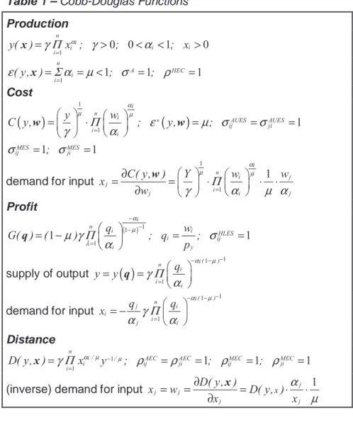
As already noted in section 2, Table 1 (Cobb-Douglas) does not require much comment. All the elasticities, including σA are positive, constant, and equal to 1. The inputs are thus always and only q-complement and p-substitutes. The total passus coefficient
( y,x )
ε =µ is assumed to be <1, in order to write the profit func-tion, which would otherwise be annulled, as the formula clearly shows. The demand functions of inputs – like all the functional forms considered here – are taken from the cost function accord-ing to Shephard’s lemma, and from the profit function accordaccord-ing to Hotelling’s lemma. The two functions are different because the one obtained from the cost function is conditional or “compensated” by the constancy of output, while that obtained from the profit function is not. Therefore, AUES
ij
σ expresses net p-substitutability and HLES ij σ gross p-substitutability.
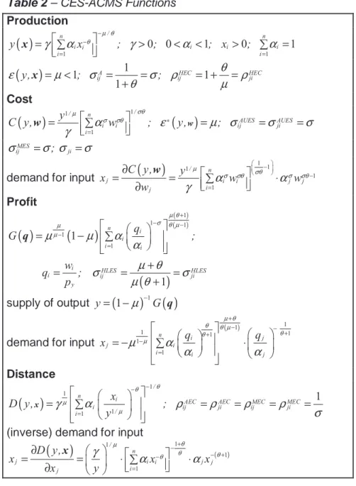
Table 2, showing the CES-ACMS functions, presents a slightly more varied situation. Production is written in the way Arrow, Chenery, Minhas and Solow wrote it in their original work of 1961, i.e., with negative exponents inside or outside square brackets11.
Also in this case, and for the same reason as for the Cobb-Douglas function, µ is assumed to be <1. One first aspect to be noted is that, although coefficient µ enters into the calculation of
HEC ij
ρ , it does not in A ij
σ . However, if µ is assumed to be equal to 1, then HEC
ij
ρ is the reciprocal of σA. In this regard, the hypothesis may be advanced that, whereas in the Cobb-Douglas function (and, as we shall see later, also in the CMC-CES) the value of µ is, as it were, “incorporated” in the function (see Table 1), and ob-tainable from it, in CES-ACMS it is a constant introduced from the outside.
11
In the same pages of “Production Economics” (see previous note), the CES function is written with positive exponents and without the γ constant. Simulations reveal that the ver-sion with negative exponents supplies values for output y which are systematically lower and in (modest) constant proportion with respect to those obtained with positive exponents. The difference in sign of the exponents of the production function affects those of the profit function.
Table 1 – Cobb-Douglas Functions Production 1 0 0 1 0 n i i i i i y( ) γ Π x ;α γ ; α ; x = = > < < > x 1 1 1 1 n A HEC i i ( y, ) ; ; ε Σ α µ σ ρ = = = < = = x Cost
(
)
(
)
1 1 1 1 1 i n i AUES AUES ij ji i i MES MES ij ji y w C y, ; y, ; ; α µ µ Π ε µ σ σ γ α σ σ ∗ = = ⋅ = = = = = w wdemand for input
1 1 1 i n i j j i j i j C( y, ) Y w w x w α µ µ Π γ = α µ α ∂ = = ⋅ ⋅ ⋅ ∂ w Profit ( )1 1 1 1 1 i n i i HLES i ij i y q w G( ) ( ) ; q ; p α µ λ µ γ Π σ α − − − = = − = = q supply of output
( )
1 1 1 ( ) i n i i i q y y α µ γ Π α − − − = = = qdemand for input
1 1 1 ( ) i n j i i i j i q q x α µ γ Π α α − − − = = − Distance 1 1 1 1 1 n /
i / AEC AEC MEC MEC
i ij ji ij ji i D( y, ) γ Π xα µy− µ; ρ ρ ; ρ ; ρ = = = = = = x
(inverse) demand for input j j j 1
j j x D( y, ) x w D( y, ) x x α µ ∂ = = = ⋅ ⋅ ∂ x
Table 2 – CES-ACMS Functions Production
( )
1 1 0 0 1 0 1 / n n i i i i i i i y x ; ; ; x ; µ θ θ γ α − − γ α α = = = ∑ > < < > ∑ = x( )
1 1 1 1 HEC HEC A ij ij ji y, ; ; θ ε µ σ σ ρ ρ θ µ = < = = = + = + x Cost(
)
1 1( )
1 / / n AUES AUES i i ij ji i y C y, w ; y, ; σθ µ σ σθ α ε µ σ σ σ γ = ∗ = ∑ = = = w w MES ij ; ji σ =σ σ =σdemand for input
(
)
1 1 1 1 1 / n j i i j j i j C y, y x w w w µ σθ σ σθ σ σθ α α γ − − = ∂ = = ∑ ⋅ ∂ w Profit
( )
(
)
( ) ( )(
)
1 1 1 1 1 1 1 n i i i i i HLES HLES i ij ji y q G ; w q ; p µ θ σ θ µ µ µ µ µ α α µ θ σ σ µ θ + − − − = = − ∑ + = = = + q supply of output y= −(
1 µ) ( )
−1G qdemand for input
( ) 1 1 1 1 1 1 1 n i j j i i i j q q x µ θ θ θ µ θ θ µ µ α α α + − − + + − = = − ∑ ⋅ Distance
( )
1 1 1 1 1 / n iAEC AEC MEC MEC
ij ji ij ji i / i x D y, ; y θ θ µ µ γ α ρ ρ ρ ρ σ − − = = ∑ = = = = x
(inverse) demand for input
( )
( ) 1 1 1 1 / n j i i j j i j D y, x x x x y θ µ θ θ θ γ α −+ α − + − = ∂ = = ⋅∑ ⋅ ∂ xWhen this happens, it does not modify A ij
σ but enters into the calculation of HEC
ij
ρ and does not leave it. Instead, the reciprocal of A
ij
σ is ρAEC, respecting the rule that this must happen for a function
which is homogeneous and not simply homothetic. The two MEC
ij ρ are also reciprocals of A
ij
σ . The constancy of σA is also transmit-ted to AUES
ij
σ and MES
ij
σ . Instead, a constant but different value re-sults for HLES
ij
σ , in which (as in MEC
ij
ρ ), the value of µ enters. This contemporary presence matches the duality which, it is stated, ex-ists between the production and profit functions (Bertoletti, 2001), and the circumstance that ρHEC and HLES
ij
σ respectively express a
gross q-complementarity and a gross p-substitutability.
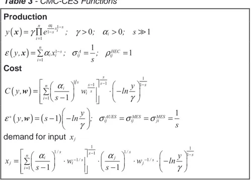
A very different situation arises with the CMC-CES functional form. Its production function is homothetic but not homogeneous,
A
σ is constant and equal to 1s, and its dual cost function is also
homothetic. Although the production function is not homogeneous, its Hicks’ elasticity of complementarity, ρHEC, is equal to 1, as in the Cobb-Douglas function – a result which was not expected a priori. The elasticities of substitution AUES
ij σ , MES ij σ and MES ji σ
obtain-able by means of the cost function, are all equal to 1 s as
ex-pected. The CMC-CES function is a special case, comparatively simpler, of the more general CMC non-homogeneous function, in which each input xi has its own si, and its elasticity σA is variable within limits defined by the relations > < =, , among the si.
Table 3 - CMC-CES Functions Production
( )
1 1 1 0 0 1 n i s xi s i i y e ; ; ; s α γ − − γ α = = ∏ > > x≫
( )
1 1 1 1 n s A HEC i i ij ij i y, x ; ; s ε α − σ ρ = =∑ = = x Cost(
)
1 1 1 1 1 1 1 s s s s s n i s i i y C y, w ln s α γ − − − = =∑ − ⋅ − w(
) (
)
11 AUES MES MES
ij ij ji y y, s ln ; s ε σ σ σ γ ∗ = − − = = = w
demand for input xj
1 1 1 1 1 1 1 1 1 1 1 / s s / s s n i / s j / s j i j i y x w w ln s s α α γ − − − − = =∑ − ⋅ ⋅ − ⋅ ⋅ −
The general CMC is a somewhat complex function, which yields the dual cost function only in very particular cases, or else by means of more or less satisfactory approximations12. Now, for such a function with a variable σA13, ρHEC is constant and equal to 1, as in the simpler Cobb-Douglas function!
Although the presence of a single s in the CMC-CES allows its dual cost function to be rendered in explicit form, this is not enough for the present writer to obtain the profit function. Lau’s procedure in the case of two preceding IFF to yield the G( )q func-tions shown in Tables 1 and 2 is – at least, in the writer’s opinion – inapplicable14, because it is based on the constancy of coefficient
12
On the approximated forms of the non-homothetic CMC cost function, see Cantarelli (1999) and (2003).
13
On σA in the CMC (not CES) function, see Cantarelli and Giacomello (1995).
14
See Lau (1978), pp. 190-192. Lau starts from the first-order condition necessary in order to have maximum profit, (∂ ∂y / xi)=w / pi y (which, for example, in the Cobb-Douglas
( )
ε x =µ (see Tables 1 and 2). In the CMC-CES, n 1s
i i i
( ) x
ε x =∑ α −
decreases variably with the increase in the quantity of inputs, passing from an initial part, in which it is >1, to the following part, in which it becomes <1. The profit and function G( )q may thus exist only starting from µ<1. Some simple simulations confirmed that
the value of µ at which maximum profit is reached is one and only one, and that it determines the maximum value of G at the same time15. In other words, µ is not only a variable but also an un-known, to be defined before or together with function G( )q , if we know how to determine it. In fact, by means of simulations it is possible to obtain the value of Gmax with every degree of approxi-mation desired, as explained in note (14), but they do not supply the equations of function G( )q and of σHLES which – at least for the moment – we must abandon.
The variability of µ also comes into play in the distance func-tion, again making it difficult to define. The CMC-CES funcfunc-tion, with an equational form only slightly more complex than that of CD and CES-ACMS, confirms the opinion of experts (cf. for example,
function) becomes (αiy / xi)=qi) and, using the mathematical procedure called “Legendre transformation”, y is substituted by its value in terms of profit function G and xi by its corresponding −∂G / q∂ i. He thus obtains for input xi a first-order differential equation with separable variables, making part of the compound system of similar equations for all n in-puts. He treats this system as an ordinary differential equation and, integrating it, obtains function G( )q . The writer dispelled his initial doubts on the legitimacy of treating the sys-tem as a single equation by means of a series of control simulations. They confirmed the result: given parameters αi and γ, and qi with constant µ and <1, functions G( )q of the Cobb-Douglas and CES-ACMS forms do give G values realizing maximum profit.
15
The simulation is effected in the following way. If there are, for instance, 3 inputs, x , x1 2 and x3, with given values of x1, the functions of the expansion paths yield the levels of x2
Cornes, 1992) regarding the difficulty of defining it outside really simple cases. For example, in the case of CMC-CES, relation
1
D( y, )x = f (x)− cannot be used (as it is later), because it is appli-cable only in the case of constant returns to scale which, as al-ready mentioned, are variable in the CMC-CES function16.
Intuition, the fact that the other elasticities of the functional form are constant, tests carried out with some “invented” functions, and the meaning of “efficient complementarity” 17 which parameter
s takes on in the production function, are all circumstances which lead us to conclude that elasticities of complementarity ρHEC and
MES
ρ must be equal to s.
However, apart from hypotheses and inferences and the real or presumed impossibility of determining the profit and distance functions of CMC-CES or any other function, it should be recalled that a way of obtaining σHLES directly from σAUES and ρHEC from
AEC
ρ and vice versa was recently proposed, not resorting to the functions themselves but to given elasticities, such as those re-garding the output of conditional or unconditional demands of in-puts and those of the total or marginal cost (Bertoletti, 2001, for-mulas 13 and 17). “Filling in” and checking these forfor-mulas by means of the above-mentioned elasticities for the functional forms
16
In this regard, see Syrquin and Hollender (1982) and Kim (2000).
17
As regards the efficient complementarity expressed by s, see Cantarelli, Di Fonzo and Giacomello (1994) and Cantarelli (1999). Out of curiosity and as proof, recourse to the equation D y,( ) ( )x =f x −1 gives ρAEC =ρHEC =1 and MES MES
ij ji s
ρ =ρ = . The result, 1
AEC HEC
ρ =ρ = , is not acceptable in the case of variable returns to scale, because HEC
ρ is an index of gross complementarity, which incorporates an output effect next to the substitution effect – contrary to what happens to the other forms, which only express the second effect (cf. note 16). Alternative versions were also tried out, which, variously, mimic the Cobb-Douglas function, exploiting the circumstance of the identity of work undertaken by exponents αi of CD and 1 s i ix α − of CMC-CES, i.e., ( ) i y,x ε =∑α and ( ) 1s i i y,x x
ε =∑α − (cf. Table 1). Mile-long expressions were obtained for ρAEC: however, possibilities of achieving further simplifications - which the computer could not or would not carry out - could not be found. Instead, for ρMEC, on similarly mile-long expressions, the computer carried out the simplifications and, for all of them, supplied s as a result, the re-ciprocal of σAUES and σMES obtained from the cost function, which is a dual of the dis-tance function.
examined here, and for others, together with a practical applica-tion, would certainly be an interesting subject for a special re-search.
4. Flexible Functional Forms: a) Diewert’s GL and Translog
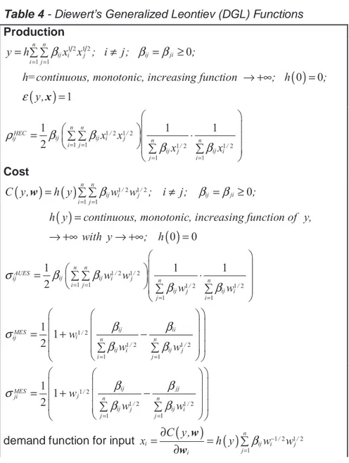
Undeniably, Diewert’s GL has the positive characteristic of simple path-breaking. It does determine linear demand functions of inputs, the econometric estimation of which is thereby facilitated, and elasticities of substitution and complementarity whose values may range over wide intervals. This appreciation is particularly and specifically true for the cost rather than for the production func-tion18. This, in our opinion, is because the former can be subjected to extensions of various types, which may transform it from homo-thetic into non-homohomo-thetic, thus making it more realistic, as econometric applications show. If we examine some extensions of it (Table 4), we can see how simple they are, easy but nonetheless significant after modification-substitution of the generic function
h( y ). Instead, as regards the production function, it is more diffi-cult to imagine what content and significance function h may take on (note the difference in writing it used by Diewert!). The quanti-ties of inputs must be excluded, because they already appear in the function. In the explicit words of the author, quoted in Table 419, h must be understood as an increasing function and not as a constant, similar to the µ which appears in the CES-ACMS, capa-ble of transforming constant returns to scale into increasing or de-creasing ones.
Table 4 - Diewert’s Generalized Leontiev (DGL) Functions Production
( )
( )
1 2 1 2 1 1 0 0 0 1 n n ij i j ij ji i j y h x x ; i j; ;h=continuous, monotonic, increasing function ; h ; y, β β β ε = = = ∑ ∑ ≠ = ≥ → +∞ = = x 1 2 1 2 1 1 1 2 1 2 1 1 1 1 1 2 n n HEC / / ij ij ij i j n n i j / / ij j ij i j i x x x x ρ β β β β = = = = = ∑ ∑ ⋅ ∑ ∑ Cost
(
) ( )
( )
( )
1 2 1 2 1 1 0 0 0 n n / / ij i j ij ji i j C y, h y w w ; i j; ;h y continuous, monotonic, increasing function of y,
with y ; h β β β = = = ∑ ∑ ≠ = ≥ = → +∞ → +∞ = w 1 2 1 2 1 1 1 2 1 2 1 1 1 1 1 2 n n AUES / / ij ij ij i j n n i j / / ij j ij i j i w w w w σ β β β β = = = = = ∑ ∑ ⋅ ∑ ∑ 1 2 1 2 1 2 1 1 1 1 2 ij ii MES / i ij n n / / ij i ij j i j w w w β β σ β β = = = + − ∑ ∑ 1 2 1 2 1 2 1 1 1 1 2 ij jj MES / j ji n n / / ij j ij i j j w w w β β σ β β = = = + − ∑ ∑
demand function for input
(
) ( )
1 2 1 21 n / / i ij i j j i C y, x h y β w− w = ∂ = = ∑ ∂ w w
Profit ( ) 1 2 1 2 1 1 n n / / ij i j ij ji i j G β w w ; i j; β β = = =∑ ∑ ≠ = w 1 2 1 2 1 1 1 2 1 2 1 1 1 1 1 2 n n HLES / / ij ij ij i j n n i j / / ij j ij i j i w w w w σ β β β β = = = = = ∑ ∑ ⋅ ∑ ∑
demand function for input
( )
1 2 1 21 n / / i ij i j j i G x w w w β − = ∂ = = −∑ ∂ w Distance
( )
1 1 2 1 2 1 1 n n / / ij i j ij ji i j D y, y h x x ; i j; ; h see production function β β β − = = = ∑ ∑ ≠ = = x 1 2 1 2 1 1 1 2 1 2 1 1 1 1 1 2 n n AEC / / ij ij ij i j n n i j / / ij j ij i j i x x x x ρ β β β β = = = = = ∑ ∑ ⋅ ∑ ∑ 1 2 1 2 1 1 2 1 2 1 1 1 2 n / ik k / ij i k ;k i MEC ij n n / / ij i ij j i j x x x x β β ρ β β = ≠ = = ∑ = + ∑ ∑ 1 2 1 2 1 1 2 1 2 1 1 1 2 n / jk k / ij j k ;k j MEC ji n n / / ij j ij i j i x x x x β β ρ β β = ≠ = = ∑ = + ∑ ∑ (inverse) demand function for input
( )
1 1 2 1 2 1 n / / i ij i j j D y, x y h x x x β − − = ∂ = = ∑ ∂ xExtensions of the DGL cost function
1. Homothetic function with constant returns to scale: h y
( )
=y(Parks 1971)
(
)
1 2 1 2(
)
1 1 1 n n / / ij i j ij ji i j C y, y β w w ; i j; β β ; ε∗ y, = = = ∑ ∑ ≠ = = w wAUES MES MES ij , ij , ji
σ σ σ are the same as the original DGL
demand function for input
(
)
1 2 1 21 n / / i ij i j j i C y, x y w w w β − = ∂ = = ∑ ∂ w
2. Non-homothetic function with variable returns to scale (Parks 1971)
(
)
1 2 1 2 2 1 1 1 n n n / / ij i j i i ij ji i j i C y, y β w w y α w ; i j; β β = = = = ∑ ∑ + ∑ ≠ = w(
)
1 1 2 1 2 1 1 1 1 2 n i i i * n n n / / ij i j i i i j i y w y, w w y w α ε β α = = = = ∑ = − + ∑ ∑ ∑ w(
)
1 2 1 2 1 1 1 1 2 1 2 1 2 1 2 1 1 1 2 n n n / / ij i i ij i j i j i AUES ij n n / / / / ij i j i ij i j j j i y w w w w w y w w y β α β σ β α β α − − = = = − − = = ∑ ∑ + ∑ = + + ∑ ∑ 1 2 1 2 1 2 1 2 1 2 1 2 1 1 1 2 n / ik k / ij i k L;k i MES ij n n / / / / ij i j j ij j i i i j w w w yw w yw β β σ β α β α = ≠ = = ∑ = + + + ∑ ∑ 1 2 1 2 1 1 2 1 2 1 2 1 2 1 1 1 2 n / jk k / ij j k ;k j MES ji n n / / / / ij j i i ij i j j j i w w w yw w yw β β σ β α β α = ≠ = = ∑ = + + + ∑ ∑ demand function for input
(
)
1 2 1 2 21 n / / i ij i j i j i C y, x y w w y w β α − = ∂ = = ∑ + ∂ w
3. Non-homothetic function with variable returns to scale (Guilkey, Lovell and Sickles, 1983)
(
)
1 2 1 2 2 1 1 1 1 n n n n / / ij i j i i i i ij ji i j i i C y, y β w w y α w βw ; i j; β β = = = = = ∑ ∑ + ∑ +∑ ≠ = w(
)
(
)
1 2 1 2 1 2 1 2 2 1 2 1 2 2 1 1 1 2 / / ij i j AUES ij n n / / / / ij i j i i ij i j j j j i C y, yw w y w w y y w w y β σ β α β β α β − − − − = = ⋅ = + + + + ∑ ∑ w 1 2 1 2 1 1 2 2 1 2 1 2 1 2 2 1 2 1 2 1 1 1 2 n / ik k / ij i k ;k i MES ij n n / / / / / / ij i j j j j ij j i i i i i j w w y y w y w w y w y w w β β σ β α β β α β = ≠ = = ∑ = + + + + + ∑ ∑ 1 2 1 2 1 1 2 2 1 2 1 2 1 2 2 1 2 1 2 1 1 1 2 n / jk k / ij j k ;k j MES ji n n / / / / / / ij j i i i i ij i j j j j j i w w y y w y w w y w y w w β β σ β α β β α β = ≠ = = ∑ = + + + + + ∑ ∑ demand function for inputs
(
)
1 2 1 2 2 1 n / / i ij i j i i j i C y, x y w w y w β α β − = ∂ = = ∑ + + ∂ wIn any case, observing the formulas of ρHEC and σAUES of Diewert’s original functions, we see that they are in an identical equational form, with the obvious difference that the quantities of inputs appear in the formula of ρHEC and their unitary costs in that of σAUES. In the application of formula (1) of Section 2, h and h( y ) cancel out, as was to be expected with homothetic functions. Comparing σAUESand σHLES, we see that their formulas are not formally similar, as above, but substantially equal20. Diewert does not resort, like Lau, to the normalization procedure qi=w / pi y for the profit function, so that the equality between the two formulas is immediately apparent. The result is that this profit function yields a
HLES
tions with constant returns to scale like the GL. The latter charac-teristic, together with homotheticity, removes the differences be-tween gross and net complementarity and substitutability. Clearly, no comparison is possible between extended non-homothetic cost functions, and Diewert’s original production function21.
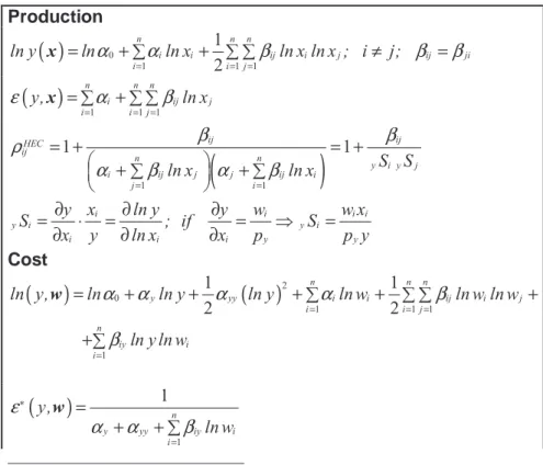
As regards the Translog production and cost functions, it is very difficult, if not impossible, to find something that has not al-ready been written22. However, these functions are shown in Table 5, in order to make proper comparisons with the profit and distance functions.
The profit function was taken from Lau23. Its analytical form is formally similar to that of the production function, with qi in the place of xi, and thus the formulas of ρHECand σHLES are equally similar. Apart from this analogy, the two elasticities have the com-mon feature of being gross.
The distance function was obtained by means of the reduction to a single output of the multi-output function proposed and used by R. Färe and S. Grosskopf, unanimously recognised as experts on the subject24. The reduction to a single output and the elimina-tion of fixed inputs, as well as obviously reducing the number of terms in the function, means that it takes on a significant formal similarity with the cost function. Apart from the presence of inputs
i
x in the place of their unitary costs wi, the difference between it and the cost function is due to the absence of the term αyyln y
( )
2. However, its presence or absence does not influence calculation of21
There are, of course, more sophisticated extensions and variants than those presented here (see, for instance, Nakamura, 1990). However, those in the text are the most fre-quently used.
22
Although it is quite well-known, the only circumstance which is perhaps worth noting here is that there are substantial differences in the formal equality of the formulas of ρHEC and
AUES
σ , which influence their values. In effect, there is nothing which imposes and/or guar-antees that coefficients βij, obtained from the estimates of the cost function, are not signifi-cantly different from those of the production function. This is why the independent variables are different, and why the term βiyln y appears in the equations of the si of the cost func-tion but not in those of the producfunc-tion funcfunc-tion.
23
See Lau 1978, pag. 194.
24
See Grosskopf, Hayes and Hirschberg (1995). It should be recalled that these authors, on page 257, write the function as ln( )1 =α0+αln y....
the partial derivatives (of an additive function in the logarithms) with respect to wi or xi, which are necessary to calculate the elas-ticities of substitution and complementarity. If the uni-product ver-sion of the distance function is accepted, its partial derivatives are a mix of those of the production function (due to the presence of inputs xi) and of those of the cost function (due to the presence of output y). The different values of the elasticities are thus en-trusted to the differing combinations of the variables according to which they are defined25.
Table 5 – Translog Functions
Production
( )
0 1 1 1 1 2 n n n i i ij i j ij ji i i j ln y lnα α ln x β ln x ln x ; i j; β β = = = = +∑ + ∑ ∑ ≠ = x( )
1 1 1 n n n i ij j i i j y, ln x ε α β = = = =∑ +∑ ∑ x(
)
1 1 1 ij 1 ij HEC ij n n y i y j i ij j j ij i j i S S ln x ln x β β ρ α β α β = = = + = + +∑ +∑ i i i i y i y i i i i y y y x ln y y w w x S ; if S x y ln x x p p y ∂ ∂ ∂ = ⋅ = = ⇒ = ∂ ∂ ∂ Cost(
)
( )
2 0 1 1 1 1 1 1 2 2 n n n y yy i i ij i j i i j n iy i i ln y, ln ln y ln y ln w ln w ln w ln y ln w α α α α β β = = = = = + + +∑ + ∑ ∑ + +∑ w(
)
1 1 * n y yy iy i i y, ln w ε α α β = = + +∑ w(
)
1 1 1 1 ij AUES ij n n i iy ij j j jy ij i j i ij c i c j ln y ln w ln y ln w S S β σ α β β α β β β = = = + = + +∑ + +∑ = + i i i c i i c i i i i lnC C w C w x S ; x S ln w w C w C ∂ ∂ ∂ = = ⋅ = ⇒ = ∂ ∂ ∂ 1 1 1 1 ij ii MES ij n n j iy ij i i iy ij j i j ij ii c j c i ln y ln w ln y ln w S S β β σ α β β α β β β β = = = + − = + +∑ + +∑ = + − 1 1 1 1 ij jj MES ji n n i iy ij j j jy ij i j i ij ii c i c j ln y ln w ln y ln w S S β β σ α β β α β β β β = = = + − = + +∑ + +∑ = + −demand function input xi =cost share of input xi
1 n i i i iy ij i i w x ln y ln w C = +α β +∑= β Profit
( )
0 1 1 1 1 2 n n n i i i ij i j ij ji i i i j y w lnG ln ln q ln q ln q ; i j; ; q p α α β β β = = = = +∑ + ∑ ∑ ≠ = = q(
)
1 1 1 ij HLES ij n n i ij i j ij j j i ln q ln q β σ α β α β = = = + +∑ +∑ demand function input xi
( )
1 n i i i ij j j q x ln q G α = β = − +∑ qDistance
( )
0 1 1 1 1 1 2 n n n n y i i i j iy i i i j i ln D y, lnα α ln y α ln x ln x ln x β ln x ln y = = = = = + +∑ + ∑ ∑ +∑ x(
)
(
)
0 1 1 1 1 1 1 2 2 1 2 n n n n y ij i j iy i i j i AEC ij ij n n i iy ij j j j ij i j i ln ln y ln x ln x ln x y ln x y ln x y ln x α α α β β ρ β α β β α β β = = = = = + +∑ +∑ ∑ + ∑ = + + + + ∑ ∑ 1 1 1 ij MEC ij n n j jy ij i i iy ij j i j ii ln y ln x ln y ln x β β ρ α β β α β β = = = + − + +∑ + +∑ 1 1 1 ij jj MEC ji n n i iy ij j j jy ij i j i ln y ln x ln y ln x β β ρ α β β α β β = = = + − + +∑ + +∑(inverse) demand function for inputs xi
( )
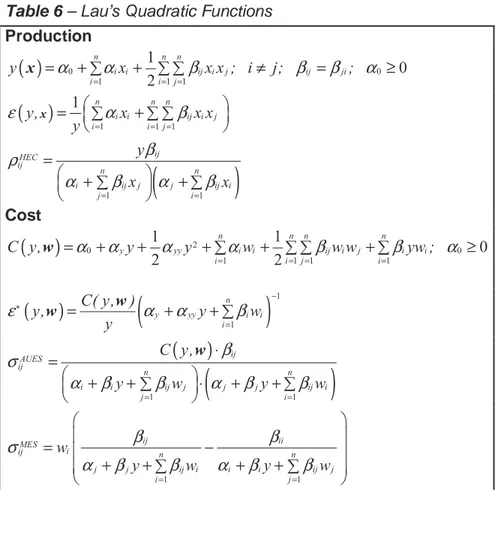
1 1 n i i iy ij j j i i D y, x ln y x x x α β = β ∂ = = + +∑ ∂ x5. Flexible Functional Forms: b) Lau’s Quadratic and Diew-ert’s Generalized Cobb-Douglas, Extended by Magnus
If we compare Lau’s Quadratic production function with Trans-log, we see that the latter repeats its form, with natural rather than logarithmic values. Lau, who is one of the most important contribu-tors to the theory of the profit function, did not formulate any func-tion, of either cost or distance. Both have been proposed by us, exploiting the analogy with Translog, i.e. using its form in natural
eliminates respectively y and C y,w
(
)
from the formulas. Lau states that the production function is “self dual” and thus its convex conjugate, i.e., the profit function, is also quadratic and is written with G q( )
in place of y, and qi in place of xi26. The consequence
– mutatis mutandis – is that the formula of σHLES is formally similar to that of ρHEC.
Table 6 – Lau’s Quadratic Functions
Production
( )
0 0 1 1 1 1 0 2 n n n i i ij i j ij ji i i j y α α x β x x ; i j; β β ; α = = = = +∑ + ∑ ∑ ≠ = ≥ x( )
1 1 1 1 n n n i i ij i j i i j y, x x x y ε α β = = = = ∑ +∑ ∑ x(
)
1 1 ij HEC ij n n i ij j j ij i j i y x x β ρ α β α β = = = +∑ +∑ Cost(
)
2 0 0 1 1 1 1 1 1 0 2 2 n n n n y yy i i ij i j i i i i j i C y, α α y α y α w β w w β yw ; α = = = = = + + +∑ + ∑ ∑ +∑ ≥ w(
)
(
)
1 1 n * y yy i i i C( y, ) y, y w y ε α α β − = = w + +∑ w(
)
(
)
1 1 ij AUES ij n n i i ij j j j ij i j i C y, y w y w β σ α β β α β β = = ⋅ = + + ⋅ + + ∑ ∑ w 1 1 ij ii MES i ij n n j j ij i i i ij j i j w y w y w β β σ α β β α β β = = = − + +∑ + +∑ 26See Lau (1978), p. 194. However, his statement regarding self-duality is not accompanied by any explanation or reference to another publication.
1 1 ij jj MES j ji n n i i ij j j j ij i j i w y w y w β β σ α β β α β β = = = − + +∑ + +∑
demand function for input
(
)
1 n i i i ij j j i C y, x y w w α β = β ∂ = = + +∑ ∂ w Profit
( )
0 0 1 1 1 1 0 2 n n n i i i ij i j i i i j y w G q q q ;q ; p α α β α = = = = +∑ + ∑ ∑ = ≥ q( )
(
)
1 1 ij HLES ij n n i ij j j ij i j i G q q β σ α β α β = = = + + ∑ ∑ qdemand function for input
( )
1 n i i ij i j i G x q q α = β ∂ = = − +∑ ∂ q Distance
( )
1 1 1 1 1 2 n n n n y i i ij i j iy i i i j i D y, α y α x β x x β x y = = = = = +∑ + ∑ ∑ +∑ x( )
(
)
1 1 ij AEC ij n n i iy ij j j jy ij i j i D y, y x y x β ρ α β β α β β = = = + +∑ + +∑ x 1 1 ij ii MEC i ij n n j jy ij i i iy ij j i j x y x y x β β ρ α β β α β β = = = − + +∑ + +∑ ij jj MEC j ji n n i iy ij j j jy ij i x y x y x β β ρ α β β α β β = − + +∑ + +∑ Among the elasticities taken from the distance and cost func-tions, the relationships of formal analogy described above for the same functions in Translog are repeated.
The functions of the generalized Cobb-Douglas form, shown in logarithmic terms for convenience, do not present any especially distinctive features. As the production function is subject to con-stant returns to scale, the equality between ρHEC and ρAEC turns out to be confirmed, as expected (Kim, 2000).
The cost function shown in non-homothetic form is due to Guilkey et al. (1983). The presence of terms ln y and
( )
ln y 2 - as in Translog and GL – means that σAUES loses its formal analogy with ρHEC and reduces the possibility of simplifying the formula. In the σMES formulas, the partial own prime and second derivatives are shown with the symbol d (for reasons of space) and appear in extended form in the Appendix. The presence in the formulas of negative signs in front of the two terms should not mislead read-ers, causing perplexity. That of the first term comes from the sec-ond mixed derivative of the function, whereas the secsec-ond term is annulled by the negativity of its own second derivatives.The demand function of input i is presented in Translog form as the quota of its total cost, multiplying the prime derivative of the cost function by its unitary cost wi.
The normalised profit function, proposed by the writer, does not present any particular difficulty.
Table 7 - Magnus Extended, Diewert’s Generalized Cobb-Douglas Functions Production
(
)
1 1 1 1 0 0 1 n n n n ij i i j j i ij ij ji i j i j ln y lnγ β ln α x α x ; α ; γ ; β ; β β = = = = = +∑ ∑ + ≥ > ∑ ∑ = =( )
1 1 1 n n ij i j y, ε β = = =∑ ∑ = x(
)
2 1 1 1 1 2 ij HEC ij n ij n ij i i j j j i i j j i i i j j x x x x x x β ρ β β α α α α α α = = = − ⋅ + ∑ ∑ + + Cost(
)
( )
(
)
2 0 1 1 1 1 2 y yy n n n ij i i j j iy i i j i lnC y, ln ln y ln y ln w w ln y ln w α α α β α α α = = = = + + + +∑ ∑ + +∑ w(
)
(
)
1 1 n * y yy iy i i y, ln y ln w ε α α α − = = + +∑ w(
)
2 1 1 2 1 2 1 2 i j ij AUES ij n iy ij i i j j i j i i i j j n iy ij j i j i i j j ln y w w w w w ln y w w w α α β σ α β α α α α α α α β α α = = = − ⋅ + + ∑ + ⋅ + ∑ + (
)
2 2 i j ij ii MES i ij i i i j j d w d w w α α β σ α α = − − + (
)
2 2 i i ij jj MES j ji j i i j j d w d w w α α β σ α α = − − + demand function input xi =cost share of input xi
(
)
(
)
1 2 i i i j ij i i i j j yi w x w w w ln y C y, α α β α α α − = + + w Profit( )
0(
)
1 1 n n ij i i j j i j lnG lnα β ln αq α q = = = +∑ ∑ ⋅ + q βdemand function for input
( )
(
)
1 2 n ij i i j i i i j j G x q q q β α α α = ∂ = − = − ∑ ∂ + q Distance( )
1(
)
1 1 n n y ij i i j j i j ln D y, lnγ α ln y− β ln α x α x = = = + +∑ ∑ + x(
)
2(
)
(
)
1 1 1 1 2 ij AEC ij n n ij ij i i j j j i i j j i i i j j x x x x x x β ρ β β α α α α α α = = = − + ∑ ∑ + + (
) (
2)
(
)
1 1 2 ij i i ii MEC ij n n ij ij i i j j i i i i i j j j i i j j x x x x x x x x β α β ρ β β α α α α α α α = = = − + + ∑ ∑ + +(
) (
2)
(
)
1 1 2 ij j j jj MEC ji n n ij ij i i j j j j j i i j j i i i j j x x x x x x x x β α β ρ β β α α α α α α α = = = − + + ∑ ∑ + +inverse demand function for input
( )
(
)
1 2 n ij i i j i i i j j D y, x x x x β α α α = ∂ = = ∑ ∂ + x 6. Final ConsiderationsAt the conclusion of a research which produced in the author a mixture of disappointment and interest – work which he would not have undertaken if he had seen the general picture clearly right from the beginning – some comments may be made. First, al-though admitting the modesty of the aim of the research and of its mathematical and theoretical standard, we hope that the “parade” of the seven inflexible and flexible functional forms, may be useful for formulating evaluations which are not simple but more articu-lated.
A first consideration regards IFF and FFF as separate groups. Due to their functions and correlated elasticities, IFF present solu-tions which may be defined as clear and distinct within their limited scope, as shown by unitary or constant but in any case positive values. For these solutions, inputs are always and only q -complements and p-substitutes. They are clear solutions be-cause, due to their self-dual nature, the rules of economic and mathematical logic proceed along the same lines; and they are dis-tinct because the four functions have specific and proper equation forms. The non-determination of the profit function for the CMC-CES form and the hypothetical conclusions on the elasticity of the distance function are certainly due only to the writer’s limited ca-pacity to face the analytical difficulties which others will doubtless find easy to carry out.
The overall picture of the FFF is very different from that of the IFF, but not less unitary from other aspects. The deliberate aban-don of self-duality between the functions and the acceptance of an approximation as second best, involves more or less similar con-sequences for all functions. Once the equation form of the produc-tion funcproduc-tion has been chosen and defined while respecting estab-lished canons, the others must be “invented”. Emblematic here is the case of the cost function of the functional forms DGL, TL and MEDGCD, of which the first and third have production functions with constant returns to scale. Now, the terms y and y2 were in-serted in the three cost functions in order to have variable econo-mies of size and to presume a priori – and more realistically – vari-able (increasing) average and marginal costs. If this was done by clearly authoritative experts, then it seems to us that the ”invention by analogy” on our part of the cost function for Lau’s Quadratic, in which we introduced y and y2, should not be blamed.
Of the profit functions, three out of four have the mark of the inventors of production functions, i.e., Diewert and Lau. In this
inventions have very different parentage: Färe and Grosskopf for Translog, and the present writer for Lau’s Quadratic.
Secondly, an overall view of the functional forms helps us to assess better and understand the reasons which led econometri-cians to prefer certain functional forms and, within them, to choose the most suitable among the four functions. Among the FFF, the preference for Translog is explained by its generality and the fact that it can be extended27. Its production function is presumed to be neither homogeneous nor homothetic, its elasticities are not con-stant, and technological, physico-natural and social variables may be added without difficulty. As regards the three IFF, readers will not be surprised if the writer views CMC-CES as progress with re-spect to CD and CES-ACMS, at least as regards the variable trends (first increasing, then decreasing) of average and marginal productivities.
Considering the set of four FFF, the cost function is the most frequently applied, and we believe this is because non-homogeneity and non-homotheticity may be assumed a priori (em-pirical data reject homogeneity with increasing frequency), as long as they can be tested a posteriori28.
Application of the distance function still does not seem to have reached the level of the cost and production functions, although – for several reasons - this is definitely to be hoped for. The main reasons are its capacity to treat the multi-output case and to be fruitfully applicable in conditions of limited profitability with respect to ends or means29. The distance function also seems to be the parametric instrument best able to sustain the challenge with non-parametric analysis, which is becoming more popular. The poor application of the profit function is very probably due to competition conditions in the production markets which it must assume. This circumstance is confirmed by the fact that its application covers
27
The preference is not hampered by the danger of falling into the “concavity trap”, a dan-ger shared by other FFF like DGL, which is also largely applied. Some researches regard the checking of the concavity conditions for all data of the available sample as a positive feature of the Translog and DGL functions.
28
From this viewpoint too, Translog is in a better position with respect to the others, be-cause its production function may also sometimes perform better than the cost function in terms of fitting empirical data, and with different but yet significant estimates of the parame-ters.
29
agricultural production, in which the above conditions are judged to be quite satisfied30.
As regards elasticities, we believe that their characteristics and mutual relations have been sufficiently described in the previ-ous Sections. There is only one question remaining open: is Mor-ishima’s or Allen’s form (in which all the others are shown) to be preferred? The writer has reflected on this point for some time and the preparation of this survey reinforced his views, although he is in a minority: with more than two inputs and non-homothetic func-tions, Morishima’s elasticities are more appropriate. For this rea-son, they were calculated and presented together with σAUES and
AEC
ρ . Without going back about fifteen years or so to the words of Blackorby and Russell31, which are still valid, we observe that ex-tension of the application to the distance function of Morishima’s elasticities as operated by Kim (2000, p. 257) may be performed for all the others. The reason for this extension, which does not prevent us from using traditional versions when suitable, is that
MES
σ and ρMEC, together with non-homogeneous (or at most ho-mothetic) production functions and distance functions are, in our opinion, the main analytical tools capable of continuing develop-ment of the parametric theory of production.
Appendix
The derivatives of the MEDGCD cost function in the MES ij σ and MES ji σ formulas are: 1 2 n iy ij i i j i i i j i ln y d w w w α α β α α = = + ∑ +
(
)
2 1 1 2 2 2 n i j ij iy ij i j i i i j j i i j j ij n jy ij j i j i i j j ln y w w w w w d ln y w w w α α β α α β α α α α α α β α α = = − + + ∑ ⋅ + + = ⋅ + ∑ + 2 2 2 1 1 2 n 2 n iy ij iy ij ii i i j i i j j i j i i j j i ln y ln y d w w w w w w α α β α α β α α α α = = = − − ∑ + + ∑ + + jjReferences
ALLEN R.G.D., “Analisi matematica per economisti” (Italian trans. of “Mathematical Analysis for Economists”, London, MacMillan, 1938, by A. Uggé), Milano-Varese, Istituto Editoriale Cisalpino, 1955.
ANTLE J.M., “The structure of U.S. Agricultural Technology”, American Journal of Agricultural Economics, 1984, nov., pp. 414-423.
ANTONELLI G.B., “Sulla teoria matematica dell’Economia Politica”, Pisa, 1886, reprinted in Il Giornale degli Economisti, 1951. ARROW K.J., CHENERY B.H., MINHAS B.S., SOLOW R.M.,
“Capital-Labor Substitution and Economic Efficiency”, Review of Eco-nomics and Statistics, 1961, Vol. 43, no. 3, pp. 225-250. BERTOLETTI P., “Elasticity of Substitution, One More Time: Gross
Versus Net, Direct Versus Inverse Measures”, Working Paper n. 56, November 2001, Università degli Studi di Torino, Facol-tà di Economia, Dipartimento di Scienze Economiche e Finan-ziarie “G. Prato”.
BLACKORBY C.,RUSSEL R.R., “Will the Real Elasticity of Substitu-tion Please Stand Up? (A comparison of the Allen/Urzawa and Morishima Elasticities)”, American Economic Review, 1989, Vol. 79, no. 4, pp. 882-888.
CANTARELLI D., MARANGONI G., CUPELLO L., “Contributo alla teoria della funzione di produzione”, Padova, CEDAM, 1990.
CANTARELLI D.,DI FONZO T.,GIACOMELLO B., “A New Model of an Inhomogeneous Multifactor Production Function”, Rivista In-ternazionale di Scienze Economiche e Commerciali, 1994, Vol. XLI, no. 6-7, Giugno-Luglio, pp. 491-517.
CANTARELLI D., GIACOMELLO B., “Allen’s and Morishima’s
Elastici-ties of Substitution in a VES Inhomogeneous Production Fun-ction: A Comparison”, Giornale degli Economisti e Annali di Economia, 1995, Gennaio-Marzo, pp. 1-24.
CANTARELLI D., “A “Quasi-Dual” Approximation of a
Non-Homothetic Cost Function: Results of a Preliminary Experi-ment”, Rivista Internazionale di Scienze Economiche e Com-merciali, 1999, Vol. XLVI, no. 3, September, pp. 467-497.
CANTARELLI D., “The “Quasi-Dual” Approximation of a Non-Homothetic Cost Function, II: Results of a Further Experi-ment”, Rivista Internazionale di Scienze Economiche e Com-merciali, 2003, Vol. L, no. 1, March, pp. 15-38.
CHAMBERS R., “Applied Production Analysis: A Dual Approach”, 1988, Cambridge, Cambridge University Press.
CORNES R., “Duality and Modern Economics”, 1992, Cambridge,
Cambridge University Press.
DEATON A., “The Distance Function in Consumer Behavior with Applications to Index Numbers and Optimal Taxation”, Review of Economic Studies, 1979, Vol. 46, pp. 391-405.
DIEWERT E., “An Application of the Shephard Duality Theorem: A Generalized Leontief Production Function”, Journal of Political Economy, 1971, Vol. 79, no. 3, pp. 481-507.
DIEWERT E., “Functional Forms for Profit and Transformation Func-tions”, Journal of Economic Theory, 1973, Vol. 6, pp. 284-316. DIEWERT E., “Separability and a Generalization of the Cobb-Douglas Cost, Production and Indirect Utility Functions”, De-partment of Economics, University of British Columbia, 1973. FÄRE R., PRIMONT D., “Multi-Output Production and Duality: Theory
and Applications”, Kluwer Academic Publisher, Boston, 1995. GROSSKOPF S., HAYES K., HIRSCHBERG I., “Fiscal Stress and the
Production of Public Safety: A Distance Function Approach”, Journal of Public Economics, 1995, Vol. 57, pp. 227-296. GUILKEY D.K.,LOVELL K.C.A.,SICKLES R.C., “A Comparison of the
Performance of Three Flexible Functional Forms”, Interna-tional Economic Review, 1983, Vol. 24, no. 3, October, pp. 591-616.
HICKS J.R., “Elasticities of Substitution Again: Substitutes and Complements”, Oxford Economic Papers, 1970, Vol. 22, pp. 289-296.
KIM H.Y.,“The Antonelli versus Hicks Elasticities of Complemen-tarity and Inverse Input Demand Systems”, Australian
Eco-to Theory and Applications, North Holland Publishing Com-pany, Amsterdam, 1978, pp. 134-216.
LOPEZ R.E., “Estimating Substitution and Expansion Effects Using
a Profit Function Framework”, American Journal of Agricultural Economics, 1984, Aug., pp. 358-367.
MCFADDEN D., FUSS M., MUNDLAK Y., “A Survey of Functional Forms in the Economic Analysis of Production”, Ch. II of FUSS
M. and MCFADDEN D. (Eds.), Production Economics: A Dual Approach to Theory and Applications, North-Holland Publish-ing Company, Amsterdam, 1978, pp. 216-268.
MAGNUS I., “Substitution Between Energy and Non-Energy Inputs in The Netherlands 1950-1976”, International Economic Re-view, 1979, Vol. 20, no. 2, June, pp. 465-484.
MORISHIMA M., “Danryokusei riron ni kansuru ni-san no teian (A few suggestions on the theory of elasticity), Keizai Hyoron, 1967, Vol. 16, pp. 144-150 (Section IV, translated from Japa-nese into Italian).
MUNDLAK Y., “Elasticities of Substitution and the Theory of Derived Demand”, Review of Economic Studies, 1968, Vol. 35, pp. 225-236.
NAKAMURA S., “A Nonhomothetic Generalized Leontief Cost Func-tion Based on Pooled Data”, Review of Economics and Statis-tics, 1990, Vol. LXXII, no. 4, pag. 649-655.
PARKS R.W., “Price Responsiveness of Factor Utilization in Swed-ish Manufacturing”, Review of Economics and Statistics, 1971, Vol. LIII, no. 2, May, pp. 129-139.
SATO R.,KOIZUMI T., “On the Elasticities of Substitution and Com-plementarity”, Oxford Economics Papers, 1973, Vol. 25, pp. 44-56.
SEIDMAN L.S., “Complements and Substitutes : The Importance of Minding p’s and q’s”, Southern Economic Journal, 1989, Vol. 56, pp. 183-190.
SHUMWAY C.R., “Supply, Demand, and Technology in a Multipro-duct Industry: Texas Field Crops”, American Journal of Agri-cultural Economics, 1983, Nov., pp. 748-760.
SIDHU S.S.,BAANANTE C.A., “Estimating Farm-Level Input Demand and Wheat Supply in the Indian Punjab Using a Translog Profit Function”, American Journal of Agricultural Economics, 1981, May, pp. 237-246.
SYRQUIN M.,HOLLENDER G., “Elasticities of Substitution and Com-plementarity: The General Case”, Oxford Economic Papers, 1982, Vol. 34, pp. 515-519.
UZAWA H., “Production Functions with Constant Elasticities of Sub-stitution”, 1962, Review of Economic Studies, Vol. 29, pp. 291-299.
UZAWA H., “Duality Principles in the Theory of Cost and
Produc-tion”, International Economic Review, 1964, Vol. 5, no. 2, May, pp. 216-220.
WORKING PAPERS DEL DIPARTIMENTO
1988, 3.1 Guido CELLA
Linkages e moltiplicatori input-output.
1989, 3.2 Marco MUSELLA
La moneta nei modelli di inflazione da conflitto.
1989, 3.3 Floro E. CAROLEO
Le cause economiche nei differenziali regionali del tasso di disoccupazione.
1989, 3.4 Luigi ACCARINO
Attualità delle illusioni finanziarie nella moderna società.
1989, 3.5 Sergio CESARATTO
La misurazione delle risorse e dei risultati delle attività innovative: una valu-tazione dei risultati dell'indagine CNR- ISTAT sull'innovazione tecnologica.
1990, 3.6 Luigi ESPOSITO - Pasquale PERSICO
Sviluppo tecnologico ed occupazionale: il caso Italia negli anni '80.
1990, 3.7 Guido CELLA
Matrici di contabilità sociale ed analisi ambientale.
1990, 3.8 Guido CELLA
Linkages e input-output: una nota su alcune recenti critiche.
1990, 3.9 Concetto Paolo VINCI
I modelli econometrici sul mercato del lavoro in Italia.
1990, 3.10 Concetto Paolo VINCI
Il dibattito sul tasso di partecipazione in Italia: una rivisitazione a 20 anni di distanza.
1990, 3.11 Giuseppina AUTIERO
Limiti della coerenza interna ai modelli con la R.E.H..