The signaling effect of gasoline taxes and its distributional implications

(1)

11 June 2021

TIEZZI, S., & Verde, S. (2017). The signaling effect of gasoline taxes and its distributional implications. In EUI Working Papers (pp. 1-27). Firenze : RSCAS 2017/06 Robert Schuman Centre for Advanced Studies Florence School of Regulation Climate.

This is the peer reviewd version of the followng article:

The signaling effect of gasoline taxes and its distributional implications

Publisher:

Terms of use:

Open Access

(Article begins on next page)

The terms and conditions for the reuse of this version of the manuscript are specified in the publishing policy. Works made available under a Creative Commons license can be used according to the terms and conditions of said license. For all terms of use and more information see the publisher's website.

Availability:

RSCAS 2017/06 Robert Schuman Centre for Advanced Studies Florence School of Regulation Climate This version is available http://hdl.handle.net/11365/1005673 since 2017-07-20T13:46:49Z

(2)

RSCAS 2017/06

Robert Schuman Centre for Advanced Studies

Florence School of Regulation Climate

The signaling effect of gasoline taxes and its

distributional implications

(3)

(4)

_{European University Institute}

Robert Schuman Centre for Advanced Studies

Florence School of Regulation Climate

The signaling effect of gasoline taxes and its distributional

implications

Silvia Tiezzi and Stefano F. Verde

(5)

This text may be downloaded only for personal research purposes. Additional reproduction for other purposes, whether in hard copies or electronically, requires the consent of the author(s), editor(s). If cited or quoted, reference should be made to the full name of the author(s), editor(s), the title, the working paper, or other series, the year and the publisher.

ISSN 1028-3625

European University Institute Badia Fiesolana

I – 50014 San Domenico di Fiesole (FI) Italy

www.eui.eu/RSCAS/Publications/ www.eui.eu

(6)

Robert Schuman Centre for Advanced Studies

The Robert Schuman Centre for Advanced Studies (RSCAS), created in 1992 and directed by Professor Brigid Laffan, aims to develop inter-disciplinary and comparative research and to promote work on the major issues facing the process of integration and European society.

The Centre is home to a large post-doctoral programme and hosts major research programmes and projects, and a range of working groups and ad hoc initiatives. The research agenda is organised around a set of core themes and is continuously evolving, reflecting the changing agenda of European integration and the expanding membership of the European Union.

Details of the research of the Centre can be found on: http://www.eui.eu/RSCAS/Research/

Research publications take the form of Working Papers, Policy Papers, Policy Briefs, Distinguished Lectures, Research Project Reports and Books.

Most of these are also available on the RSCAS website: http://www.eui.eu/RSCAS/Publications/

The EUI and the RSCAS are not responsible for the opinion expressed by the author(s).

Florence School of Regulation Climate

Florence School of Regulation Climate (FSR Climate) is a research group within the Robert Schuman Centre for Advanced Studies. Its goal is to provide a reliable source for information and analysis of EU climate policy and a forum for discussion of research carried out in this area among government officials, academics and industry.

FSR Climate is directed by Xavier Labandeira, Professor of Economics at the University of Vigo and it works in collaboration with the energy and regulatory policy research groups of the Florence School of Regulation.

The opinions expressed in this paper are those of the author(s) and do not represent the views of the European University Institute or any of its subsidiary components.

For more information: http://fsr.eui.eu/climate/

(7)

(8)

Abstract

This paper proposes and tests a better defined interpretation of the different responses of gasoline demand to tax changes and to market-related price changes. Namely, the signaling effect of gasoline taxes is one that impacts on long-run consumer decisions in addition to the incentives provided by tax-inclusive gasoline prices. Our hypothesis is tested using a complete demand system augmented with information on gasoline taxes and fitted to household-level data from the 2006 to 2013 rounds of the US Consumer Expenditure survey. Information on gasoline taxes is found to be a significant determinant of household demand additional to tax-inclusive gasoline prices. The equity implications are examined by contrasting the incidence across income distribution of a simulated $0.22/gallon tax increase to that of a market-related price increase equal in size. The tax increase is clearly regressive, slightly more than the market-related price increase. However, regressivity is by no means a reason to give up gasoline taxes as an instrument for reducing gasoline consumption externalities. Their high effectiveness in reducing gasoline demand implies that small tax increases can substantially improve the environment while minimizing the related distributional effects. Also, gasoline taxes generate revenue that can be used to offset their regressivity.

Keywords

Gasoline taxation, signalling effect, demand systems, conditional cost functions, distributional incidence

(9)

(10)

1

1. Introduction

In the US, carbon dioxide (CO2) emissions from the use of private vehicles make up over one fifth of total greenhouse gas emissions (EPA, 2016). Gasoline taxes can be an effective instrument for curbing CO2 emissions from road transportation (Sterner, 2007), but this potential is far from being fully exploited in the US (Parry and Small, 2005). While generating more revenue than any other commodity tax, both at the federal and State levels, gasoline taxes are very low as compared with those levied in many other countries, notably in Europe (

OECD, 2015

). In recent years, however, given the need to raise extra fiscal revenues and growing concerns about climate change, the option of raising gasoline taxes has received greater consideration in the American public policy debate. In addition, the current phase of low gasoline prices has created favorable conditions for implementing gasoline tax hikes.

Gasoline tax increases remain nevertheless highly unpopular. Public resistance to them is at least partly explained by their adverse distributional effects. In developed economies1_{, gasoline is generally} a necessity good in household consumption. Therefore, gasoline price increases tend to affect the poor more than the wealthy in relative terms. That is, they tend to be regressive. Yet, as much as the distributional incidence of gasoline price increases is a critical parameter for the policymaker, its estimation is to some significant extent dependent on the approach used (Sterner, 2012a, 2012b). At least three dimensions of the models used are relevant in this sense: a) the time horizon, which can determine the measure of consumers’ ability to pay, typically income or total expenditure as a proxy for lifetime income; b) the price elasticities of gasoline demand, which may or may not vary across households; and c) the tax elasticities of gasoline demand, which may or may not differ from the price elasticities. In this paper, we control for these elements within a single empirical framework.

In an application to US household data, our analysis allows for distinct price and tax elasticities of gasoline demand varying across income distribution, and considers two alternative measures of ability to pay, namely annual income and annual total expenditure. Central is the distinction between the responses of gasoline demand to tax changes and to market-related price changes (i.e., related to market forces). There is indeed growing evidence that the first have much bigger impacts on gasoline demand than the second (Davis and Kilian, 2011; Scott, 2012; Baranzini and Weber, 2013; Brockwell, 2013; Li

et al., 2014; Rivers and Schaufele, 2015; Tiezzi and Verde, 2016; Antweiler and Gulati, 2016;

Andersson, 2016). In the literature, two main explanations are provided which hinge on the greater persistence and the greater visibility through media coverage of tax changes relative to market-related price changes. A tax-aversion explanation is also plausible, whereby consumers may react more if they know that the price increase they face is due to a tax increase (McCaffery and Baron, 2006; Kallbekken

et al., 2010; Kallbekken et al., 2011; Blaufus and Möhlmann, 2014). These explanations are not

mutually exclusive and all imply that gasoline taxes are more effective in reducing gasoline demand than standard price elasticities (i.e., estimated without distinguishing between price changes induced by taxation or by the market) indicate. This means that a given reduction in emissions can be achieved through a smaller tax increase, thus one with a less important distributional impact too.

Using microdata from the 2006 to 2013 rounds of the US Consumer Expenditure Survey, we estimate a complete system of demand augmented with information on gasoline taxes. As in Tiezzi and Verde (2016), gasoline taxes are assumed to have a dual nature and, accordingly, changes in their level affect gasoline demand in two different ways. Considering gasoline taxes as a simple component of the gasoline price, gasoline tax changes alter relative prices. At the same time, considering gasoline taxes as a fiscal policy instrument, changes in their level constitute policy signals. These signals affect long-run consumer decisions, such as buying a more fuel-efficient car, changing transportation mode or moving closer to work, which have an impact on gasoline demand. Thus, in the long run, the

1_{In developed economies, the income elasticity of gasoline demand is typically smaller than 1. The same does not apply to} developing economies.

(11)

Silvia Tiezzi and Stefano F. Verde

2 Robert Schuman Centre for Advanced Studies Working Papers

effectiveness of gasoline taxes in reducing gasoline demand is the result of the two effects: the price effect and the signaling effect, respectively. Just as the price effect, the signaling effect may well vary across households, as different households may respond differently to tax policy signals. The signaling effect would then contribute to determining the distributional impact of the tax change. As concerns the modeling of the tax signal, information on gasoline taxes enters our model as a conditioning variable (Pollak, 1969, 1971).

After model estimation, two counterfactual scenarios are simulated for the years 2006 to 2011. In the Tax Scenario, the federal gasoline tax ($0.184/gallon) is raised by $0.22/gallon, which corresponds to a $25/tCO2 carbon tax. In the Market Scenario, a market-related price increase of the same size ($0.22/gallon) is considered. In the Tax Scenario, the impact of the price increase on gasoline demand is given by the sum of the price effect and the signaling effect. In the Market Scenario, only the price effect is in play. We then assess the distributional impacts of the two price increases, which are equal in magnitude but different in nature (policy vs market). Two approaches are used. The welfare effects of the market-related price increase are first derived, as measured by the Compensating Variation. The same approach cannot be used to evaluate the impact of the tax increase due to gasoline taxes entering the model as a conditioning variable. Welfare comparisons across levels of the conditioning variables are indeed not viable (Pollak and Wales, 1979; Pollak, 1989). We thus conduct tax incidence analysis contrasting the tax payments before and after the tax increase across income distribution.

This paper contributes to the literature in two main ways. First, within a structural model, it proposes and statistically tests a better defined interpretation of the different responses of gasoline demand to tax changes and to market-related price changes. Namely, the signaling effect specific to gasoline tax changes is one that impact on long-run consumer choices in addition to the incentives provided by retail tax-inclusive gasoline prices. Second, it analyzes the distributional incidence of gasoline price increases in relation to their nature as tax increases or market-related increases. The findings bear policy implications concerning the environmental effectiveness and the regressivity of gasoline taxes.

The rest of the paper is organized as follows. Section 2 illustrates the model, the simulation scenarios, and the approaches used to assessing the distributional effects. Section 3 presents the data. Section 4 discusses the results. Section 5 concludes.

2. Methodology

2.1 The QAIDS model with gasoline taxes as a conditioning variable

The functional form chosen for our model is the Quadratic Almost Ideal Demand System (QAIDS) of Banks et al. (1997), which generalizes the popular AIDS introduced by Deaton and Muellbauer (1980a). Compared to the AIDS, the QAIDS adds a quadratic term in (the log of) income, which allows for non linear changes in the budget shares following a price or income change. Moreover, the QAIDS easily allows for consumer heterogeneity and conditional demand functions (Pollak, 1969).

In a demand model, conditioning variables usually represent preallocated goods affecting consumption choices over the goods of interest (i.e., those whose demand is modeled). Such goods can be as diverse as durable goods (Deaton, 1981), public goods (Pollak, 1989) or the time available for leisure (Browning and Meghir, 1991). The first to stress the importance of conditional demand functions was Pollak (1969), who noted that if some goods are preallocated in given quantities, they may affect consumer behavior by preventing instant adjustment to the long-run equilibrium. If so, the goods of interest are not statistically separable from the conditioning goods, which then should be controlled for in a regression.

Though they are not goods, gasoline taxes enter our model as a conditioning variable, in addition to being embedded in the gasoline price index. The idea is that the level of gasoline taxes carries

(12)

The signaling effect of gasoline taxes and its distributional implications

European University Institute 3

information which, as the above examples of conditioning variables, both is exogenous to the consumers and affects their consumption choices2_{. The same approach is used in other demand system studies} analysing the effects of different types of information (e.g., Jensen et al., 1992; Chern et al., 1995; Duffy, 1995; Moro et al., 1996; Brown and Lee, 1997). We expect the level of gasoline taxes to influence long-run consumer choices such as purchasing a more fuel-efficient car, changing transportation mode or moving closer to work, which have an impact on gasoline demand. We check for the validity of our approach by testing whether the goods in the demand system are separable from gasoline taxes as a conditioning variable. If gasoline taxes do determine gasoline demand in addition to their capacity as a price component, then they are a conditioning variable and, therefore, are not separable from the goods in the system.

In formal terms, a cost function conditional on the quantities of the goods of interest, , a set of conditioning variables, , and a set of the consumer’s demographic characteristics, , is defined as:

, , , min | , ,

(1)

where is the price vector of the goods of interest, U is the utility function and u is the utility level. The properties of such function are discussed in Pollak (1969), Browning (1983) and Browning and Meghir (1991). The conditional compensated demand functions, , , , , are the derivatives of c with respect to pi, with 1, 2, … , . Defining y as total expenditure on the n goods , … , , the identity

, , , is inverted to derive the indirect utility function , , , . We can then substitute this indirect utility function into the compensated demand functions to obtain the system of uncompensated demands. The QAIDS allows demographic and conditioning variables to affect demands in a theoretically consistent way.

The QAI conditional cost function has the form:

ln , , , ln , , , , ₁ 1

, ,

(2)

where , , is a homogenous-of-degree-one price function, and , , and , , are homogenous-of-degree-zero price functions. Indicating with the vector , … , both z and d for notational convenience, demographics, a time trend and gasoline taxes as a conditioning variable enter as taste-shifters, , in the share equations. To maintain integrability, these shifters are part of the

terms in ln , , , which is specified as a Translog price aggregator function:

ln , ln 1

2 ln ln

(3)

While and are specified as a Cobb-Douglas price aggregator and as a linear function, respectively:

2_{The conditional demand approach does not require an explicit modeling of the conditioning variables, which are given for} the consumers. We can thus ignore how gasoline taxes are determined.

(13)

, ∏ where ∑ ∑

(4)

ln , ln

(5)

Inverting the cost function (2) to obtain the indirect utility function and, then, applying Roy’s identity, we obtain the following uncompensated budget share equation for good i:

ln ln

, 1

, ln ,

(6)

The demand share equation (6) satisfies integrability (i.e., demand is consistent with utility maximization) under the following parametric restrictions:

∑ 1, ∑ 0, ∑ 0, ∑ 0 ∀ , ∑ 0 (Adding-up)

∑ 0 ∀ (Homogeneity) (Symmetry)

(7)

A simple way to check for the presence of nonlinear income effects is to test the null hypothesis that the parameters are zero3_{. Furthermore, Section 3.3 shows the model specification that is actually} estimated to deal with censoring (large proportions of zeros in the dataset) for some of the budget shares.

2.2 The signaling effect of gasoline taxes

Part of the literature dealing with the different responses of gasoline demand to tax changes and to market-related price changes uses models that do not rest on a specific theory of how the first affect demand differently from the second (e.g., Davis and Kilian, 2011; Li et al., 2014; Rivers and Schaufele, 2015; Andersson, 2016). The rest of the literature uses structural demand systems (e.g., Ghalwash, 2007; Scott, 2012; Brockwell, 2013; Tiezzi and Verde, 2016). To interpret the greater responsiveness of gasoline demand to tax changes, this set of studies makes explicit reference to the signaling effect of tax policy (Barigozzi and Villeneuve, 2006). Still, how the signaling effect exactly operates is not

3_{We ran a likelihood ratio test to test the hypothesis that the λ}

i parameters are zero. The test rejected the null hypothesis,

(14)

explained4_{. Thus, with the demand systems just as with the non-structural models, gasoline prices are} usually broken down into the tax component and its complement, which is the tax-exclusive price. The demand responses to equivalent changes in the two price components are then computed and contrasted. In this respect, we follow Tiezzi and Verde (2016) who estimate a demand system but deviate from the literature in specifying that the signaling effect of a tax change is additional to the effects of tax-inclusive price changes, whether these are caused by market forces or indeed reflect a tax change. Accordingly, gasoline taxes enter the model in two fashions: implicitly as a component of the gasoline price index and explicitly as a conditioning variable. The economic meaning of this modeling choice is that the signaling effect of gasoline tax changes is one that impacts on long-run consumer decisions, such as purchasing a more fuel-efficient car, changing transportation mode or moving closer to work, over and above the incentives provided by the variation of tax-inclusive gasoline prices. The literature related to the signaling effect of tax policy, which is thinner than one would expect, gives no definite indications as to whether the signaling effect influences agents’ short- or long-run decisions, or both. Li

et al. (2014), however, provide empirical evidence supporting the long-run interpretation of the

signaling effect. Using US data on newly purchased vehicles and miles travelled, the authors find that the fuel efficiency of the vehicles purchased responds more strongly to gasoline tax changes than to gasoline price changes. By contrast, no differential effect is observed with respect to miles travelled.

2.3 Simulating the price increases and assessing the distributional incidence

The first part of this section illustrates the simulation scenarios of an increase in the federal gasoline tax and of an equivalent market-related gasoline price increase. The second part illustrates how the distributional incidence of the two price increases is assessed.

2.3.1 Scenarios: tax increase vs market-related price increase

After estimating the model, two counterfactual scenarios are simulated for each quarter of the years 2006 to 20115_{. In the Tax Scenario, the federal gasoline tax, which is $0.184/gallon and has not changed} since 2006, is raised by $0.22/gallon. This increase corresponds to a $25/tCO2 carbon tax, which is representative of the carbon tax rates indicated in recent US legislative proposals to reduce national CO2 emissions6_{. In the Market Scenario, a market-related price increase of the same size ($0.22/gallon) is} simulated. In the Tax Scenario, the impact of the price increase on gasoline demand is given by the sum of the price effect and the signaling effect. In the Market Scenario, only the price effect is in play.

Let us define the tax-inclusive gasoline price at time , , as the sum of the tax-exclusive price, , and taxes, , i.e., . The first step to simulate the Tax Scenario is deriving the counterfactual level of the gasoline price index, _, , which incorporates the tax change . At time , omitting the State subscript for notational convenience,

4_{In the literature, the signaling effect tends to be vaguely defined. For example, “[…] rational habits sway consumers to} reduce gasoline consumption more in response to price increases perceived as permanent than to price increases perceived as temporary. Credible permanence gives any price increase an extra kick, and this expands the power of standard economic instruments to reduce gasoline consumption.” (Scott, 2012); “[…] this article will investigate whether the effects of a change in consumer prices differs depending on whether the price change is due to a tax change or a change in producer price. If there is a statistically significant difference in the sense that a tax increase leads to a larger change in consumption than a producer price change, this is referred to as the signaling effect from taxation.” (Brockwell, 2013).

5_{The simulation period ends in 2011 due to a lack of data on gasoline prices (in levels) for more recent years.}

6_{For example, the 2009 Congress bill Raise Wages, Cut Carbon Act (H.R. 2380, 111}th_{Congress) set an initial rate of}

(15)

, , 1

∆

,

(8)

where _, (small letter) is the baseline (historical) price index and _, (capital letter) is the baseline price. Similarly, the counterfactual level of the gasoline taxes, _, , is computed by adding Δ to the baseline level,

, , Δ

(9) Feeding both the counterfactual levels of the gasoline price index and of gasoline taxes to the estimated model, the counterfactual predicted budget shares are obtained. Holding total expenditure fixed, i.e.,

, , , the predicted percentage change in gasoline demand is computed as follows:

, , , , , , , , , , , , (10)

where _, and _, are respectively the predicted baseline and counterfactual gasoline budget shares. The same procedure applies for the simulation of the Market Scenario, with the following two differences: a) is replaced by in (8) (although _, is unchanged since and are equal in size), and b) 0 in (9), as no policy signal is active.

2.3.2 Distributional incidence: welfare changes vs changes in tax payments

In the literature, the distributional incidence of price increases – their degree of progressivity or regressivity – is measured in different ways. In principle, measures of progressivity (or regressivity) based on welfare changes are the most appropriate as welfare changes account for both the higher cost of consumption and the lower level of consumption after a price increase. In practice, this approach is seldom used because it requires the estimation of a complete demand system, which is data demanding and technically nontrivial. For the specific case of tax increases, as opposed to generic price increases, the conventional approach to measuring tax progressivity uses the changes in households’ (or individuals’) tax payments after the tax increase. With this approach, estimating demand changes is all that is needed. The downside of this approach is that potential substitution of other consumption goods for the taxed one is ignored (Remler, 2004). In this sense, a measure of tax progressivity based on changes in tax payments approximates one that is based on welfare changes.

With reference to our Tax Scenario, a measure of tax progressivity based on welfare changes cannot be derived because gasoline taxes enter the model not only as a price variable but also as a conditioning variable. This feature of the model is decisive as welfare comparisons across different levels of the conditioning variables are not viable (Pollak and Wales, 1979; Pollak, 1989)7_{. We thus assess the} distributional incidence of the simulated tax increase based on the changes in households’ tax payments.

By contrast, the distributional incidence of the market-related price increase is assessed based on the Compensating Variations (CVs). The CV is a precise measure of welfare change following a price

7_{The conditional approach assumes that the choices over the commodity space depend on the conditioning variables –} gasoline taxes in our case. The conditional preference ordering does not allow welfare comparisons between alternative situations (combinations) of prices and conditioning variables, but only of alternative price situations given the same values of the conditioning variables.

(16)

change, defined as the minimum monetary amount by which a consumer would have to be compensated to be as well off as before the price change. Formally, indicating with the base welfare level at time 0, that is, the welfare level in the base period before any price change, the CV is

, ,

(11)

where , is the minimum cost of reaching at prices , and , is the minimum cost of reaching utility at the price vector .

To calculate the CVs, we use the True Cost of Living index numbers (TCOLs) (Deaton and Muellbauer, 1980b). A TCOL index number is the ratio between the cost of achieving a given level of economic welfare after a price change and the cost of achieving the same level of economic welfare before the price change8_{. That is, using the same notation as for the CV above, the TCOL index is}

, ,

(12)

The CV and the TCOL index are clearly related to one another9_{. If the cost function in the base period} is equal to 1, i.e., , 1, the relationship between the CV and the TCOL simply is

1

(13)

It follows that ln ln 1 . We exploit this result to compute the CVs. Using the QAIDS conditional cost function in (2), the QAIDS expression for ln is first derived. Then, setting the cost function in the base period equal to 1 by normalizing all prices to unity, the CVs are retrieved. In formal terms (Martini, 2009)10_,

ln ln ₁ 1 ln ₁ 1

(14)

For , 1, (14) becomes11

8_{TCOLs are a more accurate measure of the welfare change following a price change than Laspeyres index numbers. TCOLs} allow for substitution possibilities in the bundle of goods consumed holding utility constant, while Laspeyres index numbers assume that the same bundle of goods is purchased before and after the price change.

9_{From the definitions of CV and TCOL,}

0, 0 1 .

10_{The vectors and are dropped from the equations for presentational convenience.}

11_{When all relative prices are set to unity, the price functions} _and _{are equal to one and ln} _{. This} parameter, however, is usually set to zero (Banks et al., 1997).

(17)

ln ln ₁ 1

(14b)

Setting , where is total expenditure in the base period, the CVs are obtained:

1

(15)

Finally, the CVs that correctly measure the welfare effects of the simulated gasoline price increase ($0.22/gallon) over time are the differences between the counterfactual CVs and the baseline CVs. The former are the CVs obtained by increasing the historical gasoline prices by $0.22/gallon. The latter are the CVs resulting from historical price variations (i.e., observed inflation). Thus, first both the counterfactual CVs and baseline CVs are calculated as per above, then the difference between the two is taken.

2.3.3 Distributional incidence: income vs total expenditure as a measure of ability to pay

When assessing the regressivity of a price increase, annual income is not the only variable that can be used to rank agents (here, households) by economic welfare level and to quantify the impacts in relative terms. For these two purposes, an important part of the literature estimating the regressivity of gasoline price increases uses annual total expenditure as a measure of ability to pay. The stated rationale for preferring total expenditure to income is that the former is less volatile from one year to another and that, drawing on Friedman’s permanent income theory of consumption (Friedman, 1957), annual total expenditure can be taken as a proxy for lifetime income12_{. However, inasmuch as the distribution of} total expenditure in a given year is more uniform than that of income, as is generally the case, the price increase necessarily results less regressive if the first is used instead of the second. The difference can be substantial (Sterner, 2012a, 2012b). To control for this aspect, we assess the distributional impact of each type of simulated price increase (the tax increase and the market-related price increase) twice, using the two alternative measures of ability to pay.

3. Data and model estimation

3.1 Households’ economic variables and demographics

The US Consumer Expenditure Survey (CE) produced by the Bureau of Labour Statistics (BLS) is the main data source for our application. We use microdata of the quarterly Interview Survey (IS) from eight rounds of the CE: from 2006 to 201313_{. Each CE round has five IS cross-sections: one per calendar} quarter, including the first of the following year14_{. We thus draw on 40 cross-sections, though not all the} observations available (each cross-section has approximately 6,000 observations) are used for estimating the model. This is fitted to a subset of over 83,000 observations: those for which information

12_{Chernick and Reschovsky (1992, 1997, 2000) and Teixidó and Verde (2016) provide arguments and evidence that question} this approach.

13_{See Chapter 16 of the BLS Handbook of Methods for a description of the CE.}

14_{The IS is a panel rotation survey. Each panel is interviewed for five consecutive quarters and then dropped from the survey} and replaced with a new one.

(18)

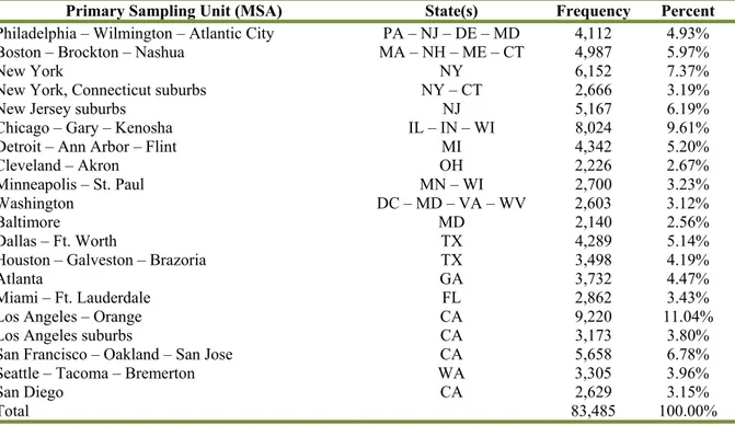
on the Primary Sampling Unit (PSU) is available in the public-use microdata files15_{. We use this subset} because the correspondence between the PSUs and the Metropolitan Statistical Areas (MSAs) of the CPI statistics allows us to exploit the variation of MSA-specific price indices16_{. The resulting sample} spans 93 months, from April 2006 to December 2013, and 20 PSUs/MSAs (see Tables A1 and A2, in the Appendix).

In the IS datasets, each household’s expenditures, which refer to the three months before the interview, are classified into 60 consumption categories. Our system of demand only considers current expenditures (durables and occasional purchases are ignored), corresponding to 40 of the 60 categories. Specifically, the model is estimated for the following shares of total current expenditure:

1. Food at home 2. Electricity 3. Natural gas 4. Other home fuels 5. Gasoline

6. Public transportation 7. Other expenditures

where: Food at home is the total expenditures for food at grocery stores (or other food stores) and food prepared by the consumer unit on trips; Other home fuels is the sum of expenditures on fuel oil, non-piped gas and other fuels (heating fuels); Gasoline comprises expenditures on gasoline, auto diesel and motor oil, but it virtually coincides with gasoline expenditure17_{; Public transportation is the sum of the} fares paid for all forms of public transportation, including buses, taxis, coaches, trains, ferries and airlines.

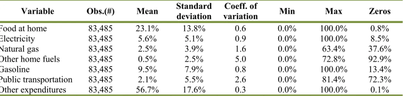
Table 1 shows summary statistics of these expenditure shares as they appear in the sample. On average, Food at home accounts for 23.1% of total current expenditure, followed by Gasoline and

Electricity, which represent 9.5% and 5.6%, respectively. The residual expenditure aggregate, namely Other expenditures, represents 56.7% of total current expenditure. The coefficients of variation indicate

that variability is greatest for Other home fuels, Public transportation and Natural gas, in this order. Large proportions of households reported zero expenditure for these categories (see the shares in the last column of Table 1). Consumption of the respective goods or services is indeed conditional on certain prerequisites, such as the possession of specific appliances or high substitutability between private and public means of transportation, which may not be there for many households.

15_{Only “A”-size PSUs are identified in the public-use microdata files. “A” PSUs are Metropolitan Statistical Areas with a} population greater than 1.5 million.

16_{State-specific price indices are not available at the required disaggregation level.}

(19)

Table 1 – Summary statistics of the budget shares.

Variable Obs.(#) Mean Standard _deviation _variationCoeff. of Min Max Zeros

Food at home 83,485 23.1% 13.8% 0.6 0.0% 100.0% 0.8%

Electricity 83,485 5.6% 5.1% 0.9 0.0% 100.0% 8.5%

Natural gas 83,485 2.5% 3.9% 1.6 0.0% 63.4% 37.6%

Other home fuels 83,485 0.5% 2.5% 5.0 0.0% 72.8% 92.9%

Gasoline 83,485 9.5% 7.9% 0.8 0.0% 100.0% 13.4%

Public transportation 83,485 2.1% 5.5% 2.6 0.0% 81.4% 72.3% Other expenditures 83,485 56.7% 17.6% 0.3 0.0% 100.0% 0.1% Different types of demographic characteristics are extracted from the IS dataset. Descriptive statistics of demographic variables included in the model, as well as of both total expenditure and income, are reported in Table 2. Households are classified by a set of six dummy variables which identify the following types: a) Single; b) Husband and wife; c) Husband and wife, with the oldest child under 6 (years old); d) Husband and wife, with the oldest child between 6 and 17; e) Husband and wife, with the oldest child over 17; f) All other households. Households’ location is captured through four dummy variables, one for each of the Census-defined regions, i.e. Northeast, Midwest, South and West. A dummy variable brings in information on the composition of earners in the household: it takes the value 1 if both the reference person and the spouse are income earners; 0, otherwise. A categorical variable classifies the education level of the household’s reference person in nine levels. The model also controls for the number of vehicles (cars, trucks and vans) owned by the household as well as for the age of the reference person.

Table 2 – Summary statistics of socio-demographics, total expenditure, income.

Variable Obs.(#) Mean Standard _deviation Min Max

Single 83,485 0.28 0.45 0 1

H&W 83,485 0.19 0.39 0 1

H&W, oldest child <6 83,485 0.05 0.22 0 1

H&W, oldest child 6-17 83,485 0.13 0.33 0 1

H&W, oldest child >17 83,485 0.08 0.27 0 1

All other households 83,485 0.27 0.44 0 1

Age of reference person 83,485 49.3 16.8 16 87

Northeast 83,485 0.27 0.44 0 1

Midwest 83,485 0.21 0.41 0 1

South 83,485 0.24 0.42 0 1

West 83,485 0.29 0.45 0 1

Composition income earners 83,485 0.22 0.42 0 1

Education of reference person* 83,485 5.4 1.82 1 9

Number of vehicles 83,485 1.51 1.12 0 10

Total current expenditure, $ 83,485 7,142 6,974 9 324,561

Total expenditure, $ 83,485 13,553 11,795 17 350,481

Disposable income, $ 83,485 71,958 68,867 0 802,242

* 1 “Never attended school”, 2 “1st_{through 8}th_{grade”, 3 “9}th_{through 12}th_{grade”, 4 “High school graduate”, 5}

“Some college, less than college graduate”, 6 “Associate’s degree”, 7 “Bachelor’s degree”, 8 “Master’s degree”, 9 “Professional/Doctorate degree".

3.2 Price indices and gasoline taxes

Insufficient price variation is a common problem when estimating demand models with cross-sectional data and price indices. We avoid this issue by using monthly indices varying by MSA, which taken

(20)

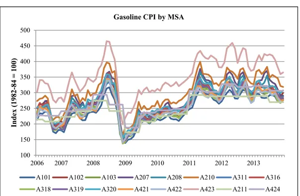
together exhibit sufficient time and spatial variation18_{. Another potential problem is some degree of} inaccuracy in the correspondence between demand and price data. This issue does not arise in our application because the price indices, also produced by the BLS, follow the same classification as that of household expenditure. The BLS uses the CE to periodically revise the expenditure weights of the Consumer Price Index (CPI). There is, thus, perfect correspondence between the expenditure aggregates of the IS and the respective CPI statistics. Table A3, in the Appendix, shows summary statistics of the price indices and of gasoline taxes. Focusing on gasoline prices, Figure 1 pictures the swings of the MSA-specific gasoline price indices over the sample period.

Figure 1 – MSA-specific gasoline CPIs over the sample period.

Note: For the legend of the MSA codes, see Table A2, in the Appendix.

18_{As price indices by MSA are not available for Other home fuels nor for Public transportation, the corresponding US indices} are used in these two cases.

100 150 200 250 300 350 400 450 500 2006 2007 2008 2009 2010 2011 2012 2013 Index (1982-8 4 = 100)

Gasoline CPI by MSA

A101 A102 A103 A207 A208 A210 A311 A316 A318 A319 A320 A421 A422 A423 A211 A424

(21)

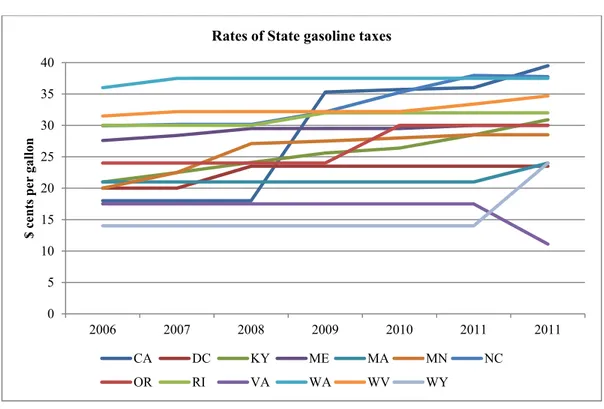
Figure 2 – Most variable rates of State gasoline taxes over the sample period.

In the US, three layers of taxes apply to consumption of gasoline and auto diesel, namely, federal taxes, State taxes and local taxes. The federal tax on gasoline is $0.184/gallon and has not changed since 2006. By contrast, State taxes can differ significantly from one State to another and they are occasionally subject to revisions. The data used on State gasoline taxes are published by the Federal Highway Administration. Local taxes are not considered due to a lack of information, but they are a minor component of the final price. Moreover, to estimate the model, gasoline taxes are adjusted for inflation using the national CPI. Importantly, Figure 2 shows how infrequent changes in gasoline tax rates are19 and that these changes are virtually always increases rather than decreases. This fundamental difference between the dynamics of gasoline taxes and that of gasoline prices provides a compelling explanation for the greater responsiveness of gasoline demand to tax changes relative to price changes.

3.3 Model estimation

To deal with censoring of the dependent variable (the budget shares), we use the two-step estimator introduced by Shonkwiler and Yen (1999)20_{. The procedure involves probit estimation in the first step} and a selectivity-augmented equation system in the second step. The augmented system of equations, which is estimated with Maximum Likelihood, has the following form21_:

19_{Those in the graph are the rates of State gasoline taxes exhibiting the greatest variation over the sample period.}

20_{Shonkwiler and Yen (1999), Yen, Lin and Smallwood (2003), and Yen and Lin (2006) provide useful literature reviews on} estimation procedures for censored demand systems.

21_{A different two-step procedure, developed by Heien and Wessells (1990), has often been used in applied demand analysis} to address the problem of estimating systems of equations with limited dependent variables. West and Williams (2004, 2007) are two studies adopting this procedure. However, as stated by Shonkweiler and Yen (1999), “the Heien and Wessells procedure is built upon a set of equations which deviate from the unconditional mean expression for the conventional censored dependent variable specification”. Instead, Shonkweiler and Yen’s procedure (1999) adopted in this study provides a consistent two-step estimator.

0 5 10 15 20 25 30 35 40 2006 2007 2008 2009 2010 2011 2011 $ cen ts p er gallon

Rates of State gasoline taxes

CA DC KY ME MA MN NC

(22)

Φ , ,

(16) where is the observed expenditure share for good i; is a vector of exogenous variables; is the parameter vector; is the vector containing all parameters in the original demand system (6);

is the heteroscedastic error term; and Φ are the standard normal probability density function (pdf) and its cumulative distribution function (cdf), respectively; and is the unknown coefficient of the correction factor of the i-th equation in the second step.

The dependent variable in the first-step probits is the binary outcome defined by the expenditure in each good. The predicted pdf and cdf from the probit equations are included in the second step of the procedure (Yen, Lin and Smallwood, 2003). The exogenous variables used in the first-step probits are total expenditure, a linear time trend and the set of demographic and geographic variables in the original demand system (6), which are defined in the previous section. As for the second-step estimates, Homogeneity and Symmetry are imposed through parametric restrictions, while Adding-up is accomodated by dropping the equation for the Other expenditures aggregate22_.

Economic theory also requires the matrix of Slutzky substitution effects to be negative semi-definite. This property is satisfied by the data. Second-step estimated coefficients are shown in Table A4, in the Appendix. Moreover, since the estimated elements of the second-step conventional covariance matrix are inefficient, we empirically calculate the standard errors of the elasticities using nonparametric bootstrapping (with 500 replications).

4. Results

This section illustrates the results of our analysis in the following order. We first check for the non- separability of gasoline taxes from the goods in the demand system, which is the key feature of the model’s specification. Estimation results concerning the predicted budget shares and the demand elasticities are subsequently presented, with a special focus on the patterns of the price elasticities and the tax elasticities of gasoline demand across income levels. Finally, the distributional impacts of the two types of simulated gasoline price increases are examined.

4.1 Test of gasoline taxes’ separability

If gasoline taxes affect consumer preferences over the goods in the demand system, ignoring this dependence would result in biased estimates. Browning and Meghir (1991) demonstrate that the conditional cost function approach is most convenient for modeling such dependence. The authors point to several of its advantages. One such advantage is that we can test for weak separability without specifying the structure of the preferences for the goods that are separable under the null hypothesis. A second one is that the conditional cost function approach does not require an explicit structural model for the conditioning variable. Thirdly, testing for weak separability of the goods of interest from the conditioning variables is simple. It boils down to testing whether the conditioning variables should be jointly excluded from the set of explanatory variables.

Following Browning and Meghir (1991), our test of separability of gasoline taxes from the goods of interest consists of a Likelihood Ratio (LR) test in which we compare a restricted model where the budget share equations (6) depend on gasoline taxes (after controlling for prices, total expenditure and

22_{Though the Adding-up restriction holds for the latent expenditure shares, it does not hold for the observed shares. To} address this problem we adopt the approach suggested by Pudney (1989). It consists of estimating n – 1 equations using the two-step procedure together with an Adding-up identity 1 ∑ defining the residual expenditure category as the difference between total expenditure and expenditure on the first n - 1 goods and treating the nth_{good as a residual}

one with no demand of its own. Elasticities for this residual good, if necessary, can be computed using this Adding-up identity.

(23)

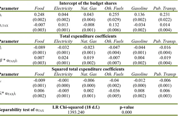
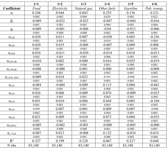
14 Robert Schuman Centre for Advanced Studies Working Papers demographic variables) with an unrestricted model where all tax coefficients are equal to zero. Under the null hypothesis that the unrestricted model holds, the test statistic follows a Chi-squared distribution with 18 degrees of freedom23_{. Table 3 reports all the estimated coefficients relevant to gasoline taxes as} well as the result of the LR separability test. The intercept coefficients are statistically significant in all equations. And the coefficients of the interactions both with total expenditure and squared total expenditure are significant in most equations. As to the LR test, the Chi-squared test statistic allows us to reject the null hypothesis of gasoline taxes’ separability.

Table 3 – Separability test of gasoline taxes: selected QAIDS parameter estimates.

Intercept of the budget shares

Parameter Food Electricity Nat. Gas Oth. Fuels Gasoline Pub. Transp.

αi 0.248 0.044 0.043 0.255 0.136 0.231

(0.002) (0.002) (0.004) (0.029) (0.002) (0.022) αi,TAX -0.007 0.013 -0.008 0.132 -0.034 0.014

(0.003) (0.001) (0.001) (0.006) (0.002) (0.004)

Total expenditure coefficients

Parameter Food Electricity Nat. Gas Oth. Fuels Gasoline Pub. Transp.

βi -0.089 -0.032 -0.023 -0.047 -0.044 -0.016

(0.001) (0.001) (0.001) (0.004) (0.001) (0.004)

(β * αTAX)i _(0.003)0.007 _(0.001)0.024 _(0.002)0.019 _(0.007)-0.007 _(0.002)0.004 _(0.004)-0.019

Squared total expenditure coefficients

Parameter Food Electricity Nat. Gas Oth. Fuels Gasoline Pub. Transp

λi -0.009 -0.001 -0.006 -0.04 -0.012 -0.006

(0.001) (0.000) (0.000) (0.002) (0.000) (0.001)

(λ* αTAX)i _(0.002)0.006 _(0.001)-0.005 _(0.001)0.002 _(0.005)-0.036 _(0.002)0.008 _(0.003)0.006

Separability test of αTAX LR Chi-squared (18 d.f.)_1393.240 p-value _0.000

Note: Robust standard errors in brackets.

4.2 Estimation results

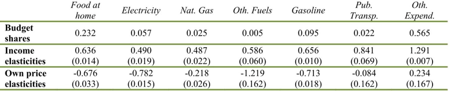
Table 4 presents the predicted budget shares calculated at sample mean values together with the income elasticities and the compensated (Hicksian) price elasticities (also at sample mean values).

23_{The LR test involves 18 restrictions: 6 on the intercepts; 6 on the interactions of taxes and total expenditure; 6 on the} interactions taxes squared and total expenditure.

(24)

Table 4 - Predicted budget shares, income elasticities and compensated price elasticities at sample mean values.

Food at

home Electricity Nat. Gas Oth. Fuels Gasoline

Pub. Transp. Oth. Expend. Budget shares 0.232 0.057 0.025 0.005 0.095 0.022 0.565 Income elasticities (0.014) 0.636 (0.019) 0.490 (0.022) 0.487 (0.060) 0.586 (0.010) 0.656 (0.069) 0.841 (0.007) 1.291 Own price elasticities -0.676 (0.033) -0.782 (0.015) -0.218 (0.026) -1.219 (0.162) -0.713 (0.018) -0.084 (0.162) 0.234 (0.167) On average, gasoline expenditure accounts for almost 10% of households’ budgets, the second highest share among the goods considered in our demand system. In general, the predicted budget shares calculated at sample mean values are very close – as one would expect – to the respective sample mean values (Table 1). The second row in the same table indicates that none of the goods in the model (except for the aggregate Other expenditures) is a luxury good. Demand for public transportation exhibits the largest income elasticity (0.84), a result most likely explained by the heterogeneity of the relative aggregate24_{. Among the energy goods, gasoline is the one with the largest response to income changes} (0.65). As regards the demand responses to price changes, the (long-run) price elasticity of gasoline demand is also high (-0.71), but not too dissimilar from the estimates in other studies fitting demand systems to pooled cross-sectional US data25_.

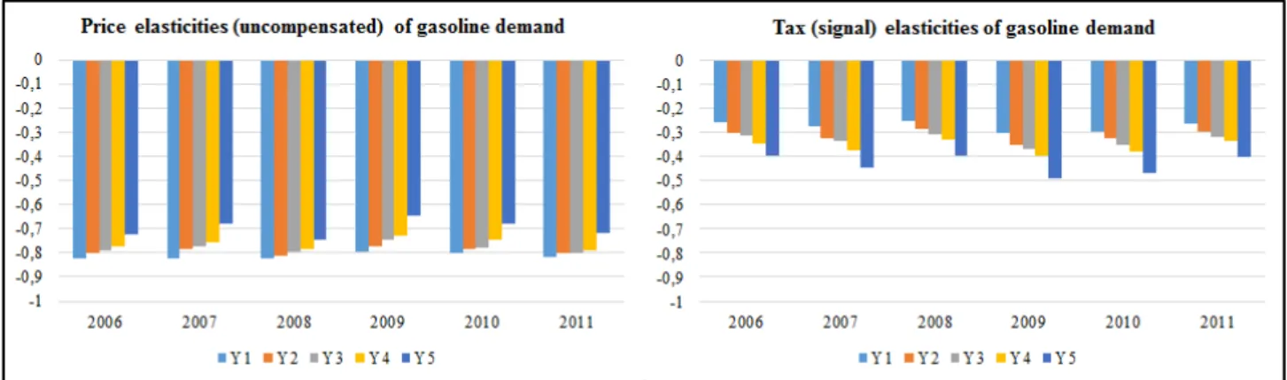
We now focus on the patterns of the mean price elasticity and of the mean tax elasticity of gasoline demand across income distribution26_{. These patterns are of special interest because they are relevant to} the comparative distributional analysis of tax increases versus market-related price increases carried out in the next Section. The left graph in Figure 3 shows the price elasticities of gasoline demand at sample mean values within the (year-specific) income quintiles. For all years, price elasticities decrease (in absolute value) with income level. This result is in line with those of several studies finding that gasoline demand of lower income households is on average more price responsive than that of better-off ones (West, 2004, 2005; West and Williams, 2004; Small and Van Dender, 2007; Wadud et al., 2010a; Liu, 2014). Other studies, however, identify different and even opposite relationships between the price elasticity of gasoline demand and income27_.

24_{As specified in Section 3.1, Public transportation includes the fares paid for buses, taxis, coaches, trains, ferries and} airlines.

25_{For example, in Oladosu (2003), the mean compensated price elasticity of gasoline demand is -0.70 for the third-oldest} owned vehicle and -0.36 for the oldest; in West and Williams (2004), the mean elasticity is -0.73 for the first total expenditure quintile and -0.18 for the fifth; in West and Williams (2007), the range is -0.75 to -0.27 for single-adult and two-adult households, respectively.

26_{For each year, households are sorted by disposable income per adult equivalent. The new OECD equivalence scale is used,} according to which the head of household weighs 1, all other household members aged over 13 weigh 0.5 each, and those under 14 weight 0.3 each.

27_{Kayser (2000), Hughes et al. (2008), Spiller and Stephens (2012) and Gillingham (2014) find the gasoline demand of} wealthier households to be more price elastic. Wadud et al. (2008, 2009, 2010b) find the price elasticities to be highest at the bottom and at the top of the income distribution, while Hausman and Newey (1995), Brännlund and Nordström (2004) and Frondel et al. (2012) do not find statistically significant differences in price elasticities across income levels.

(25)

Figure 3 – Price and tax elasticities of gasoline demand at sample mean values, by year and income quintile.

This heterogeneity of outcomes may be due to multiple factors affecting gasoline demand. On the one hand, lower income households are likely to be more responsive to a gasoline price increase as their lower budgets imply that the income effect is stronger. On the other, gasoline demands of wealthier households may be more responsive to gasoline tax increases, which can be regarded as persistent price increases. The above literature may find conflicting evidence because it makes no distinctions in this respect. The right graph in Figure 3 shows our estimated elasticities of gasoline demand to information on gasoline taxes28_{by income level. In contrast to the price elasticities, which get smaller with income,} the tax elasticities increase with income. This result is consistent with the hypothesis that tax increases affect long-run consumer decisions, including notably investment in more fuel-efficient cars29_{. The} reasoning is that (while wealthier people are less responsive to market-related price changes because they are less affected) tax changes, which are persistent price changes, must be determinants of decisions that both impact on gasoline demand and that wealthier people are more likely to make. Buying a new car – a more fuel-efficient one in the case of a tax increase – is the most obvious decision fitting these two conditions.

4.3 Simulation results: distributional analysis

In this section, we assess the distributional incidence – the degree of regressivity – of the two types of simulated gasoline price increases. First, however, let us recall the relevant specificities of the two simulation scenarios. In the Tax Scenario, the federal gasoline tax is raised by $0.22/gallon. In the Market Scenario, a market-related price increase of the same size is simulated. In the Tax Scenario, the impact of the price increase on households’ gasoline demands is given by the sum of the price effect and the signaling effect. In the Market Scenario, only the price effect is in play. For the Tax Scenario, welfare changes caused by the tax increase cannot be derived, but approximations of the welfare impacts are provided by the changes in households’ tax payments. The distributional incidence of the tax increase is thus based on economic impacts calculated in this way. By contrast, the distributional incidence of the market-related price increase is more accurately quantified by the CVs.

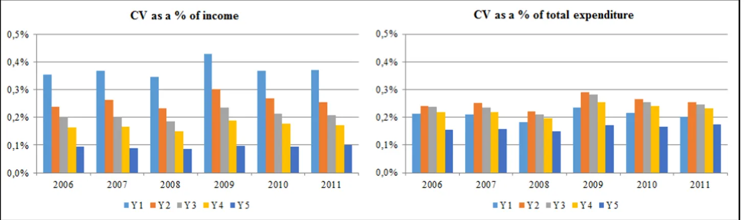
Beginning with the Market Scenario, the left graph in Figure 4 shows, for each of the years considered, the mean CV as a proportion of income, by income quintile. For all years, the emerging patterns indicate that the simulated price increase is clearly regressive. On average, the welfare loss for

28_{The elasticity to information on gasoline taxes only includes the signaling effect of a tax change, not the price effect as} previously defined.

29_{There is ample evidence that gasoline price changes affect the fuel economy of newly purchased cars. For example, Busse} et al. (2013) find that a $1 increase in the gasoline price leads to a 21.1% increase in the market share of the highest fuel economy quartile of cars and a 27.1% decrease in the market share of the lowest fuel economy quartile of cars.

(26)

the households in the first income quintile is in relative terms around four times as big as that suffered by the households in the top quintile30_{. Though differences in welfare impacts over time are generally} modest, slightly smaller effects and slightly bigger effects are observed for the years 2008 and 2009, respectively. These years correspond to the maximum and the minimum levels of the gasoline price path over the simulation period. Hence, the simulated price increase represents respectively smaller and greater percentage increases of the baseline (historical) prices.

Figure 4 – CV as a % of income (tot. expend.) at sample mean values, by year and income (tot. expend.) quintile.

Taking the lifetime approach, by using total expenditure, instead of disposable income, as a measure of ability to pay (both for ranking the households and for expressing the welfare effects in relative terms), results in a partially different picture. The right graph in Figure 4 shows the results obtained. Compared to those in the left graph, the effects are smaller in magnitude for the first quintiles (across years), similar for the second quintiles, and bigger for the others. This is because on average total expenditure is smaller than income, but the converse is true for the poorest. More interestingly, while overall the distributional impact remains regressive, the degree of regressivity is significantly lessened, with the central quintiles bearing the largest burdens31_{. This difference is due to the fact that the distribution of total expenditure} is more uniform than that of income.

The above results are largely comparable to those in West and Williams (2004), which to our knowledge is the only US study estimating the distributional incidence of a gasoline price increase based on welfare effects. Using a demand system approach and CE data from 1996 to 1998, West and Williams (2004) find that the Equivalent Variation (EV) following a gasoline price increase of about $1.00/gallon (an increase five times as big as that considered here) would have ranged -3.01% to -1.60% of total expenditure. Above all, the distributional incidence of the price increase is very similar to that emerging from our application when using total expenditure as a measure of ability to pay.

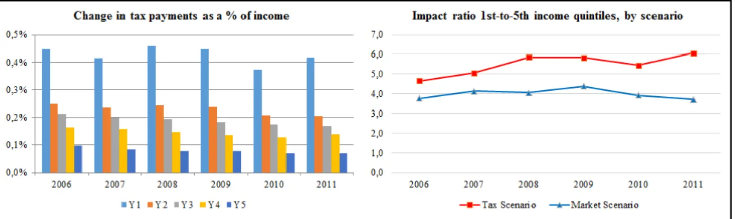
Turning to the Tax Scenario, the left graph in Figure 5 depicts the distributional incidence of the tax increase based on the changes in tax payments as a proportion of income32_{. The magnitude of the effects} is similar to that of the CVs in the Market Scenario. Because of the signaling effect, gasoline demand decreases by greater amounts in the Tax Scenario than in the Market Scenario33_{. However, in the Market} Scenario, the greater welfare losses related to the higher cost of gasoline consumption are partly offset

30_{Table A5, in the Appendix, shows the values of the CVs in absolute terms. Tables A7 and A8 show the corresponding} values of disposable income and of total expenditure, respectively.

31_{This type of result is very common in the literature, since Poterba’s (1991) seminal paper showing the difference in terms} of distributional incidence between using income or total expenditure as measures of ability to pay.

32_{Table A6, in the Appendix, shows the values of the changes in tax payments in absolute terms.}

(27)

18 Robert Schuman Centre for Advanced Studies Working Papers by the welfare gains related to the consumption of gasoline substitutes. In the Tax Scenario, the changes in tax payments do not take this substitution effect into account.

Figure 5 – Left graph: Change in tax payments as a % of income, by year and income quintile;

Right graph: Impact ratio 1st_-to-5th_{income quintiles, by scenario.}

Finally, though a direct comparison is not perfect given the use of different measures of economic impact, the right graph in Figure 5 shows that the tax increase is slightly more regressive than the market-related price increase (by simply comparing the mean impacts for the bottom and top income quintiles). The fact that on average price elasticities decrease (in absolute value) with income while the tax elasticities increase, as previously shown, underlies this result.

5. Conclusions

A growing empirical literature finds that gasoline tax changes have much greater impacts on gasoline demand than equal-in-size market-related price changes. The persistence of tax changes and their salience (through media coverage) are the explanations most frequently provided for this observed outcome. Some studies make explicit reference to the signaling effect of tax policy (Barigozzi and Villeneuve, 2006), but do not go as far as specifying how the signaling effect of gasoline taxes may operate. We take things a step further in positing and testing, within a structural demand system fitted to US data, that the signaling effect of a tax change is additional to the effects of tax-inclusive price changes. The idea is that the signaling effect of gasoline tax changes is one that impacts on long-run consumer decisions, such as purchasing a more fuel-efficient car, changing transportation mode or moving closer to work, over and above the incentives provided by the variations in tax-inclusive gasoline prices. We find evidence corroborating this hypothesis. Firstly, gasoline taxes turn out to be a statistically significant determinant of household demand additional to gasoline prices. Secondly, while the estimated mean price elasticity of gasoline demand decreases (in absolute value) with income, the tax elasticity increases. This result is consistent with our hypothesis on the signaling effect inasmuch as wealthier households more effectively reduce gasoline demand through long-run decisions, notably by buying more fuel-efficient vehicles.

In the US, gasoline price increases are clearly regressive according to our simulations. While much more effective in reducing gasoline demand, tax increases appear to be slightly more regressive than market-related price increases, owing to the said difference in demand responses. Secondary is the role of demand response in determining regressivity, which in the first place depends on the pattern of gasoline consumption across income distribution. By contrast, much more substantial is the difference in outcomes if total expenditure, instead of income, is used as a measure of ability to pay, demonstrating the relevance of this methodological choice (criticized by some authors). If total expenditure is used, the households in the middle of the income distribution – and not the poorest – bear the largest burdens.

(28)

Gasoline taxes are an indispensable instrument for cost-effectively reducing gasoline consumption and, hence, the series of negative externalities (global and local) associated with it. Gasoline tax increases are regressive, but this is by no means a reason to give them up – we could not overemphasize this point. The high effectiveness of gasoline taxes in reducing gasoline demand implies that even small tax increases can significantly improve the environment while minimizing the importance of the related distributional effects. Secondly, gasoline taxes generate revenue that can be used to offset their regressivity. Notably, the revenue could be used to finance policies that facilitate investment of lower-income households in more fuel-efficient vehicles or their access to alternative means of transportation.

(29)

References

Andersson, J.J. (2016), “Cars, carbon taxes and CO2 emissions”, Mimeo.

Antweiler, W. and S. Gulati (2016), “Frugal cars or frugal drivers? How carbon and fuel taxes influence the choice and use of cars”, Mimeo.

Banks, J., R. Blundell, and A. Lewbel (1997), “Quadratic Engel curves and consumer demand”, The

Review of Economics and Statistics, 79, pp. 527–539.

Baranzini, A. and S. Weber (2013), “Elasticities of gasoline demand in Switzerland”, Energy Policy, 63, pp. 674-680.

Barigozzi, F. and B. Villeneuve (2006), “The signaling effect of tax policy”, Journal of Public Economic

Theory, 8(4), pp. 611-630.

Blaufus, K. and A. Möhlmann (2014), “Security returns and tax aversion bias: behavioral responses to tax labels”, Journal of Behavioral Finance, 15(1), pp. 56-69.

Brännlund, R. and J. Nordström (2004), “Carbon tax simulations using a household demand model”,

European Economic Review, 48(1), pp. 211-233.

Brockwell, E. (2013), “The signaling effect of environmental and health-based taxation and legislation for public policy: an empirical analysis”, CERE Working Paper 2013:3, Umeå University.

Brown, M.G. and J.Y. Lee (1997), “Incorporating generic and brand advertising effects in the Rotterdam Demand System”, International Journal of Advertising, 16, pp. 211-220.

Browning, M. (1983), “Necessary and sufficient conditions for conditional cost functions”,

Econometrica, 51, pp. 851-856.

Browning, M. and C. Meghir (1991) “The effects of male and female labor supply on commodity demands”, Econometrica, 59(4), pp. 925-951.

Busse, M.R., C.R. Knittel, and F. Zettelmeyer (2013), “Are consumers myopic? Evidence from new and used cars purchases” The American Economic Review 103(1), pp. 220–256.

Chern, W., E. Loehman and S. Yen (1995), “Information, health risk beliefs, and the demand for fats and oils”, Review of Economics and Statistics, 77, pp. 555-564.

Chernick, H. and A. Reschovsky (1992), “Is the gasoline tax regressive?”, Institute for Research on Poverty Discussion Paper No. 980-92, University of Wisconsin-Madison.

Chernick, H. and A. Reschovsky (1997), “Who pays the gasoline tax?”, National Tax Journal, 50(2), pp. 233-259.

Chernick, H. and A. Reschovsky (2000), “Yes! Consumption taxes are regressive”, Challenge, 43(5), pp. 60-91.

Davis, L.W. and L. Kilian (2011), “Estimating the effect of a gasoline tax on carbon emissions”, Journal

of Applied Econometrics, 26, pp. 1187-1214.

Deaton, A. S. (1981), “Theoretical and empirical approaches to consumer demand under rationing”, in Deaton, A.S. (ed.), “Essays in the theory and measurement of consumer behavior”, New York: Cambridge University Press.

Deaton, A.S. and J. Muellbauer (1980a), “An Almost Ideal Demand System.” The American Economic

Review, 70, pp. 312–326.

Deaton, A.S. and J. Muellbauer (1980b), “Economics and consumer behavior”, New York: Cambridge University Press.