Dipartimento di Scienze Ecologiche e Biologiche
Dottorato in Genetica e Biologia Cellulare
XXIV Ciclo
Second Generation Sequencing tools: from
de novo genome assembly to quantitative
genetics studied by dense SNP chips
Dottorando: Giordano Mancini Relatore: Dr. Lorraine Pariset Coordinatore: Prof. Giorgio Pranteragli voraci fuochi et humori á gl’attenuati mari: perché dall'infinito sempre nova copia di materia sottonasce
1 FOREWORD...1 2 THEORETICAL BACKGROUND...2 2.1 INTRODUCTION...2 2.1.1 Sanger Sequencing...4 2.1.2 Second Generation Sequencing...5 2.1.2.1 Roche 454...6 2.1.2.2 Illumina...7 2.1.2.3 SOLiD...8
2.1.2.4 Third Generation Sequencing...9
2.1.3 De Novo assembly algorithms...9
2.1.3.1 Introduction ...9
2.1.3.2 The Overlap-Layout-Consesus approach...10
2.1.3.3 The De Brujin graph approach...11
2.1.3.4 The MSR-CA assembler...13
2.2 SNP PANELS...15 2.2.1 Introduction...15 2.2.2 The Illumina BovineSNP50 chip...16 2.3 STATISTICAL METHODS...17 2.3.1 Infinitesimal model and Quantitative Trait Locus model (QTL)...17 2.3.2 Linkage Disequilibrium...20 2.3.3 Population genetics...23 2.3.3.1 Introduction...23 2.3.3.2 Population structure...24 2.3.3.3 F statistics...27 2.3.4 Genomewide scan (GWAS) using SNP panels...28 2.3.4.1 Genotyping errors...29
2.3.4.2 Estimation of kinship matrix from dense SNP data...30
2.3.4.3 Analysis of structured populations...31
2.3.4.4 Genomic control...32
2.3.4.5 Analysis of family data...33
2.3.4.6 The FASTA method...34
3 DE NOVO ASSEMBLY OF WATER BUFFALO GENOME...36
3.1 INTRODUCTION...36
3.2 THE WATER BUFFALO DATA SET...36
3.3 ROCHE 454 PREPROCESSING...38
3.4 ERROR CORRECTION AND SUPERREADS CREATION...39
3.4.1 Illumina Mate Pair preprocessing...40
3.4.2 De Brujin graph construction and error correction...42
3.4.3 Jump libraries preprocessing after errorcorrection...43
3.4.4 Superreads creation...44
3.5 GENOME ASSEMBLY USING SUPERREADS...46
3.6 GUIDED ASSEMBLY ALIGNING ON BOS TAURUS GENOME...47
4.1 THE SELMOL DATA SAMPLE...50
4.1.1 Animals and phenotype data...50
4.1.2 SNP panel and genotyping...50
4.2 CANDIDATE GENES IN ITALIAN BROWN BREED...50
4.2.1 Introduction...50
4.2.2 Candidate gene selection...51
4.2.3 Results...52
4.2.3.1 Data Analysis...52
4.2.3.2 SNP association to milk yield...53
4.2.3.3 SNP association to fat yield...55
4.2.3.4 SNP association to protein yield...56
4.2.3.5 SNP Haplotypes ...56
4.2.4 Discussion...57
4.3 ASSESSMENT OF POPULATION STRUCTURE IN FIVE ITALIAN CATTLE BREEDS...58
4.3.1 Introduction...58
4.3.2 Results...59
4.3.2.1 Preprocessing...59
4.3.2.2 Data analysis...60
4.3.2.3 Genomic kinship clusters...61
4.3.2.4 Bayesian inference ...64
4.3.2.5 Fixation Index (Fst)...66
4.3.3 Discussion...68
4.4 IDENTIFICATION OF A SHORT REGION IN CHROMOSOME 6 AFFECTING CALVING TRAITS IN PIEDMONTESE CATTLE...70
4.4.1 Introduction...70
4.4.2 Results...71
4.4.2.1 Preprocessing...71
4.4.2.2 Genome-wide scan...72
4.4.2.3 SNP discovery, genotyping and analysis...75
4.4.3 Discussion...77
5 SUMMARY OF RESULTS ...80
5.1 WATER BUFFALO GENOME ASSEMBLY...80
5.2 CANDIDATE GENES IN ITALIAN BROWN...80
5.3 ASSESSMENT OF POPULATION STRUCTURE IN FIVE ITALIAN CATTLE BREEDS ...81
5.4 IDENTIFICATION OF A SHORT REGION IN CHROMOSOME 6 AFFECTING CALVING TRAITS IN PIEDMONTESE CATTLE...81
5.5 CONCLUSIONS...82
6 REFERENCES...I ACKNOWLEDGEMENTS...XII
Figure 1: Genomic DNA is broken into a collection of fragment...3 Figure 2: The ends of each fragment are sequenced...3 Figure 3: The sequence reads are assembled together based on sequence similarity...3 Figure 4: Sanger sequencing workflow...5 Figure 5: Second generation sequencing read types...6 Figure 6: 454 sequencing workflow...7 Figure 7: Illumina sequencing workflow...8 Figure 8: Elements of a DNA assembly...10 Figure 9: Overlap graph for a bacterial genome...11 Figure 10: Schematic diagram of the de Bruijn graph implementation...12 Figure 11: MSRCA workflow...13 Figure 12: An example of a read whose super read has two kunitigs...14 Figure 13: Single Nucleotide Polymorphisms...15 Figure 14: Illumina SNP50 Beadchip...16 Figure 15: Distribution of additive (QTL) effects from pig experiments...17 Figure 16: Linkage mapping...19 Figure 17: Pairwise Linkage Disequilibrium...21 Figure 18: Illustration of LD blocks and associated tag SNPs...23 Figure 19: Structured populations...31 Figure 20: fascinating Olimpia...37 Figure 21: 454 preprocessing workflow...38 Figure 22: Roche 454 preprocessing results...38 Figure 23: Illumina jump libraries preprocessing workflow...39 Figure 24: Origin and Alignment of Inward (innies) and Outward Facing (outties) reads in Mate Pair libraries...40 Figure 25: Alignment of Illumina jump libraries on Bos taurus genome...41 Figure 26: Alternative jump libraries preprocessing workflow...42 Figure 27: Results of mapping on Bos taurus after error correction 1...42 Figure 28: Results of mapping on Bos taurus after error correction 2...43 Figure 29: Superreads creation workflow...43 Figure 30: Superreads creation results...44 Figure 31: Superreads dimension...44 Figure 32: CABOG assembly workflow...45 Figure 33: Guided assembly results...46 Figure 34: Breedwise genetic kinship coefficents...60 Figure 35: Classical Multidimensional Scaling (MDS) plot of genomic distance for all five breeds...61 Figure 36: MDS plot of genomic distance for dairy breeds...62 Figure 37: MDS plot of genomic distance for beef breeds...63 Figure 38: Summary plot of Q estimates for K=2,3,4,5...64 Figure 39: Genome wide Manhattan plots of Fixation index (Fst)...66 Figure 40: Fst calculated for all markers on BTA6...67 Figure 41: Histogram of EBV values for direct calving ease ...70
direct calving ease...72 Figure 43: Genes in the BTA6 peak...72 Figure 44: Pairwise LD between SNPs on BTA6 peak...74
List of Tables
Table 1: Italian Brown candidate genes...49 Table 2: Italian Brown SNPs statistics...51 Table 3: SNPs associated to milk yield...52 Table 4: SNPs associated to fat yield...52 Table 5: SNPs associated to protein yield...53 Table 6: SNP haplotypes significantly associated with milk or protein yield...54 Table 7: SNPs associated to calving ease from GWAS...71 Table 8: Additional SNPs sequenced in the LAP3 and NCAPG genes...73 Table 9: SNPs in the LAP3 gene...741 Foreword
This PhD thesis focuses on two key aspects of modern genomics, which can be ima-gined as the extremes of a complex technological and scientific pipeline: these are the de novo assembly of a genome and the use of dense Single Nucleotide Polymorphisms panels that results from the mapping of such markers on a reference genome sequence. Between these two extremes there is a wide number of other investigation areas such as genome annotation and SNP discovery that allows to exploit the existence of a ref-erence genome into population-wide studies. This work results from the involvement in two research projects: the International Buffalo Genome Consortium and the na-tional SELMOL project for the application of molecular methods to the improvement of domestic cattle and other species. The work presented summarizes my work in these wider framework. In particular, it covers the assembly of the water buffalo genome us-ing 2nd generation sequencus-ing techniques and the application of the Bovine BeadChip v.2 to the study of five major national cattle breeds.
International Buffalo Genome Consortium
2 Theoretical background
2.1 Introduction
Each cell of a living organism contains chromosomes composed of a sequence of DNA base pairs. This sequence, the genome, represents a set of instructions that controls the replication and function of each organism[1]. The complete structure of an indi-vidual's or species genomic structure can be determined, within certain limits, using a combined set of laboratory and bioinformatics techniques called genome assembly. Genomics is the analytic and comparative study of genomes, has became possible with the advent of modern and automated techniques which allow scientists to decode entire genomes. Current technologies (2nd generation sequencing) allows to produce DNA molecules (reads) of length up to a few thousands of bases, orders of magnitude less than the total genomic length of a even a bacteria, with a cost proportional to actual length. To overcome this limitation, a technique called shotgun sequencing[2] has been developed (Figures 1-3):
1. the DNA sequence of a given organism is sheared into a large number of small fragments (whole genome shotgun sequencing or WGSS)
2. the ends of the fragments are sequenced
3. the resulting sequences are joined together using a computer program called an assembler
The basic assumption of this approach is that two reads sharing a common substring (i.e. the same sequence of nucleotides) will probably originate from the same genomic region; the assembler program exploits these overlaps to join the reads together as in a jigsaw puzzle[3]. However, there is a number of problems that must be taken into ac-count when joining the reads: first the shearing problem is (not completely) random and thus to ensure reasonable covering of all DNA we have to sequence much more reads (from 8/10X to 50/60X more nucleotides than actual length) and even in this way there's still a portion of the genome that will be lost because of sequencing tech-nology limitations; second, reads are short which means that overlaps are not unique and a number of branching overlaps is obtained when analysing the data; third gen-omes contain long repeated regions that may fool the sequencing algorithm. A number
of sequencing and algorithmic solutions has been proposed to address these problems that have lead to different assembly strategies. Shotgun sequencing was introduced by Frederick Sanger in 1982[4]. A quantum leap forward was made in 1995, when a team led by Craig Venter and Robert Fleischmann of The Institute for Genomic Research (TIGR) and Hamilton Smith of Johns Hopkins University used it on a large scale to se-quence the 1.83 million base pair (Mbp) genome of the bacterium Haemophilus influ-enzae[5]
Even if the WGSS strategy was the base of these assembly projects it was applied at the end of a pipeline that involved the use of large DNA sequences called Bacterial Artificial Chromosomes (BAC)[6],[7]: DNA was broke into BACs which were then mapped to the genome to obtain a tiling path, after which the shotgun method is used to sequence each BAC in the tiling path separately. In contrast, whole-genome shotgun sequencing (WGSS) assembles the genome from the initial fragments without using a BAC map. The first genome assembled completely with the WGSS protocol was Dro-sophila melanogaster in 2000 by Myers and coworkers[8] and in 2001 the first version of the human genome was published by Venter and coworkers[9].
Figure 1: Genomic DNA is broken into a collection of fragment
Figure 2: The ends of each fragment are sequenced
2.1.1 Sanger Sequencing
Sanger sequencing [4]was the first widespread method used for genome assembly and the first algorithmic strategies to assemble genomes were based on this technology. This method requires a first step (see Figure 4) in which is generated a certain amount of DNA to be sequenced. Starting from a single oligonucleotide of DNA named 'primer', it is possible to produce unlimited clones of the same fragment. This ampli-fication is permitted by the use of DNA polymerase, an enzyme that allows the syn-thesis of a new strand of DNA because binds the deoxynucleotides using the primer as a template. One of deoxyribonucleotides triphosphate (dNTP) required for the syn-thesis of DNA is marked with radioactive markers. If radioactive nucleotides are present, they are randomly incorporated into the growing chain causing the chain ter-mination. The cloned DNA can be divided into four aliquots in each using a different type of ddNTP molecules and giving rise to ending each with a different type of radio-active dideoxynucleotide. Within each tube will have millions of chains of variable length, but each with the same base at the 5 ' end, which is the primer. The products of four reactions must be loaded on a denaturing polyacrylamide gel, which is able to separate DNA strands that differ even a single nucleotide. At the end we will have four tracks each containing bands at different heights. The DNA chains all begin with the same primers, but are interrupted at different points. All the broken chains at the same point form a band, all those broken in the next step will form another distinct band from the previous, although the difference was only one single nucleotide. At the end of electrophoresis, the position of the radioactive DNA bands are determined by auto-radiography from which is possible to view the sequence of the newly synthesized chain. Sanger method has been greatly improved since its first release in 1977, yet the cost time required to obtain a complete genome with this technology are still quite high.
Figure 4: Sanger sequencing workflow
2.1.2 Second Generation Sequencing
The development of 2nd generation sequencing technologies [10], [11] allowed to
over-come the cost limitations in sequencing experiments posed by the Sanger approach. With these techniques, developed starting from 2000 the cost per base sequenced was
reduced by orders of magnitude. Currently, three main technologies are used in gen-ome assembly research: Roche 454, Illumina-SOLEXA and Applied Biosystems' SOLiD. All of these share common steps (see Figure 5) and reads produced by most 2nd sequencing technologies can be grouped into two wide categories:
1. single end reads, obtained sequencing one end of a DNA molecule
2. paired end and mate pair reads, obtained sequencing both ends of a DNA mo-lecule, separated by a unsequenced region of known length (insert size) from 100/200 bp up to several Kbp; pairs are particularly useful to skip over repeat regions and to join different set of reads grouped by the assembler (contigs). 3.
2.1.2.1 Roche 454
454 sequencing [12]is a sequencing system, currently commercialized by Roche Ap-plied Science corporation since 2004 (http://www.454.com/). The DNA to be se-quenced is first fractionated into fragments (see Figure 6) which are fitted with ad-apter oligonucleotides on either end and denaturated. These adad-apters provide priming sequences for both amplification and sequencing of the sample-library fragments. The DNA is fixed to the surface of streptavidin-coated beads on which is done a PCR reac-tion, with the addition of emulsion of water/oil to avoid cross contamination between the sequences belonging to different beads, and the result is a “DNA genotec” derived
chip optical fibers named 454 picoter plate whose pores have a diameter of about 44 microns and is introduced a mix of polymerases, luciferase, apyrase and triphosphates to make the pyro-sequencing. The Pyrosequencing is a technology sequencing by syn-thesis. The technique allows to detect the bioluminescence produced at the end of a cascade of enzymatic reactions, which, in turn, is triggered by the incorporation of a nucleotide. The intensity of the light signal is directly proportional to the number of bases introduced by the polymerase in the new strand of DNA. The sulfurylase en-zyme permits the conversion of the Ppi into ATP in the presence of adenosine 5' phos-phosulfate. This ATP drives the luciferase-mediated conversion of luciferin to oxyluci-ferin with the emission of photons in proportion to the amount of ATP. At each cycle the entire chip is scanned by a CCD which records light signals corresponding to bases inserted.
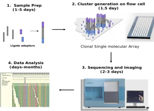
2.1.2.2 Illumina
The SOLEXA technique, Figure 7, acquired by Illumina in 2006 for over 600 M$ (www.illumina.com), consists of a proprietary flow cell surface for the parallel sequen-cing of DNA fragments (http://seqanswers.com/forums/showthread.php?t=21). Illu-mina reads are much shorter than 454 reads but their cost per base is significantly lower and their functional performance is higher. DNA is first fragmented, then it is
tached to adapters and denaturated in NaOH, then hybridization buffer is added to shift pH to neutral value and library is placed into the channel. In this way primer hybridize with a library molecule and the complementary strand have a chance to form a hybrid with an other primer. The fragments are then amplified locally and at each cycle the extended molecules bends and hybridizes to a second PCR primer forming a bridge. After more iterations the channel is characterized by clusters of oligonucleotides which are identical. At this point the system reads out the sequences of all clusters simultan-eously.
2.1.2.3 SOLiD
Sequencing by Oligonucleotide Ligation and Detection is a next-generation sequen-cing technology developed by Life Technologies (). This technique is based on “se-quencing ligation” of fluorochome-labeled oligonucleotides [13]. The DNA fragments hybridize to a specific section of the adapter. A set of four fluorescently labeled di-base probes compete for ligation to the sequencing primer. Specificity of the di-base probe is achieved by interrogating every 1st and 2nd base in each ligation reaction. Multiple cycles of ligation, detection and cleavage are performed with the number of cycles de-termining the eventual read length. Following a series of ligation cycles, the extension
product is removed and the template is reset with a primer complementary to the n-1 position for a second round of ligation cycles.
2.1.2.4 Third Generation Sequencing
It took nearly two decades to go from the release of the first semi-automated genome sequencer in the mid-1980s to the launch of Roche’s flagship 454 FLX next generation sequencer in 2005. The new wave of sequencers, (third generation sequencing) will likely enable scientists to reach the goal of the $US1000 human genome. But to do this, the cost of the sequencing chemistry needs to drop to around $US0.0000005/base,
or two millionths of a dollar per base (at a 10x coverage). Currently, the cheapest 2nd
generation sequencers cost about $US0.000001/base. And while this is a gigantic im-provement on 1985 prices when sequencing cost roughly $US10/base, we are still well short of the price target.
Third generation [14–16] of sequencing technology sees single molecules of DNA being sequenced without the need for cloning or PCR amplification and the inherent biases these procedures introduce. There are generally two types of detection methods for single molecule sequencing: those that rely on fluorescence and CCD capture, and those that don’t. Instruments that use the first of these detection methods include the Helicos Heliscope (http://www.helicosbio.com/Products/HelicosregGeneticAna-lysisSystem/HeliScopetradeSequencer/tabid/87/Default.aspx), launched in 2008; Pa-cific Biosciences single molecule real time sequencing (SMRT) machines (http://www.pacificbiosciences.com/products/smrt-technology/smrt-sequencing-ad-vantage), which have been shipped to their first customers; and Life Technologies-Vis-iGen system, which relies on fluorescence resonance energy transfer (FRET).
2.1.3 De Novo assembly algorithms 2.1.3.1 Introduction
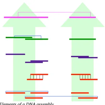
After DNA has been physically sheared into millions of reads, the assembler pieces together the many overlapping reads and reconstructs the original sequence. An as-sembled genome is usually composed of the following elements from simple to com-plex see Figure 8):
1. reads: the raw initial data
3. contigs: merging of overlapping unitgs plus consesus sequence; uses read pair-ing
4. scaffolds: linear sequence of contigs joined by mate pairs; uses read pairing
These elements are generated using data abstraction structures called graphs. The two most important graph type in current assembly packages are the overlap graph and the De Brujin graph; use of either of them actually characterize the two main assembly al-gorithms i.e. Overlap-Layout-Consesus (OLC) and De Brujin graph approach [17– 19].
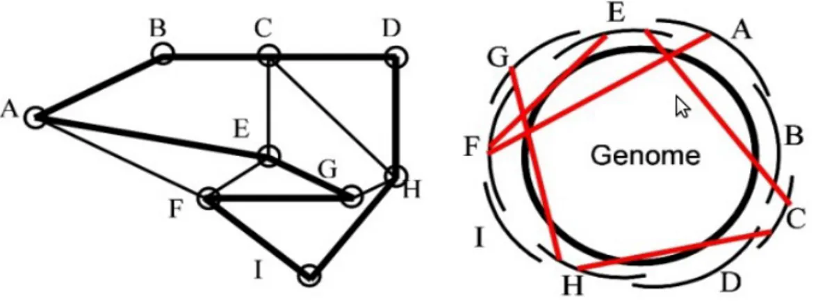
2.1.3.2 The OverlapLayoutConsesus approach
This approach consist of computing all pair-wise overlaps between each reads and col-lects information into the overlap graph. Each node represents a read and an edge de-notes an overlap between two reads. The overlap graph is used to compute a layout of reads and a consensus sequence of contigs. This method works best when there is a limited number of reads with significant overlap. A limit of this approach is that for the assembly of a simple organism the number of reads is very high (millions) and con-sequently the overlap graph became much large.
The OLC approach was typical of the Sanger-data assemblers. It was optimized for large genomes in software including Celera Assembler [8], Arachne [20], and CAP and PCAP [21]. OLC assemblers have three phases[22]:
1. Overlap discovery involves all-against-all, pair-wise read comparison.
2. Construction and manipulation of an overlap graph leads to an approximate read layout. The overlap graph need actual sequences, so large-genome graphs may fit into practical amounts of computer memory.
3. Multiple sequence alignment (MSA) determines the precise layout and then the consensus sequence. There is no known efficient method to compute the op-timal MSA [23]. Therefore, the consensus phase uses progressive pair-wise alignments guided by, for instance, the approximate read layout. Sequences must be loaded in RAM but computations may be partitioned by contig.
The Celera Assembler is a Sanger-era OLC assembler revised for 454 data [24]. The revised pipeline, called CABOG, discovers overlaps using compressed seeds. CABOG reduces homopolymer runs, that is, repeats of single letters, to single bases to over-come homopolymer run length uncertainty in data. CABOG builds initial unitigs ex-cluding reads that are substrings of other reads. Substrings account for a large portion of the data in high-coverage 454 data due to highly variable read lengths. CABOG avoids the substring-reads initially because they are more susceptible to repeat-induced false overlaps.
2.1.3.3 The De Brujin graph approach
De Brujin Graph (DBG) [25] can greatly reduce the computing resources necessary to assembly of a large number of reads by breaking reads into
smaller sequences of DNA, called k-mers (k parameter indicates the length of these small DNA sequences). This method permits to collect overlap information between the mers created rather than the reads. When two k-mers overlap by k-1 length, there is a directed edge from the first k-mer to the succeeding k-mer with a correesponding edge in the reverse direction. Multiple edges are derived if one k-mer overlaps with multiple, different k-mers by k-1 length on the side. A k-mer is considered to differ only in orientation with its reverse complement, and only one of the two is saved. Assembly packages based on the DBG include Velvet, Euler, Abyss and SOAP-denovo [26–28].
Four factors complicate the application of K-mer graphs to DNA sequence assembly: 1. DNA is double stranded. The forward sequence of any given read may overlap
the forward or reverse complement sequence of other reads and several differ-ent implemdiffer-entations of the DBG have proposed to address this problem.
2. Real genomes present complex repeat structures including tandem repeats, in-verted repeats, imperfect repeats, and repeats inserted within repeats. Repeats longer than K lead to tangled K-mer graphs that complicate the assembly prob-lem.
3. A palindrome is a DNA sequence that is its own reverse complement. Palin-dromes induce paths that fold back on themselves.
4. Real data includes sequencing error. DBG assemblers use several techniques to reduce sensitivity to this problem. First, they pre-process the reads to remove
Figure 10: Schematic diagram of the de Bruijn graph implementation
them, and then “erode” the lightly supported paths. Third, they convert paths to sequences and use sequence alignment algorithms to collapse nearly identical paths.
2.1.3.4 The MSRCA assembler
To overcome the limits of both OLC and the De Brujin approaches Zimin et al. (Zimin
et al., unpublished data) proposed a method that uses the De Brujin graph to merge 2nd
generation reads into longer reads (Super-Reads) and thus obtain a lossless data set di-mension shrinkage making it possible to apply the OLC method. Super-Reads are cre-ated mapping reads on the De Brujin graph and then merging them when a unique path is detected between k-mers thus yielding (almost) zero information loss. The MSR-CA assembler pipeline is composed of three main steps (see Figure 12) which corresponds to the three main software components:
1. K-mer counting performed with the Jellyfish package
2. Error-correction and Super-Reads creation using the De Brujin Graph; this is performed with software developed by Zimin et al.
3. Genome assembly using Super-Reads performed with a modified version of the OLC CABOG Assembler
Jellyfish generates k-mer counting statistics and is highly memory intensive; a
mam-malian data with 1-2*109 reads may require 256GB of RAM memory. Error-correction
attempts to remove sequencing errors using k-mer frequency; when correction is not possible reads are trimmed or completely discarded. Corrected reads generate much less improper branching in the graph and lead to better assembly results. Super-Reads have been covered above and CABOG is the modified version of the Celera assembler
able to work with 2nd generation data.
The basic goal if MSR-CA to reduce the complexity of the overlap-based assembly by transforming the high coverage (>50x) of the short reads into 5-6x coverage by su-per-reads, while making only the “easy” assembly decisions. This is done by creating A DBG is built using the most abundant data available (usually Illumina short paired ends) and then counting how many times each k-mer occurs in our reads. Each k-mer may be extended either by a A,C,G, or T (see Figure 11). If only one of these four oc-curs in the table, we say it has a unique following (or preceding) k-mer (such a k-mer is a simple k-mer). Examining the two simple (if any) k-mers at the ends of a read the read is extended by one base, using the uniquely occurring extension. Now the
exten-ded read has a new mer on its end. The process is repeated on each end until the k-mers on the end are no longer simple. The process stops at either end when the exten-sion is not unique of if there is indeed no extenexten-sion. The resulting read is defined as a Super-read. The two most important properties of the Super-reads are:
1. by design they are at least as long as the original reads
2. many of the original reads yield the same super-read. Using super-reads leads to vastly reduced data set
This much smaller data set is then assembled with a OLC assembler.
Figure 12: An example of a read whose super read has two k-unitigs
Read R contains k-mers M1 and M2 on its ends. M1 and M2 each belong to one and only one k-unitig K1 and K2. K-unitigs K1 and K2 are shown in blue and the matching k-mers M1 and M2 are shown in red and green respectively. K1 and K2 overlap by k-1 bases. We extend read R on both ends producing the super-read also depicted in blue. A super-read can consist of one k-unitig or can contain many k-unitigs.
2.2 SNP panels 2.2.1 Introduction
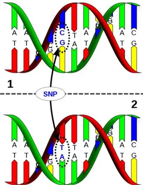
Single Nucleotide Polymorphisms (SNPs) are the most common form of genetic vari-ation between individuals, SNPs occur approximately once every 1,000 bases in mam-malians. SNPs are DNA sequence variations that occur when a single nucleotide (A,T,C, or G) in the genome sequence is altered (see Figure 13). Millions of these vari-ants are indexed in the National Center for Biotechnology Information's dbSNP data-base (http://www.ncbi.nlm.nih.gov/projects/SNP/), covering several organisms. To be classified as a SNP a variation's Minimum Allele Frequency (MAF) must be more than 1% (i.e. the rare variant needs to be present in at least 1% of the studied population) and must be inherited. On the other hand if the variation arises in a given generation or is less common is called a mutation.
SNP arrays (http://en.wikipedia.org/wiki/SNP_array) are a type of DNA microarrays used to to detect polymorphisms within a population comparing the studied sample with a reference genome and are thus species-specific. Microarray technology is well suited to SNP detection. Each SNP allele can be encoded in a single 25-base (or
base) oligonucleotide, and genotypes can be assigned with extremely high accuracy (99.8%; [29]) by detection of hybridization differences in genomic DNA (heterozy-gotes and homozy(heterozy-gotes can also be identified). Large numbers of SNP-specific oligo-nucleotides can be placed on a single chip and assayed in parallel on a single DNA sample, so the overall cost per genotype becomes very low. This technology allows a set of samples to be profiled for SNPs that cover the entire genome at high resolution, a "whole-genome association study." There are approximately 10 million SNPs across the worldwide human population, and over 5 million of these have sequences available in dbSNP at the NCBI Website (www.ncbi. nlm.nih.gov/SNP/snpsummary.cgi). Affy-metrix currently produces arrays of 10,000, 100,000, 500,000, and 1 million human SNPs. Using a different technology, Illumina offers a HumanHap300-Duo Genotyping BeadChip that contains a total of about 1 million tag SNPs from the HapMap Project. SNPs used to study other species such as cattle or sheep are usually less dense and
contain ~105 although more dense panels are being developed for species of economic
importance.
2.2.2 The Illumina BovineSNP50 chip
The BovineSNP50 v1 BeadChip (Figure 14) used in this work contains 54,001 SNPs
uniformly distributed across the cattle genome
(http://www.illumina.com/products/bovine_snp50_whole-genome_genotyping_kit-s.ilmn). It was developed by Illumina in collaboration with the USDA-ARS, Univer-sity of Missouri, and the UniverUniver-sity of Alberta. More than 24,000 SNP probes target novel SNP loci that were discovered by sequencing three pooled populations of eco-nomically important beef and dairy cattle using Illumina's Genome Analyzer. Addi-tional content was derived from publicly available sources such as the bovine refer-ence genome, Btau1, and the Bovine HapMap Consortium data set. The current ver-sion (v2) contains 54,609 SNPs. Recently, Illumina has presented the 777,000 SNP BovineHD BeadChip which expands the diversity of bovine breeds assessed in genetic prediction and enables more discoveries of quantitative traits.
2.3 Statistical methods
2.3.1 Infinitesimal model and Quantitative Trait Locus model (QTL)
The vast majority of economically important traits in livestock and aquaculture pro-duction systems are quantitative, that is they show continuous distributions. In at-tempting to explain the genetic variation observed in such traits, two models have been proposed, the infinitesimal model and the finite loci model. The infinitesimal model assumes that traits are determined by an infinite number of unlinked and additive loci, each with an infinitesimally small effect [30]. This model has been exceptionally valu-able for animal breeding, and forms the basis for breeding value estimation theory (e. g. [31]. However, the existence of a finite amount of genetically inherited material (the genome) and the revelation that there are perhaps a total of only around 20,000 genes or loci in the genome [32], means that there is must be some finite number of loci un-derlying the variation in quantitative traits. In fact there is increasing evidence that the distribution of the effect of these loci on quantitative traits is such that there are a few
Figure 15: Distribution of additive (QTL) effects from pig experiments
Distributions are scaled by the standard deviation of the relevant trait, and distribution of gene substitution (QTL) effects from dairy experiments scaled by the standard deviation of the relevant trait. B. Gamma Distribution of QTL effect from pig and dairy experiments, fitted with maximum likelihood.
genes with large effect, and a many of small effect ([33], [34]). In Figure 15, the size of quantitative trait loci (QTL) reported in QTL mapping experiments in both pigs and dairy cattle is shown. These histograms are not the true distribution of QTL effects however, they are only able to observe effects above a certain size determined by the amount of environmental noise, and the effects are estimated with error. In Figure 15A, the distribution of effects adjusted for both these factors is displayed. The distri-butions in Figure 15B indicate there are many genes of small effect, and few of large effect. The search for these loci, particularly those of moderate to large effect, and the use of this information to increase the accuracy of selecting genetically superior anim-als, has been the motivation for intensive research efforts in the last two decades. Two approaches have been used to uncover QTL. The candidate gene approach assumes that a gene involved in the physiology of the trait could harbour a mutation causing variation in that trait. The gene, or parts of the gene, are sequenced in a number of dif-ferent animals, and any variations in the DNA sequences, that are found, are tested for association with variation in the phenotypic trait. This approach has had some suc-cesses – for example a mutation was discovered in the oestrogen receptor locus (ESR) which results in increased litter size in pigs [35],[36] There are two problems with the candidate gene approach, however. Firstly, there are usually a large number of candid-ate genes affecting a trait, so many genes must be sequenced in several animals and many association studies so many genes must be sequenced in several animals and many association studies carried out in a large sample of animals (the likelihood that the mutation may occur in non-coding DNA further increases the amount of sequen-cing required and the cost). Secondly, the causative mutation may lie in a gene that would not have been regarded a priori as an obvious candidate for this particular trait. An alternative is the QTL mapping approach, in which chromosome regions associated with variation in phenotypic traits are identified. QTL mapping assumes the actual genes which affect a quantitative trait are not known. Instead, this approach uses neut-ral DNA markers and looks for associations between allele variation at the marker and variation in quantitative traits. A DNA marker is an identifiable physical location on a chromosome whose inheritance can be monitored. Markers can be expressed regions of DNA (genes) or more often some segment of DNA with no known coding function but whose pattern of inheritance can be determined. When DNA markers are available, they can be used to determine if variation at the molecular level (allelic variation at
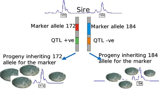
marker loci along the linkage map) is linked to variation in the quantitative trait. If this is the case, then the marker is linked to, or on the same chromosome as the investig-ated locus, a quantitative trait locus or QTL which has allelic variants causing vari-ation in the quantitative trait. Until recently, the number of DNA markers identified in livestock genome was comparatively limited, and the cost of genotyping the markers was high. This constrained experiments designed to detect QTL to using a linkage mapping approach. If a limited number of markers per chromosome are available, then the association between the markers and the QTL will persist only within families and only for a limited number of generations, due to recombination. For example in one sire, the A allele at a particular marker may be associated with the increasing allele of the QTL, while in another sire, the a allele at the same marker may be associated with the increasing allele at the QTL, due to historical recombination between the marker and the QTL in the ancestors of the two sires. To illustrate the principle of QTL map-ping exploiting linkage, consider an example where a particular sire has a large num-ber of progeny. The parent and the progeny are genotyped for a particular marker. At this marker, the sire carries the marker alleles 172 and 184, Figure 16. The progeny can then be sorted into two groups, those that receive allele 172 and those that receive allele 184 from the parent. If there is a significant difference between the two groups of progeny, then this is evidence that there is a QTL linked to that marker.
Figure 16: Linkage mapping
Principle of quantitative trait loci (QTL) detection, illustrated usingan abalone example. A sire is heterozygous for a marker locus, and carries the alleles 172 and 184 at this locus. The sire has a large number of progeny. The progeny are separated into two groups, those that receive allele 172 and those that receive allele 184. The significant difference in the trait of average size between the two groups of progeny indicates a QTL linked to the marker. In this case, the QTL allele increasing size is linked to the 172 allele and the QTL allele decreasing size is linked to the 184 allele.
QTL mapping exploiting linkage has been performed in all nearly livestock species for a huge range of traits [36]. The problem with mapping QTL exploiting linkage is that, unless a huge number of progeny per family or half sib family are used, the QTL are mapped to very large confidence intervals on the chromosome. To illustrate this, con-sider this formula [37] for estimating the 95% CI for QTL location for simple QTL mapping designs under the assumption of a high density genetic map:
CI=3000/(kNδ2)
CI =3000
k N δ2 (1)
where N is the number of individuals genotyped, δ allele substitution effect (the effect of getting an extra copy of the increasing QTL allele) in units of the residual standard deviation, k the number of informative parents per individual, which is equal 1 for half-sibs and backcross designs and 2 for F2 progeny, and 3000 is about the size of the cattle genome in centi-Morgans. For example, given a QTL segregates on a particular chromosome within a half sib family of 1000 individuals, for a QTL with an allele substitution effect of 0.5 residual standard deviations the 95% CI would be 12 cM. Such large confidence intervals have two problems. Firstly if the aim of the QTL map-ping experiment is to identify the mutation underlying the QTL effect, in a such a large interval there are a large number of genes to be investigated (80 on average with 20,000 genes and a genome of 3000 cM). Secondly, use of the QTL in marker assisted selection is complicated by the fact that the linkage between the markers and QTL is not sufficiently close to ensure that marker-QTL allele relationships persist across the population, rather marker-QTL phase within each family must be established to imple-ment marker assisted selection. An alternative, if dense markers were available, would be to exploit linkage disequilibrium (LD) to map QTL. Performing experiments to map QTL in genome wide scans using LD has recently become possible due to the availability of tenths of thousands of single nucleotide polymorphism (SNP markers) in cattle, pigs, chickens and sheep in the near future. A SNP marker is a difference in nucleotide between animals (or an animals pair of chromosomes), at a defined position in the genome, e. g.:
Animal 1. ACTCGGGC
Rapid developments in SNP genotyping technology now allow genotyping of a SNP marker in an individual for as little as 1c US.
2.3.2 Linkage Disequilibrium
The classical definition of linkage disequilibrium (LD) refers to the non-random asso-ciation of alleles between two loci. Consider two markers, A and B, that are on the same chromosome. A has alleles A1 and A2, and B has alleles B1 and B2. Four haplo-types of markers are possible A1_B1, A1_B2, A2_B1 and A2_B2. If the frequencies of alleles A1, A2, B1 and B2 in the population are all 0.5, then we would expect the fre-quencies of each of the four haplotypes in the population to be 0.25. Any deviation of the haplotype frequencies from 0.25 is linkage disequilibrium (LD), i.e. the genes are not in random association. As an aside, this definition serves to illustrate that the dis-tinction between linkage and linkage disequilibrium mapping is somewhat artificial – in fact linkage disequilibrium between a marker and a QTL is required if the QTL is to be detected in either sort of analysis. The difference is:
linkage analysis only considers the linkage disequilibrium that exists within families, which can extend for 10s of cM, and is broken down by recombina-tion after only a few generarecombina-tions
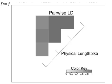
linkage disequilibrium (see Figure 17) mapping requires a marker to be in LD with a QTL across the entire population. To be a property of the whole popu-lation, the association must have persisted for a considerable number of gen-erations, so the marker(s) and QTL must therefore be closely linked.
D= freq ( A1B1)⋅freq( A2B2)− freq ( A1B2)⋅freq( A2B1) (2)
where freq (A1_B1) is the frequency of the A1_B1 haplotype in the population, and likewise for the other haplotypes. The D statistic is very dependent on the frequencies of the individual alleles, and so is not particularly useful for comparing the extent of LD among multiple pairs of loci (e. g. at different points along the genome). Hill and
Robertson [39] proposed a statistic, r2, which was less dependent on allele frequencies:
r2
=D /[ freq( A1) freq( B1) freq( A2) freq( B2)] (3)
where freq(A1) is the frequency of the A1 allele in the population, and likewise for the
other alleles in the population. Values of r2 range from 0, for a pair of loci with no
link-age disequilibrium between them, to 1 for a pair of loci in complete LD.
More precise estimates of LD are also tenable through fine mapping studies. Ulti-mately, through characterizing regions of high LD, mammalian genomes can be di-vided into LD blocks. These blocks are separated by hotspots, regions in which recom-bination events are more likely to occur [40]. An illustration of two LD blocks separ-ated by a recombination hotspot is given in Figure 3.2. In general, alleles tend to be more correlated within LD blocks than across LD blocks. Once regions of high LD are identified, investigators aim to determine the smallest subset of SNPs that character-izes the variability in this region, a process referred to as SNP tagging. Here the goal is to reduce redundancies in the genetic data. Consider a pair of SNPs that are in perfect
LD so that r2 is equal to 1. Genotyping both SNPs in this case is unnecessary since the
relationship between the two is deterministic. That is, by the definition of LD,
ledge of the genotype of one SNP completely defines the genotype of the second, and so there is no reason to sequence both loci. Well-defined tag SNPs will capture a sub-stantial majority of the genetic variability within an LD block.
When investigating cattle breeds, QTL effects have generally been related to poly-morphisms within functional candidate or other genes located in the QTL confidence interval. In an association study, a given SNP genotype may result associated to a phenotype if i) the SNP is the causative mutation; ii) the SNP is in high linkage dis-equilibrium with the gene under investigation; iii) the signal is a false positive (e.g. given by chance, by sampling bias due to a genetic sub-structure in the dataset, etc). For this reason only in a few cases causal mutations influencing milk traits have been identified using this approach; examples include K-casein ([41],[42]), SCD ([43],[44], DGAT1 ([45] and few others [46]. Even when there is a clear evidence of causality (e.g., DGAT1), genetic heterogeneity and genetic background may have a great impact on allele substitution effects [47]. Therefore, the potential application of gene/trait as-sociations in breeding must be tested on a breed by breed base and evaluated with at-tention and prudence.
2.3.3 Population genetics 2.3.3.1 Introduction
Population genetics [48] is the study of the frequency of occurrence of alleles within and between populations. Frequency information can be applied to a variety of popula-tion issues, including understanding the genetic basis of traits of interest, developing breeding strategies, and investigating the evolutionary history of populations. Tradi-tionally, the study of population genetics involved the identification of different alleles through observation of the expressed traits, broadly called the phenotype. Mendelian genetics allowed population geneticists to identify the heritable form of a gene (geno-type) including individual variants (alleles). Advances in molecular genetics facilitated identification of single genes at the molecular level. Regardless of the method used to identify genes and alleles, population geneticists use statistics of allele frequencies to understand and make predictions about gene flow in populations - past, present, and future.
It is often said that variation in genes is necessary to allow organisms to adapt to ever-changing environments. However, it is actually the variation in alleles that is critical. Alleles are different versions of the same gene that are expressed as different pheno-types. New alleles appear in a population by the random and natural process of muta-tion, and the frequency of occurrence of an allele changes regularly as a result of mutation, genetic drift, and selection. Nearly all mammals are diploid [49], i.e. they have two homologous copies of each chromosome and thus two copies (two alleles) of each gene, one inherited from each parent. If an individual has two different versions of a particular gene, the individual is said to be heterozygous for that gene; if the two alleles are the same, the individual is homozygous. Since a population needs variation, the measure of the amount of heterozygosity across all genes can be used as a general indicator of the amount of genetic variability and genetic health of a population.
Observed Heterozygosity (Ho) is the proportion of genes that are heterozygous
and the number of individuals that are heterozygous for each particular gene. For
a single gene locus with two alleles Ho is:
Ho=
nheterozygotes
Derivations of the above formula are used to calculate the HO when there are more
than two alleles for a particular locus, which is particularly common when microsatel-lite or simple sequence repeat (SSR) markers are applied for analysis of populations.
Expected Heterozygosity: The Expected Heterozygosity (He) is defined as the
es-timated fraction of all individuals that would be heterozygous for any randomly
chosen locus. The He differs from the Ho because it is a prediction based on the
known allele frequency from a sample of individuals.
Deviation of the observed from the expected can be used as an indicator of important population dynamics. Based on Mendelian genetics, it is possible to predict the prob-ability of the appearance of a particular allele in an offspring when the alleles of each parent are known. Similar predictions can be made about the frequencies of alleles in the next generation of an entire population. By comparing the predicted or "expected" frequencies with the actual or "observed" frequencies in a real population, one can in-fer a number of possible external factors that may be influencing the genetic structure of the population (such as inbreeding or selection).
2.3.3.2 Population structure
A population may be considered as a single unit. However, in many species and cir-cumstances, populations are subdivided in smaller units. Such subdivision may be the result of ecological (habitats are not continuous) or behavioural factors (conscious or unconscious relocation). If a population is subdivided, the genetic links among its parts may differ, depending on the real degree of gene flow taking place.
A population is considered structured if (1) genetic drift is occurring in some of its subpopulations, (2) migration does not happen uniformly throughout the population, or (3) mating is not random throughout the population. A population’s structure affects the extent of genetic variation and its patterns of distribution.
Here follows a little terminology in population genetics: ‘
Genetic drift’ refers to fluctuations in allele frequencies that occur by chance (particu-larly in small populations) as a result of random sampling among gametes. Drift de-creases diversity within a population because it tends to cause the loss of rare alleles, reducing the overall number of alleles.
‘Gene flow’ is the passage and establishment of genes typical of one population in the genepool of another by natural or artificial hybridization and backcrossing.
‘Non-random mating’ occurs when individuals that are more closely (inbreeding) or less closely related mate more often than would be expected by chance for the popula-tion. Self-pollination or inbreeding is similar to mating between relatives. It increases the homozygosity of a population and its effect is generalized for all alleles. Inbreed-ing per se does not change the allelic frequencies but, over time, it leads to homozy-gosity by slowly increasing the two homozygous classes.
‘Mutations’ could lead to occurrence of new alleles, which may be favourable or dele-terious to the individual’s ability to survive. If changes are advantageous, then the new alleles will tend to prevail by being selected in the population. The effect of selection on diversity may be: (i) ‘Directional’, where it decreases diversity; (ii) ‘Balancing’, where it increases diversity. Heterozygotes have the highest fitness, so selection fa-vours the maintenance of multiple alleles; and (iii) ‘Frequency dependent’, where it in-creases diversity. Fitness is a function of allele or genotype frequency and changes over time.
‘Migration’ implies not only the movement of individuals into new populations but that this movement introduces new alleles into the population (gene flow). Changes in gene frequencies will occur through migration either because more copies of an allele already present will be brought in or because a new allele arrives. The immediate ef-fect of migration is to increase a population’s genetic variability and, as such, helps in-crease the possibilities of that population to withstand environmental changes. Migra-tion also helps blend populaMigra-tions and prevent their divergence.
Hardy-Weinberg Principle: Based on Mendel's principles of inheritance, G.H. Hardy and Wilhelm Weinberg, independently developed the concept that is known today as the ‘Hardy-Weinberg Equilibrium’ or ‘Hardy-Weinberg Principle’ ([50], [51]), which states: "In a large, randomly breeding (diploid) population, allelic frequencies will re-main the same from generation to generation; assuming no unbalanced mutation, gene migration, selection or genetic drift." When a population meets all of the Hardy-Wein-berg conditions it is said to be in Hardy-WeinHardy-Wein-berg equilibrium. This equilibrium can be mathematically expressed based on simple binomial (for two alleles) or multinomial (multiple allele) distribution of the gene frequencies.
Testing for Hardy-Weinberg Equilibrium: Populations in their natural environment can never meet all of the conditions required to achieve Hardy-Weinberg equilibrium, thus their allele frequencies will change from one generation to the next and the population
will evolve. Just how far the population deviates from Hardy-Weinberg is an indication of the intensity of external factors, and can be determined by a statistical formula called a chi-square, which is used to compare observed versus expected outcomes. Effective Population Size: One of the many variables of population dynamics that can influence the rate and size of fluctuation in allele frequencies is population size. Ge-netic drift, the random increase or decrease of an allele's frequency, affects small popu-lations more severely than large ones, since alleles are drawn from a smaller parental gene pool. The rate of change in allele frequencies in a population is determined by the population's effective population size. The effective population size is the number of individuals that evenly contribute to the gene pool.
The actual number of individuals in a population is rarely the effective population size. This is because some individuals reproduce at a higher rate than others (have a higher fitness), the distribution of males and females may result in some individuals being un-able to secure a mate, or inbreeding reduces the unique contribution of an individual. The effective population size is a theoretical measure that compares a population's ge-netic behavior to the behavior of an "ideal" population. As the effective population size becomes smaller, the chance that allele frequencies will shift due to chance (drift) alone becomes greater.
Inbreeding and Relatedness: Small effective population size can result in a high occur-rence of inbreeding, or mating between close relatives. One of the effects of inbreeding is a decrease in the heterozygosity (increase in homozygosity) of the population as a whole, which means a decrease in the number of heterozygous genes in the individu-als. This effect places individuals and the population at a greater risk from homozyg-ous recessive diseases that result from inheriting a copy of the same recessive allele from both parents. The impact of accumulating deleterious homozygous traits is called ‘inbreeding depression’ - the loss in population vigour due to loss in genetic variability or genetic options.
2.3.3.3 F statistics
In the 1950s, Sewall Wright [52] developed a set of parameters called F statistics. If we assume that genotypes in the base population4 were in Hardy-Weinberg
propor-tions, then FIS is the probability that two alleles in an individual are identical by
des-cent (relative to the subpopulation from which they are drawn), FST is the probability
populations), and FIT is the probability that two alleles in an individual are identical by
descent (relative to the combined population). A random variable indicating whether or not two alleles are identical by descent takes on only two values, so these probabilities are equivalent to a correlation. The relationships among the F statistics can be deduced through the following:
FIT=1−
HI HT
1−FIT=(1−FIS)(1−FST)
(5)
where, HT = total gene diversity or expected heterozygosity in the total population as
estimated from the pooled allele frequencies, HI = intrapopulation gene diversity or
average observed heterozygosity in a group of populations, and HS = average expected
heterozygosity estimated from each subpopulation. F statistics estimate the deficiency
or excess of average heterozygotes in each population (FIS), the degree of gene
differ-entiation among populations in terms of allele frequencies (FST) and the the deficiency
or excess of average heterozygotes in a group of populations (FIT). There are two
sources of allele frequency difference among subpopulations in our sample:
(1) real differences in the allele frequencies among our sampled subpopulations and
(2) differences that arise because allele frequencies in our samples differ from those in the subpopulations from which they were taken.
Nei and Chesser [53] described the GST approach to account for the sampling error.
GST is an interpopulation differentiation measure when multiple loci are used for
ana-lysis. In other words, it measures the proportion of gene diversity that is measured among populations, when a large number of loci are sampled.
GST= DST HT HT=HS+DST DST=HT−HS (6)
where, DST is the interpopulation diversity, HT the total diversity and Hs the
2.3.4 Genomewide scan (GWAS) using SNP panels
The introduction of SNP chip technology, coupled with the success of the Interna-tional Haplotype Map (HapMap) Project (http://hapmap.ncbi.nlm.nih.gov), has led to an explosion of new research studies involving whole or partial genome-wide scans, commonly referred to as genome-wide association studies (GWAS). High-throughput SNP genotyping platforms, including Affymetrix and Illumina chips, provide for sim-ultaneous genotyping of 50,000 to one million SNPs. While a mammalian genome consists of approximately 3×10⁹ bases, variability in the genome may be captured by a subset of SNPs due to well-defined LD blocks and it has been proposed that whole genome-wide arrays of approximately one million SNPs are sufficient to characterize human genetic variability across a population. Several software tools have been de-veloped that apply these methods while accounting for the computational demands of whole genome-wide investigations: such as PLINK (http://pngu.mgh.harvard.edu/? purcell/plink/, [54]), SNPassoc (http://www.creal.cat/jrgonzalez/software.htm, [55])
and GenABEL (http://www.genabel.org, [56],[57]), haplostats (
http://cran.r-pro-ject.org/web/packages/haplo.stats/index.html). PLINK is a stand-alone software writ-ten in C++ (but it can handle in house writwrit-ten R plugins) while SNPassoc, haplostats and GenABEL are R packages available via CRAN (The Comprehensive R Archive Network, http://cran.r-project.org) and the latter has been extensively used in this work. The snpMatrix package is a component of the BioConductor open-source and open development software project for the analysis of genomic data [58]. GNU R is a free software language and environment for statistical computing and graphics (www.r-project.org).
2.3.4.1 Genotyping errors
A genotyping error is defined as a deviation between the true underlying genotype and the genotype that is observed through the application of a sequencing approach. These errors occur with varying degrees of frequency across the different technological platforms and arise for a variety of different reasons [59]. The most common statistical approach to identifying genotyping errors in population-based studies of unrelated in-dividuals is testing for a departure from HWE at each of the SNPs under investigation [60]. This proceeds using either an asymptotic χ2 -test or Fisher's exact test for associ-ation. There are a few notable drawbacks to this approach that we describe here, as
they are important to keep in mind in making the decision to remove SNPs from ana-lysis: using tests of HWE exclusively for identifying genotyping errors is that a depar-ture from HWE may in fact be a result of population substrucdepar-ture. Removing these SNPs from the analysis can therefore lead to a loss of data that are potentially inform-ative regarding underlying structure in our population and thus data preprocessing may become too stringent. Another drawback comes in disease studies deviations from HWE within individuals with disease (cases) can be due to association between geno-types and disease status for disease studies. In order to account for this possibility, some researchers advocate testing for departures from HWE only within the control population. This, however, can be misleading as well since removing cases from the analysis may lead to an apparent departure from HWE when indeed the entire popula-tion is in HWE. One resolupopula-tion to this problem for case-control studies involves ap-plication of a goodness-of-fit test to identify the most probable genetic disease model; e.g., dominant, recessive, additive or multiplicative [61]. This approach provides a means of distinguishing between departures from HWE that are due to the model for disease prevalence and those departures that are indeed a result of other phenomena, such as genotyping errors. Finally, multiplicity is also a challenge in this setting: mul-tiple testing leads to an inflation of the type-1 error rate. Therefore, if we test for a de-parture of HWE at each of multiple SNPs, then the likelihood of incorrectly rejecting the null hypothesis (and concluding HWD) can be substantial, particularly in the con-text of GWAS. This is attenuated to some extent by the correlated nature of the tests, arising from LD among SNPs; however, consideration of multiple testing adjustments is still warranted. In this setting, extreme thresholds for significance, such as 0.005 or 0.001, are common. If a departure from HWE is detected then the entire SNP is typic-ally removed from analysis: identification of specific records (individuals) within which an error exists are not provided by these approaches. Instead, it is assumed that the genotype information is incorrect across all individuals in the sample and the entire corresponding column is removed prior to statistical analysis.
2.3.4.2 Estimation of kinship matrix from dense SNP data
Kinship can be estimated from pedigree data using standard methods, for example the kinship for two outbred sibs is 1/4, for grandchild-grandparent is 1/8, etc. For an
-ations, pedigree information may be absent, incomplete, or not reliable. Moreover, the estimates obtained using pedigree data reflect the expectation of kinship, while the true realization of kinship may vary around this expectation. In presence of genomic data it
may therefore be desirable to estimate the kinship coe cient from these, and not fromffi
pedigree. It can be demonstrated that unbiased and positive semi-definite estimator of
the kinship matrix [62] can be obtained by computing the kinship coe cients betweenffi
individuals i and j with
̂ fij=1 L
∑
l =1 L (gi ,l−pl)(gj , l−pl) pl(1− pl) (7)where L is the number of loci, pl is the allelic frequency at l-th locus, gl,j is the
geno-type of j-th person at the l-th locus, coded as 0, 1/2, and 1, corresponding to the homo-zygous, heterohomo-zygous, and other type of homozygous genotype ([57],[62],[63]) The frequency is computed for the allele which, when homozygous, corresponds to the genotype coded as ”1’.
2.3.4.3 Analysis of structured populations
Populations may be structured in at least two ways. First, subjects may belong to
rather di erent genetic populations (e. g. humans from China and Africa) or they mayff
be sampled from a family in genetically isolated population. In the first case we need to consider that mean and variance of a trait under investigation may have different distributions (due maybe to environmental causes) while in the family based study en-vironmental influences are more or less uniform for all study participants but they are characterized by high and variable kinship between each other. These two types of
stratification may be expressed in terms of kinship: when we talk about di erent ”popff
-ulations”, we assume very low kinship and high genetic di erentiation between theff
members of these; when we talk about ”relatedness”, we assume high kinship and
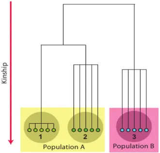
small degree of di erentiation. This is illustrated at ff Figure 19: if we expect that study
participants share common ancestors few (1-4) generation ago, the kinship between study participants is high, and the study can be classified as a family-based one (case); on the other hand, when common ancestors between study participants more remote the kinship between study participants is low, and such study may be classified as a population-based sample of ”independent” people (cases 2 and 3).
2.3.4.4 Genomic control
It follows that in presence of genetic structure standard association statistics may be
inflated and the distribution is described as λ · χ2; λ depends on the genetic structure of
the sample, as characterized by pairwise kinship, and sample size. For binary trait ana-lysis, it also depends on the composition of the case-control sample, as expressed by the proportion of cases/controls. For quantitative trait, it depends of heritability of the trait, and environmentally determined differences co-occuring with the difference in kinship. However, λ does not depend on the allele frequency. Therefore, for any
partic-ular study sample, if FST is constant over the genome, λ is also a constant. Therefore λ
can be estimated from the genomic data, using ”null” loci – a set of random markers, which are believed not to be associated with the trait. This estimate can then be used to correct the values of the test statistic at the tested loci – a procedure, known as ”gen-omic control”. The test statistics computed from these loci thus estimates the distribu-tion of the test statistic under the null hypothesis of no associadistribu-tion. Let us consider M
”null” markers, and denote the test statistic obtained from i-th marker as Ti2 . Given
ge-netic structure determines the inflation factor λ:T2∼λ⋅χ2 . The mean of a random
variable coming from χ12 is equal to 1; if a random variable comes from λ⋅χ2 ,
the mean would be λ. Thus we can estimate λ as the mean of the obtained ”null” tests.
Figure 19: Structured populations
Figure 6.5: Three samples from two populations. 1: Family-based sample; 2,3: random sample of ”independent” people
In practice, it is recommended to use the ratio between the observed median and the
one expected for χ12 :
̂λ= Median (Ti
2 )
0.4549 (8)
For the tested markers, the corrected value of the test statistic is obtained by simple
di-vision of the original test statistic value on λ: Tcorrected2 =Toriginal2 /λ . The genomic
control procedure is computationally extremely simple – one needs to compute the test statistic using a simple test (e.g. score test), compute the median to estimate λ, and di-vide the original test statistics values onto λ. How to choose ”null loci” is a GWA study? In a genome, we expect that a small proportion of markers is truly associated with the trait. Therefore in practice, all loci are used to estimate λ. Of cause, if very strong (or multiple weak) true associations are present, true association will increase the average value of the test, and genomic control correction will be conservative.
2.3.4.5 Analysis of family data
For pedigree-based data coming from genetically homogeneous population it can be shown that λ is a function of trait’s heritability and pedigree structure, expressed as kinship matrix. Thus, genomic control is a simple and valid method to study associ-ation in genetically homogeneous families. However, this method reduces all the abundant information about heritability and relationship into a single parameter λ, therefore it is not the most powerful method. In quantitative genetics, a mixed poly-genic model of inheritance may be considered as a valid alternative since it has sound theoretical bases and describes well inheritance of complex quantitative traits. It is
as-sumed that for each individual its ”individual” random residual ei is distributed as
Nor-mal with mean zero and variance σe. As these residuals are independent between
pedi-gree members, the joint distribution of residuals in the pedipedi-gree can be modelled using multivariate normal distribution with variance-covariance matrix proportional to the
identity matrix : e∼ MVN (0, I σe) . The model may expressed as:
Y =μ + G+ e (9)
trait values are equal to the sum of grand population mean, contribution from multiple
additively acting genes of small effect G, and residual error ei. Under this assumption,
distribu-tion with number of dimensions equal to the number of phenotyped people, with the
expectation of the trait value for some individual i equal to E [ yi]=μ where μ is
grand population mean (intercept). The variance-covariance matrix is defined through
its elements Vij – covariance between the phenotypes of subjects i and j:
Vij=σe 2 + σG2if i= j 2⋅fij⋅σG 2 if i≠ j (10)
where σG2 is variance due genes, fij is kinship between persons i and j, and σe is the
residual variance. The proportion of variance explainable by the additive genetic
ef-fects, is termed (narrow-sense) ”heritability”, h2:
h2 =σG
2
σe (11)
Fixed effects of some factor, e.g. SNP, may be included into the model by modifying the expression for the expectation, e.g. :
E [ yi]=μ+ βGg (12)
leading to so-called ”measured genotypes” model [64]. In essence, this is a linear mixed effects model – the one containing both fixed (e.g. SNP) and random (poly-genic) effects. A large body of literature is dedicated to this class of models, and find-ing the solution for such regressionrepresents no great methodological challenge. Ap-plicability of this model to GWA analysis was first proposed by Yu and colleagues [65].
2.3.4.6 The FASTA method
The polygenic component G in the mixed model approach describes the contribution
from multiple independently segregating genes all having a small additive e ect ontoff
the trait (infinitesimal model). For a subject for whom parents are unknown, it is
as-sumed that Gi is distributed as Normal with mean zero and variance σG. Assuming a
model of infinitely large number of genes, it can be shown that given polygenic values
for parents, the distribution of polygenic effects in o spring follows Normal distribuff
-tion with mean (Gm+Gf)/2 and variance σG/2, where Gm and Gf are the maternal
paternal polygenic values. From this, it can be shown that jointly the distribution of polygenic component in a pedigree can be described as multivariate normal with vari-ance-covariance matrix proportional to the relationship matrix Φ: