DIPARTIMENTO DI SCIENZE PURE E APPLICATE (DISPEA)
CORSO DI DOTTORATO DI RICERCA IN SCIENZE DI BASE E APPLICAZIONI
Curriculum Scienze della Terra
XXXI Ciclo
__________________________________________________________________
The role of orbital forcing in the early-middle Eocene
carbon cycle: a marine perspective
Il ruolo della forzante orbitale nel ciclo del carbonio dell’Eocene
inferiore-medio: una prospettiva marina
SSD Geo/01
RELATORE
DOTTORANDA
Chiar.mo Prof. Simone Galeotti
Dott.ssa Federica Francescone
__________________________________________________________________
ANNO ACCADEMICO 2017/2018
CONTENTS
INTRODUCTION ... 5
The early-middle Eocene and hyperthermal events ... 6
Astronomical Time Scale (ATS) ... 9
Outline of the Chapters ... 11
INTRODUZIONE ... 12
L'Eocene medio-inferiore e gli eventi ipertermici ... 13
La Scala Temporale Astronomica ... 15
Sommario ... 16
Chapter I: CYCLOCHRONOLOGY OF THE EARLY EOCENE CARBON ISOTOPE RECORD FROM A COMPOSITE CONTESSA ROAD-BOTTACCIONE SECTION (GUBBIO, CENTRAL ITALY) ... 18
ABSTRACT: ... 18
1.1 INTRODUCTION ... 18
1.2 MATERIAL AND METHODS ... 19
1.2.1 The Contessa Road-Bottaccione composite section ... 19
1.2.2 Magnetostratigraphy ... 21 1.2.3 Geochemistry ... 22 1.2.4 Spectral analysis ... 22 1.3 RESULTS ... 22 1.3.1 Magnetostratigraphy ... 22 1.3.2 Geochemical records ... 23 1.3.3 Spectral analysis ... 24 1.4 DISCUSSION ... 26
1.4.1 Cyclochronology of the CR-BTT composite section ... 26
1.4.2 Correlation with ODP Site 1258 and ODP Site 1263 ... 26
1.4.3 Implications for the astrochronological interpretation of the early Eocene ... 30
1.4.4 Orbital forcing, dissolution cycles and the EECO ... 33
1.5 CONCLUSIONS ... 34
Chapter II: A 9 MILLION-YEAR-LONG ASTROCHRONOLOGICAL RECORD OF THE EARLY-MIDDLE EOCENE CORROBORATED BY SEAFLOOR SPREADING RATES ... 36
ABSTRACT ... 36
2.1 INTRODUCTION ... 36
2.2 GEOLOGICAL SETTING ... 38
2.2.2 The Bottaccione Section ... 38
2.2.3 The Smirra Core ... 39
2.3.1 Magnetostratigraphy ... 39
2.3.2 Geochemistry and Physical Properties ... 40
2.3.2.1 Bottaccione Section ... 40
2.3.2.2 Smirra 1 Core ... 40
2.3.3 Spectral Analysis ... 40
2.3.4 Seafloor Spreading Rates ... 41
2.3.5 Comparison of synthetic and observed magnetic profiles ... 42
2.4 RESULTS ... 43 2.4.1 Bottaccione Section ... 43 2.4.1.1 Magnetostratigraphy ... 43 2.4.1.2 Geochemistry ... 43 2.4.2 Smirra 1 Core ... 44 2.4.2.1 Paleomagnetism ... 44
2.4.2.2 Bulk δ13C and Magnetic Susceptibility Records ... 45
2.5 GEOCHEMICAL CORRELATION OF THE UMBRIA-MARCHE RECORDS WITH ODP SITE 1258 AND ODP SITE 1263 ... 45
2.6 CYCLOSTRATIGRAPHY ... 47
2.6.1 The Bottaccione Record ... 47
2.6.2 The Smirra 1 Core Record ... 49
2.7 ASTROCHRONOLOGY AND THE UMBRIA-MARCHE AGE MODEL ... 52
2.7.1 C22r-C21r Magnetochron Interval ... 52
2.7.2 Seafloor Spreading Rates ... 55
2.8 DISCUSSION ... 59
2.9 CONCLUSIONS ... 65
Chapter III: STRATIGRAPHY OF EARLY TO MIDDLE EOCENE HYPERTHERMALS FROM POSSAGNO, SOUTHERN ALPS (ITALY) AND COMPARISON WITH GLOBAL CARBON ISOTOPE RECORDS ... 67
ABSTRACT ... 67
3.1 INTRODUCTION ... 67
3.2 MATERIAL AND METHODS ... 68
3.2.1 Geological setting ... 68 3.2.2 Geochemical Record ... 72 3.2.3 Spectral Analysis ... 73 3.2.4 Paleomagnetic analysis ... 73 3.3 RESULTS ... 74 3.3.1 Geochemical records ... 74
3.3.2 The Possagno composite stratigraphic record ... 74
3.4 CHEMOSTRATIGRAPHIC CORRELATION WITH ODP SITES 1258, 1263 AND THE UMBRIA-MARCHE BASIN ... 75
3.5.1 C24r-C24n stratigraphic interval ... 80
3.5.2 C23n-C22r stratigraphic interval ... 80
3.5.3 C22n-C21n stratigraphic interval ... 81
3.5.4. C22n stratigraphic interval in the Possagno Core B ... 82
3.6 DISCUSSION ... 82
3.6.1 Astrochronology ... 83
3.7 CONCLUSIONS ... 86
Chapter IV: DOES THE COMPARISON OF CARBON RELEASE AND INCREASE IN BOTTOM WATER TEMPERATURE ACROSS EARLY EOCENE HYPERTHERMALS PROVIDE A CASE FOR GREENHOUSE STATE CLIMATE SENSITIVITY? ... 87
ABSTRACT ... 87
4.1 INTRODUCTION ... 87
4.2 COVARIANCE OF δ13C AND δ18O ACROSS ETMs ... 88
4.3 THE PACIFIC AND ATLANTIC RECORDS ... 89
4.4 CONCLUSIONS ... 93
INTRODUCTION
In the last decades global concentration of atmospheric greenhouse gases (GHGs) have produced irreversible effects on our climate system (Intergovernmental Panel for Climate Change - IPCC - 2014). One issue of particular concern is the rising of the carbon dioxide (CO2) atmospheric concentration, which
overcame the threshold of 400 parts per million (ppm), modifying the terrestrial radiative forcing. Accordingly, the observed global mean surface temperature for the decade 2006-2015 was estimated to be on average 0.87°C higher than the average over the 1850-1900 period (IPCC, 2014).
The most recent IPCC report (2014) considers diverse future scenarios by the end of the 21th century,
characterized by different hypothesis of magnitude and emission rates of GHGs. These pathways, which have been defined as Representative Concentration Pathways (RCPs), include a stringent mitigation scenario (RCP2.6), two intermediate scenarios (RCP4.5 and RCP6.0) and one characterized by very high GHG concentration (RCP8.5). Scenarios without additional efforts to limit the emission lead to a RCP8.5 pathway (IPCC, 2014), which is characterized by atmospheric CO2 concentration of ~1000 ppm (Fig. 1).
Figure 1: Emissions of carbon dioxide (CO2) alone in the Representative Concentration Pathways (RCPs)
(lines) and the associated scenario categories used in Working Group (WG) III (colored areas show 5 to 95% range). The WGIII scenario categories summarize the wide range of emission scenarios published in the scientific literature and are defined on the basis of CO2-eq concentration levels (in ppm) in 2100 (IPCC,
2014).
Forecasting the magnitude of the global warming is one of the big scientific challenges. Indeed, all these pathways are characterized by a huge uncertainties due to the complexity of the climatic system.
Year Annual emissions (Gt CO 2 /yr) 1950 2000 2050 2100 −100 0 100 200 Historical emissions RCP2.6 RCP4.5 RCP6.0 RCP8.5
Full range of the WGIII AR5 scenario database in 2100 Annual anthropogenic CO2 emissions
>1000 720 −1000 580 −720 530 −580 480 −530 430 −480
WGIII scenario categories:
Moreover, the Climate Sensitivity, i.e. the response of the mean global surface temperature to a doubling of atmospheric CO2 concentration, which value is estimated between 1.5 and 4.5°C (IPCC, 2014), is
affected by a range of uncertainty as well. Longer-trend Climate Sensitivity is determined by internal feedbacks, both positive and negative, that either amplify or diminish the GHG effects as a response of the dynamic steady state variations.
Geological record can be used as a key that can lead to a better understanding of the impact of extreme global warming on the ocean-atmosphere coupled system and the relationship between carbon cycle and climate in worlds characterized by GHG concentrations very similar to that forecast by different RCP scenarios. Accordingly, certain time intervals in the past provide a unique opportunity to assess climate model because they capture the behavior of Earth’s climate system under pCO2 concentrations that likely
could be reached in the future. In particular, some time intervals and events are representative of mean global conditions similar to the more extreme scenarios predicted for the end of the century (RCP8.5), being characterized by levels equal or higher than 1000 ppm. The most recent geological time period characterized by this GHGs concentration is represented by the early Eocene and the so called hyperthermal events, occurring between ~56 and 51 million years ago (Ma).
The early-middle Eocene and hyperthermal events
The Cenozoic climate, the last ~65 million years (Myr), was characterized by a great variability (Fig. 2). As recorded in the d18O isotope curve, this time interval shows several steps at different time scales (107
-104 years), which can be associated with episodes of warming and cooling (Zachos et al., 2001). Most of
the variability is expressed through the Paleocene-Eocene epochs. A long-term global warming characterizes the evolving Greenhouse climate system through the late Paleocene and the early Eocene (~60-50 Ma), making the early Eocene (~56 to ~48 Ma) the warmest period over the entire Cenozoic. This gradual warming is followed by a long-term cooling eventually leading to the emplacement of a typical Icehouse climate system at the Eocene/Oligocene transition (~34 Ma) with the first significant appearance of a continental-scale Antarctic ice sheet (Zachos et al., 2008). The gradual warming that affected the Paleocene-early Eocene was punctuated by a series of transient (104-105 years) global warming events,
called hyperthermals (Cramer et al., 2003; Lourens et al., 2005; Galeotti et al., 2010, 2017; Zachos et al., 2010; Sexton et al., 2011; Littler et al., 2014; Kirtland Turner et al., 2014; Lauretano et al., 2015, 2016, 2018).
Figure 2: Global deep-sea oxygen and carbon isotope records based on data compiled from more than 40
DSDP and ODP sites (Zachos et al., 2001).
Hyperthermal events are linked to massive perturbations of the global carbon cycle related to the input of isotopically light carbon into the exogenic carbon pool (Dickens et al., 1995; Lourens et al., 2005; Zachos et al., 2005, 2010; Nicolo et al., 2007; Westerhold and Röhl, 2009; Galeotti et al., 2010; Galeotti et al., 2017). These extreme events are recorded globally as negative Carbon Isotopic Excursions (CIEs) and are associated with concomitant sediments depleted in calcium carbonate (CaCO3) in deep-sea and shallow
marine successions as a response to the sudden rising of the Carbonate Compensation Depth (CCD – Zachos et al., 2005) and the acceleration of the global hydrological cycle (Ravizza et al., 2001), thus runoff, respectively.
The most pronounced of these events is the Paleocene-Eocene Thermal Maximum (PETM), at ~56 Ma (Zachos et al. 2005; Tripati and Elderfield, 2005; Sluijs et al., 2008; Lourens et al., 2005; Westerhold et al., 2007; Galeotti et al., 2010, 2017). The PETM is characterized by the largest Cenozoic extinction of calcareous deep-marine benthic foraminifera (Thomas, 1989; Thomas and Shackleton, 1996) and is associated with a CIE of ~3‰ (Kennett and Stott, 1991; Koch et al., 1992; Thomas et al., 2002; Pagani et
al., 2006) and a negative excursion in d18O of benthic foraminifera of ~1.5‰ (Kennett and Stott, 1991;
Thomas and Shackleton, 1996; Zachos et al., 2001), which suggests an increase of ~6°C of sea-water temperature concomitant to the CIE. Beside the PETM, at least other two hyperthermal events, Eocene Thermal Maximum (ETM) 2 (also known as ELMO or H1) and ETM3 (also known as K or X event), at ~54.1 and ~52.8 Ma, respectively, occurred during the early Eocene (Lourens et al., 2005; Röhl et al., 2005). However, the associated CIEs are smaller (~2‰ and ~1‰ for ETM2 and ETM3, respectively) and also deep marine carbonate dissolution is less pronounced compared to the PETM (Lourens et al., 2005; Röhl et al., 2005).
Recently, similar events of comparable isotopic excursions have been discovered in the global bulk and benthic isotopic records (Sexton et al., 2011; Kirtland Turner et al., 2014; Lauretano et al., 2016, 2018; Westerhold et al., 2017, 2018). In particular, the Early Eocene Climatic Optimum (EECO), ~51 Ma, seems to be the maximal expression of these transient events. The EECO recorded the highest temperature of the Cenozoic (Zachos et al., 2001, 2008). During this time interval deep-water temperatures at high latitude were higher than present days, with peaks of 15-23°C (Zachos et al. 2010, Huber and Thomas 2008). Moreover, atmospheric pCO2 level was estimated at ~1000 ppm (Zachos et al., 2001). Based on the
available data (Hansen et al., 2008), the EECO is characterized by mean atmospheric CO2 levelswhich well
approach the RCP8.5 scenario. The interpretation of the EECO is an issue of particular interest because of its potential relevance for understanding the dynamics of this climatic system.
Although the hypothesis of successive releases of huge amounts of carbon as a mechanism for the emplacements of hyperthermals is widely accepted by the scientific community, a debate still exists on the possible sources. Various sources have been proposed, such as the destabilization of methane clathrates (Dickens et al., 1995), burning of terrestrial organic matter as extensive peat and coal deposits (Kurtz et al., 2003) and thawing and subsequent oxidation of the permafrost from the high latitude settings (DeConto et al., 2012). Several authors highlight the importance of the orbital forcing as a trigger mechanism for hyperthermal events (Westerhold and Röhl, 2009; Sexton et al., 2011; Kirtland Turner et al., 2014; Galeotti et al., 2010, 2017; Lauretano et al., 2016). Indeed, an astronomical forcing signature on the succession of hyperthermals allows to develop a cyclostratigraphy at a very high-resolution that permits to correlate each event to their respective counterparts of the Pacific and Atlantic Oceans, by designing a global observation system.
Furthermore, cyclostratigraphic approach permits to obtain an astronomical time scale which allows to verify the phase relationships between the orbital forcing and the sedimentary/geochemical response. The accuracy of the time scale is important for a better estimate of the emission rates of GHGs, in order to provides a crucial elements for the design of climate (paleo)models.
Moreover, the noted amplitude of the astronomical forcing allows to analyze the response of the system to a measurable forcing.
Astronomical Time Scale (ATS)
Determining an accurate age model of the carbon cycle aberrations is critical to explore causes and consequences of past climate change.
High-resolution CaCO3 and carbon isotope Cenozoic records show that the aberrations in the global
carbon cycle are paced by periodic oscillations in Earth’s astronomical parameters (Zachos et al., 2001; Cramer et al., 2003; Billups et al., 2004; Holbourn et al., 2005; Pälike et al., 2006), determined by Milankovitch cycles. These cyclical variations are mainly represented by the eccentricity long- and short- terms, obliquity and precession with characteristic period of ~400 and ~100, ~41 and ~20 kyr, respectively. Milankovitch cycles directly control the distribution of the Solar Energy on Earth and to a limited extent its total amount. The identification of these cyclic components in the terrestrial and marine sedimentary archives and the development of a cyclostratigraphic record tuned to the newest target curve (Laskar et al., 2011), provide a powerful astrochronological framework which can be used for the calibration of the entire Cenozoic timescale. In particular, the Earth’s orbital eccentricity component is widely used for astrochronological calibrations against the astronomical solution and the precision of the Astronomical Time Scale (ATS) strictly depends on the uncertainties in the eccentricity astronomical solution itself (Laskar et al., 2004, 2011). Indeed, Earth’s short eccentricity (~100 kyr) cycles are reliable back to ~50 Ma. Beyond this age, the chaotic behavior of large bodies within the asteroid belt makes it uncertain (Laskar et al., 2001, Westerhold et al., 2012). In spite of this, the long eccentricity (~400 kyr) cycle component is stable up to 200 Ma. The best approach for the development of a complete ATS for the early Cenozoic is the identification of the 400 kyr periodic component in the sedimentary archives, thus providing a powerful metronome for the cyclostratigraphic calibration of sedimentary archives and proxy record derived from them (Laskar et al., 2004; Hinnov and Hilgen, 2012).
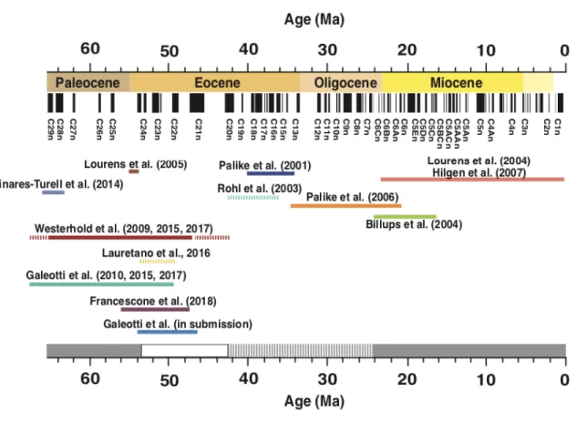
A cyclostratigraphic/astrochronologic numerical time scale is available for much of Cenozoic time interval (Pälike and Hilgen, 2008; Hinnov and Hilgen, 2012). However, uncertainties still affect the ATS, partly due to the scarcity of well-exposed and continuous geochemical and magnetostratigraphic records, in particular across the silica-rich (McGowran, 1989) EECO interval (Fig.3).
Figure 3: Summary of orbital timescale calibrations for the Cenozoic era in the context of climatic cycles
(Modified from Pälike and Hilgen, 2008). The lowermost horizontal gray line indicates a fairly stable and accurate astronomical age calibration with multiple site coverage (solid line), and more tentative or unverified age calibrations (dashed line). There is a significant gap in the middle Eocene, ~42 to 53 Myr ago (white box).
In this thesis we present a new high-resolution geochemical and bulk stable carbon isotopic record, integrated with bio- and magneto-stratigraphic analyses, from classic Tethyan successions cropping out in the Umbria-Marche basin (Italy) and from the Possagno section located in Southern Alps.
The main aim of this project was to contribute to the characterization of hyperthermal events across the early-middle Eocene time interval, defining a precise cyclochronological scheme of these events accompanied with the development of an accurate astronomically calibrated age model. It further can aid in closing the existing middle Eocene gap in the ATS (Pälike and Hilgen, 2008), partly due to the scarcity of well-exposed and continuous geochemical and magnetostratigraphic records across the silica-rich EECO interval (McGowran, 1989).
Outline of the Chapters
The early Eocene (~56 to ~48 Ma) is recorded in the pelagic Scaglia Rossa and Variegata Formations (Fms.) of the Umbria-Marche (U-M) Basin (central Italy). In Chapter I a high-resolution integrated magneto- chemo- and cyclo-stratigraphic record from two classic Tethyan section, Contessa Road and Bottaccione sections (Gubbio, Central Italy) is presented. The occurrence of a prominent, 10 cm-thick, marly layer laying ~2 m below the C23r-C23n magnetochron boundary has been used as a marker bed to correlate the two outcrops. This allows splicing a continuous high-resolution record spanning the lower part of magnetochron C24r to the upper part of magnetochron C22r. The detection of orbital components in the geochemical record allows establishing a relative cyclochronology of magnetochrons and hyperthermal events across the EECO, thus providing a criterion for its univocal identification in any cyclostratigraphic interpretation of marine successions. Moreover, cycle-counting across C23r and C23n magnetochrons allows solving the discrepancies between time scales based on astrochronological and radioisotopic age interpretation across what has been defined as “problematic interval” by Lauretano et al. (2016).
In Chapter II a new detailed integrated stratigraphy for the late early to middle Eocene from the Bottaccione section and a newly drilled core located at Smirra (central Italy) is presented. The new data, combined with the record previously published of Galeotti et al. (2017) from the same area, allowed us to extend it from the lower part of magnetochron C24n to the upper part of magnetochron C21n. The resulting record provides a continuous cyclochronological framework spanning 56.0 to 47.5 Ma. We independently test our age model by using sea-surface magnetic anomaly profiles from different oceanic basins, which provides evidence for the robustness of our astrochronological framework spanning the first 9 Myr of the Eocene. This work contributes to a better definition of the cyclochronology of hyperthermal events and to close the middle Eocene gap in the ATS. Indeed, this interval results to be well-preserved in the indurated limestone of the Umbria-Marche succession.
In Chapter III we present a high-resolution isotopic analysis of the early Eocene to middle Eocene (~51-45 Ma) time interval from the Possagno section located in the Southern Alps. The section provides a continuous and undisturbed chemostratigraphic and cyclochronological record across a critical time interval in terms of paleoceanographic and paleoclimatic evolution. Available deep-sea records provide a non-univocal astrochronological interpretation of the surveyed time interval as recently reported by different authors (Lauretano et al., 2016; Galeotti et al., 2017; Westerhold et al., 2017). The Possagno record, together with a core drilled in the same area, contributes to the definition of a correct interpretation of the astrochronology of the early-middle Eocene. Moreover, the good alignment, both on long- and short-trend terms, between Possagno carbon isotope record and coeval records, such as ODP Sites 1258, 1263, 1209 and the U-M basin, evidently results from factors of the carbon cycle which are reflected in the global record.
In Chapter IV the covariance between benthic carbon and oxygen stable isotopes during all major early Eocene hyperthermal events, i.e. ETM1 (or PETM), ETM2 ETM3), from South Atlantic (Leg 208, ODP Sites 1262, 1263 and 1265) and Pacific ocean records (ODP Site 1209 - Stap et al., 2010; Lauretano et al., 2015; Westerhold et al., 2018) has been presented. Regression line of stable d13C and d18O isotope
shifts during these events can be used to measure the global warming against the total amount of carbon release, which, in turn, should provide insights on the Climate Sensitivity during the Eocene. Several authors suggest that similar regression slopes in benthic foraminiferal records were caused by carbon release from the same source (Lauretano et al., 2015; Westerhold et al., 2018). In the light of evolving mean background conditions though the early Eocene, we rather point to a gradual depletion in the mass of the isotopically lighter reservoir, implying the existence of more than one reservoir.
INTRODUZIONE
Negli ultimi decenni la concentrazione globale di gas serra ha causato effetti irreversibili sul nostro sistema climatico (Intergovernmental Panel for Climate Change - IPCC - 2014). Una questione di particolare interesse è l'aumento della concentrazione atmosferica di anidride carbonica (CO2) che ha superato la soglia
di 400 parti per milione (ppm), modificando il bilancio radiativo terrestre. Di conseguenza, la temperatura superficiale media globale osservata per il decennio 2006-2015 è stata stimata essere mediamente 0.87°C superiore rispetto alla temperatura media nel periodo 1850-1900 (IPCC, 2014).
Il più recente report dell'IPCC (2014) contempla diversi scenari climatici futuri entro la fine del XXI secolo, caratterizzati da differenti ipotesi di tassi di emissione dei gas ad effetto serra. Questi modelli, definiti come Representative Concentration Pathways (RCP), includono uno scenario di attenuazione rigoroso (RCP2.6), due scenari intermedi (RCP4.5 e RCP6.0) e uno caratterizzato da una concentrazione di GHG molto alta (RCP8.5). In assenza di ulteriori sforzi per limitare le emissioni, lo scenario più probabile è l’RCP8.5 (IPCC, 2014), caratterizzato da una concentrazione di CO2 atmosferica di ~1000 ppm (Fig.1).
Prevedere la grandezza e il riscaldamento globale è una delle più grandi sfide scientifiche. Infatti, tutti questi modelli sono caratterizzati da enormi incertezze legate alla complessità del sistema climatico. Inoltre, la Sensibilità Climatica, ossia la risposta della temperatura media superficiale globale al raddoppio della concentrazione di CO2 atmosferica, il cui valore stimato risulta essere compreso tra 1.5 e 4.5°C (IPCC,
2014), è caratterizzata da una grande incertezza. La Sensibilità Climatica sul lungo termine è determinata dalla presenza di meccanismi di feedback interni, sia positivi che negativi, che amplificano o diminuiscono gli effetti dei gas ad effetto serra come risposta alle variazioni dinamiche dello stato di equilibrio.
Il record geologico può fornire importanti informazioni sull’'impatto del riscaldamento globale nel sistema accoppiato oceano-atmosfera e sulla relazione tra ciclo del carbonio e clima in mondi caratterizzati da concentrazioni di gas ad effetto serra molto simili a quelle previste dai diversi scenari RCP. Di conseguenza, alcuni intervalli temporali verificatisi in passato forniscono un'opportunità unica per valutare
il modello climatico poiché catturano il comportamento del sistema climatico della Terra in condizioni di concentrazioni di pCO2 che potrebbero essere raggiunte in futuro. In particolare, alcuni intervalli di tempo
ed eventi sono rappresentativi delle condizioni globali medie simili agli scenari più estremi previsti per la fine del secolo (RCP8.5), essendo caratterizzati da livelli uguali o superiori a 1000 ppm. Il periodo geologico più recente caratterizzato da questa concentrazione di gas serra è rappresentato dall’Eocene medio e dai cosiddetti eventi ipertermici, datati tra ~56 e 51 milioni di anni fa (Ma).
L'Eocene medio-inferiore e gli eventi ipertermici
Il clima nel Cenozoico (gli ultimi ~65 milioni di anni - Myr), è stato caratterizzato da una grande variabilità (Fig.2). Come registrato nella curva isotopica d18O, questo intervallo temporale mostra delle importanti
variazioni che si registrano a diverse scale temporali (107-104 anni) e che possono essere associate a episodi
di riscaldamento e raffreddamento (Zachos et al., 2001). La maggior parte della variabilità è espressa attraverso il Paleocene-Eocene. Un riscaldamento globale a lungo termine caratterizza l'evoluzione del sistema climatico di tipo Greenhouse attraverso il Paleocene superiore e l’Eocene inferiore (~60-50 Ma), rendendo l’Eocene inferiore (~56-48 Ma) il periodo più caldo dell'intero Cenozoico. Questo graduale riscaldamento è seguito da un raffreddamento a lungo termine che porta alla collocazione tipica di un sistema climatico di tipo Icehouse alla transizione Eocene/Oligocene (~34 Ma), con la prima comparsa significativa di una calotta polare antartica su scala continentale (Zachos et al., 2008). Il graduale riscaldamento che ha caratterizzato il Paleocene superiore-Eocene inferiore è stato punteggiato da una serie di eventi transienti (104-105 anni) di riscaldamento globale, chiamati eventi ipertermici (Cramer et al., 2003;
Lourens et al., 2005; Galeotti et al., 2010 , 2017; Zachos et al., 2010; Sexton et al., 2011; Littler et al., 2014; Kirtland Turner et al., 2014; Lauretano et al., 2015, 2016, 2018).
Gli eventi ipertermici sono associati a grandi perturbazioni del ciclo globale del carbonio legate all'input di carbonio isotopicamente leggero nel sistema accoppiato oceano/atmosfera (Dickens et al., 1995; Lourens et al., 2005; Zachos et al., 2005, 2010; Nicolo et al., 2007; Westerhold e Röhl, 2009; Galeotti et al., 2010; Galeotti et al., 2017). Questi eventi estremi sono registrati globalmente come escursioni negative nel record isotopico del carbonio (CIE) e sono associati a concomitanti sedimenti impoveriti nel contenuto di carbonato di calcio (CaCO3) nelle successioni marine profonde e superficiali, come risposta
all'innalzamento improvviso della profondità di compensazione del carbonato (CCD - Zachos et al., 2005) e all'accelerazione del ciclo idrologico globale (Ravizza et al., 2001), rispettivamente.
Il più pronunciato di questi eventi è il Paleocene-Eocene Thermal Maximum (PETM), a ~56 Ma (Zachos et al., 2005; Tripati and Elderfield, 2005; Sluijs et al., 2008; Lourens et al., 2005; Westerhold et al., 2007; Galeotti et al., 2010, 2017). Il PETM è caratterizzato dalla più grande estinzione cenozoica dei foraminiferi bentonici marini di origine calcarea (Thomas, 1989; Thomas and Shackleton, 1996) ed è associato ad una CIE di ~3 ‰ (Kennett and Stott, 1991; Koch et al., 1992; Thomas et al., 2002; Pagani et
al., 2006) e ad un'escursione negativa nel d18O dei foraminiferi bentonici di ~1.5‰ (Kennett and Stott,
1991; Thomas and Shackleton, 1996; Zachos et al. , 2001), suggerendo così un aumento di ~6°C delle temperature delle acque marine in concomitanza con la CIE. Oltre al PETM, almeno altri due eventi ipertermici, l’Eocene Thermal Maximum (ETM) 2 (noto anche come ELMO o H1) e l’ETM3 (noto anche come evento K o X), rispettivamente a ~54.1 e ~52.8 Ma, si sono verificati durante l’Eocene inferiore (Lourens et al., 2005; Röhl et al., 2005). Tuttavia, le CIE associate sono più piccole (~2‰ e ~1‰ per ETM2 e ETM3, rispettivamente), così come anche la dissoluzione del CaCO3 nei sedimenti marini è meno
pronunciata rispetto al PETM (Lourens et al., 2005; Röhl et al., 2005) .
Recentemente sono stati scoperti eventi analoghi nei record isotopici bulk e bentonici globali (Sexton et al., 2011; Kirtland Turner et al., 2014; Lauretano et al., 2016, 2018; Westerhold et al., 2017 , 2018). In particolare, l'Early Eocene Climatic Optimum (EECO), ~51 Ma, sembra essere la massima espressione di questi eventi transienti. L'EECO ha registrato la temperatura delle acque marine profonde più alta dell’intero Cenozoico (Zachos et al., 2011, 2008), raggiungendo picchi alle alte latitudini di 15-23°C (Zachos et al. 2010, Huber e Thomas 2008). Inoltre, i livelli di pCO2 atmosferici erano stimati a ~1000 ppm
(Zachos et al., 2001). Sulla base dei dati disponibili (Hansen et al., 2008), l’EECO è caratterizzato da valori medi di CO2 atmosferica che ben approssimano lo scenario RCP8.5. Lo studio dell’EECO risulta essere,
quindi, di particolare interesse grazie alla sua potenziale rilevanza nella comprensione delle dinamiche di tale sistema climatico.
Sebbene l'ipotesi di successivi rilasci di enormi quantità di carbonio come meccanismo determinante la messa in posto degli eventi ipertermici sia ampiamente accettato dalla comunità scientifica, le possibili fonti di carbonio sono ancora molto dibattute. Diverse sono le sorgenti di carbonio proposte, come la destabilizzazione dei metani idrati (Dickens et al., 1995), la combustione di materia organica terrestre derivante da vasti depositi di torba e carbone (Kurtz et al., 2003) e lo scioglimento e successiva ossidazione del permafrost dalle alte latitudine (DeConto et al., 2012). Diversi autori sottolineano l'importanza della forzante orbitale come meccanismo di innesco per gli eventi ipertermici (Westerhold e Röhl, 2009, Sexton et al., 2011; Kirtland Turner et al., 2014; Galeotti et al., 2010, 2017; Lauretano et al., 2016). Un controllo di tipo orbitale nelle successione di eventi ipertermici consente di sviluppare una ciclostratigrafia ad altissima risoluzione che permette di correlare ciascun evento alle rispettive controparti nell’Oceano Pacifico ed Atlantico, disegnando così un sistema di osservazione globale.
Inoltre, un approccio ciclostratigrafico permette di ottenere una scala temporale astronomica che consente di verificare i rapporti di fase tra la forzante orbitale e la risposta sedimentaria/geochimica. L’accuratezza della scala temporale è importante per una migliore stima dei tassi di emissione dei GHG, al fine di fornire elementi cruciali per la progettazione dei modelli (paleo)climatici.
Infine, avendo la forzante orbitale ampiezza nota, consente di studiare la risposta del sistema ad un forcing misurabile.
La Scala Temporale Astronomica
Determinare un modello di età accurato degli eventi di aberrazione del ciclo del carbonio è fondamentale per esplorare le cause e le conseguenze dei cambiamenti climatici del passato.
I records ad alta risoluzione del CaCO3 e degli isotopi del carbonio attraverso il Cenozoico mostrano
come le aberrazioni nel ciclo globale del carbonio siano controllate da oscillazioni periodiche nei parametri astronomici della Terra (Zachos et al., 2001; Cramer et al., 2003; Billups et al., 2004; Holbourn et al., 2005; Pälike et al., 2006), determinate dai cicli di Milankovitch. Queste variazioni cicliche sono rappresentate principalmente dall'eccentricità, a lungo e breve termine, obliquità e precessione, con periodi caratteristici di ~400 e ~100, ~41 e ~20 kyr, rispettivamente. I cicli di Milankovitch controllano direttamente la distribuzione dell'energia solare sulla Terra e, in misura limitata, la sua quantità totale. L'identificazione di queste componenti cicliche negli archivi sedimentari terrestri e marini e lo sviluppo di un record ciclostratigrafico sintonizzato alla nuova soluzione astronomica target (Laskar et al., 2011), forniscono un potente impianto astrocronologico che può essere utilizzato per la calibrazione della scala cronologica dell’intero Cenozoico. In particolare, la componente orbitale dell’eccentricità è ampiamente utilizzata per le calibrazioni astrocronologiche sintonizzate alla soluzione astronomica disponibile e la precisione della Scala Temporale Astronomica (ATS) dipende strettamente dalle incertezze nella soluzione astronomica della stessa eccentricità (Laskar et al., 2004, 2011). Infatti, i cicli di eccentricità breve della Terra (~100 kyr) sono affidabili fino a ~50 Ma. Oltre questa età, il comportamento caotico di grandi corpi all'interno della fascia degli asteroidi li rende incerti (Laskar et al., 2001; Westerhold et al., 2012). Nonostante ciò, la componente dei cicli di eccentricità a lungo termine (~400 kyr) è stabile fino a ~200 Ma. L'approccio migliore per lo sviluppo di una ATS completa per il Cenozoico inferiore consiste nell’identificazione della componente periodica dei 400 kyr negli archivi sedimentari, fornendo così un potente metronomo per la calibrazione ciclostratigrafica degli archivi sedimentari e dei proxy record derivati da essi (Laskar et al., 2004; Hinnov and Hilgen, 2012).
Una scala temporale ciclostratigrafica/astrocronologica è già disponibile per gran parte del Cenozoico (Pälike and Hilgen, 2008; Hinnov and Hilgen, 2012). Tuttavia, molte sono le incertezze che caratterizzano l'ATS, dovute alla scarsità di records geochimici e magnetostratigrafici continui e ben esposti soprattutto attraverso l’EECO (McGowran, 1989 - Fig.3).
In questa tesi viene presentato un nuovo record geochimico ad alta risoluzione dell’isotopo stabile del carbonio, integrato con analisi bio- e magneto-stratigrafiche, delle classiche successioni Tetidee che affiorano nel bacino Umbro-Marchigiano (Italia) e dalla sezione Possagno situata nelle Alpi del Sud.
Lo scopo principale di questo progetto è quello di contribuire alla caratterizzazione degli eventi ipertermici attraverso l’Eocene medio-inferiore, definendo un preciso schema ciclocronologico di questi eventi accompagnato dallo sviluppo di un accurato modello di età calibrato astronomicamente.
Inoltre, contribuisce alla chiusura del gap esistente nell’ATS in corrispondenza dell’Eocene medio (Pälike e Hilgen, 2008), dovuto in parte alla scarsità di records ben preservati e continui attraverso l’intervallo ricco di silice dell’EECO (McGowran, 1989).
Sommario
L’Eocene inferiore (~56 a ~48 Ma) è registrato nelle formazioni pelagiche della Scaglia Rossa e Variegata nel bacino Umbro-Marchigiano (Italia centrale). Nel Capitolo I è presentato un record integrato magneto- chemo- e ciclo-stratigrafico ad alta risoluzione di due classiche sezioni Tetidee, le sezioni della Contessa Road e del Bottaccione (Gubbio, Italia centrale). La presenza di un prominente strato marnoso di 10 cm di spessore situato a ~2 m sotto il limite del magnetochron C23r-C23 è utilizzato come marker di riferimento per correlare i due affioramenti. Ciò consente di creare un record continuo ad alta risoluzione che si estende dalla parte inferiore del magnetochron C24r alla parte superiore del magnetochron C22r. L’identificazione delle componenti orbitali nel record geochimico consente di stabilire una ciclocronologia flottante dei magnetochrons e degli eventi ipertermici attraverso l’EECO, fornendo così un criterio univoco per la sua identificazione in qualsiasi interpretazione ciclostratigrafica delle successioni marine. Inoltre, il conteggio dei cicli attraverso i magnetochons C23r e C23n consente di risolvere le discrepanze tra le scale temporali basate sull'interpretazione astrocronologica e sull'età radioisotopica attraverso quello che è stato definito "intervallo problematico" da Lauretano et al. (2016).
Nel Capitolo II è presentata una stratigrafia integrata dell'Eocene inferiore-medio della sezione Bottaccione e del nuovo record recuperato attraverso un carotaggio effettuato a Smirra (Italia centrale). I dati ottenuti sono stati combinati con il record precedentemente pubblicato da Galeotti et al. (2017) proveniente dalla stessa area, permettendoci così di estendere il record dalla parte inferiore del magnetochron C24n alla parte superiore del magnetochron C21n. Il record risultante fornisce un quadro ciclocronologico continuo che si estende da 56.0 a 47.5 Ma. Inoltre, il nostro modello temporale è testato in modo indipendente utilizzando i profili di anomalia magnetica della superficie del mare provenienti da diversi bacini oceanici, fornendo così una prova della robustezza del nostro inquadramento astrocronologico per i primi 9 Myr dell'Eocene. Questo lavoro contribuisce ad una migliore caratterizzazione della ciclocronologia degli eventi ipertermici e alla chiusura del gap attraverso l’Eocene medio nell’ATS. Infatti, questo intervallo è ben conservato nel calcare della successione Umbro-Marchigiana.
Nel Capitolo III presentiamo un'analisi isotopica ad alta risoluzione dell’intervallo compreso tra l’Eocene inferiore e medio (~51-45 Ma) dalla sezione di Possagno situata nelle Alpi meridionali. La sezione fornisce una record chemostratigrafico e ciclocronologico continuo ed indisturbato attraverso un intervallo temporale critico in termini di evoluzione paleoceanografica e paleoclimatica. I record delle acque profonde disponibili forniscono un'interpretazione astrocronologica non univoca dell'intervallo di tempo analizzato,
come recentemente riportato da diversi autori (Lauretano et al., 2016; Galeotti et al., 2017; Westerhold et al., 2017). Il record di Possagno, insieme ad un carota recuperata nella stessa area, contribuisce alla definizione di una corretta interpretazione astrocronologica dell'Eocene inferiore-medio. Inoltre, il buon allineamento, sia a lungo che a breve termine, tra il record isotopo del carbonio di Possagno e records coevi, come i Siti ODP 1258, 1263, 1209 e il bacino Umbro-Marchigiano, deriva da fattori del ciclo del carbonio che si riflettono nel a livello globale.
Nel Capitolo IV è stata presentata la covarianza tra gli isotopi stabili bentonici del carbonio e dell'ossigeno attraverso i principali eventi ipertermici dell'Eocene inferiore, ovvero per l’ ETM1 (o PETM), l’ETM2 e l’ETM3, provenienti dai records oceanici dell’Atlantico (Leg 208, ODP Sites 1262, 1263 e 1265) e del Pacifico (ODP Site 1209 - Stap et al., 2010; Lauretano et al., 2015; Westerhold et al., 2018). La linea di regressione del δ13C e del δ18O durante questi eventi può essere utilizzata per misurare il riscaldamento
globale rispetto alla quantità totale di carbonio rilasciata, che, a sua volta, dovrebbe fornire informazioni sulla Sensibilità Climatica durante l'Eocene. Diversi autori suggeriscono che pendenze di regressione simili nei records dei foraminiferi bentonici sono state causate dal rilascio di carbonio proveniente dalla stessa fonte (Lauretano et al., 2015; Westerhold et al., 2018). Alla luce dell'evoluzione delle condizioni di background attraverso l’Eocene inferiore, proponiamo piuttosto un progressivo esaurimento nella massa di carbonio proveniente dal reservoir isotopicamente più leggero, implicando l'esistenza di più di un reservoir.
Chapter I
CYCLOCHRONOLOGY OF THE EARLY EOCENE CARBON ISOTOPE
RECORD FROM A COMPOSITE CONTESSA ROAD-BOTTACCIONE
SECTION (GUBBIO, CENTRAL ITALY)
Galeotti Simone, Moretti Matteo, Sabatino Nadia, Sprovieri Mario, Ceccatelli Mattia, Francescone Federica, Lanci Luca, Lauretano Vittoria, Monechi Simonetta
Published on Newsletters on Stratigraphy, Vol. 50/3 (2017), 231–244, DOI: 10.1127/nos/2017/0347.
ABSTRACT: High-resolution geochemical time series from the composite Contessa Road-Bottaccione (CR-BTT) section (central Italy) allows testing the global significance of Early Eocene short- and long-term carbon isotope trends by comparison with available records from oceanic successions. Spectral analysis reveals Milankovitch frequency band fluctuations in the concentration of CaCO3. Extraction of the
short- and long- eccentricity orbital periodicities from the wt.% CaCO3 record provides a relative
cyclochronology for the interval spanning ~49.5 Ma to ~52.5 Ma corresponding to magnetochron C22r to the top of C24n thus extending the cyclochronology already available from the same section in the interval between ~52.0 to ~56 Ma, spanning the lower C24r to upper C23r. Recognition of orbitally forced sedimentary cycles, corresponding to the long (405 kyr) and short (100 kyr) eccentricity, allows to test the chemostratigraphic alignment with ODP Site 1258 and ODP Site 1263 records and to obtain a correlation of hyperthermal events to an unambiguous magnetostratigraphic record across the interval corresponding to the Early Eocene Climatic Optimum and to refine the astrochronological interpretation of the Ypresian Stage.
1.1 INTRODUCTION
The Early Eocene Climatic Optimum (EECO) recorded the highest mean global temperature of the last 65 millions of years (Myr) (Zachos et al., 2001, 2008). Geochemical and paleontological proxies indicate that high latitude temperatures were much higher than present day with peaks of 15–23°C (Zachos et al., 2010; Huber and Thomas, 2008). Deep-water temperatures were 10–12°C higher than present day, depressing the meridional gradient and the efficiency of global oceanic circulation (Zachos et al., 2001; Huber and Caballero, 2011). The extreme climate of the EECO represents a case study for the so-called super-greenhouse state under very high atmospheric CO2 concentrations (Pagani et al., 2005). According to Lunt
et al. (2011), the EECO is the maximal expression of a series of transient warming events called hyperthermals that punctuated the long-term warming trend starting in the middle Paleocene around 60
million years ago (Ma) and culminating at ~51 Ma. Hyperthermals are geologically brief (104–105 yr) events
characterised by large global temperature increase and negative carbon isotope excursions, caused by the release of massive amounts of isotopically light carbon into the exogenic pool (Zachos et. al., 2005; Lourens et al., 2005; Röhl et al., 2007; Agnini et al., 2007; Nicolo et al., 2009). It has been suggested that these events were triggered by orbital forcing (Cramer et al., 2003; Lourens et al., 2005; Galeotti et al., 2010; Littler et al., 2014; Lauretano et al., 2015). The most important hyperthermal events are represented by the Paleocene–Eocene Thermal Maximum (PETM) at ~56.1 Ma (Kennett and Stott, 1991; Koch et al., 1992; Nicolo et al., 2007; Zachos et al., 2005; Galeotti et al., 2010; DeConto et al., 2012), the Eocene Thermal Maximum 2 (ETM2), at ~54.1 Ma, and the ETM3 at ~52.8 Ma (Cramer et al., 2003; Lourens et al., 2005; Westerhold et al., 2007; Galeotti et al., 2010). Proposed carbon sources for the emplacement of these events on an orbital time scale include oceanic gas hydrates (Dickens et al., 1995), oceanic dissolved organic carbon (Sexton et al., 2011, Kirtland Turner et al., 2014) and permafrost (DeConto et al., 2012). According to Lunt et al. (2011) changing mean boundary conditions across the gradual warming that culminates at the EECO, resulted in diminished magnitude and increasing frequency of hyperthermal events, in response to the climate system getting closer to the threshold for carbon release and decreasing time for the recharging of the gas hydrate reservoir. The scarcity of well-preserved and continuous geochemical records across the early Eocene, particularly across the silica-rich EECO interval (McGowran, 1989) makes it difficult to obtain an observational basis to test this hypothesis. In fact, a univocal cyclostratigraphic interpretation across this interval (problematic interval of Lauretano et al., 2016) has proved to be a challenging task to achieve. Here we present an integrated magneto-, chemo- and cyclo- stratigraphic record from the Bottaccione-Contessa Road composite section, which provides an exceptionally well-preserved archive of orbital forcing signature across this critical interval.
1.2 MATERIAL AND METHODS
1.2.1 The Contessa Road-Bottaccione composite section
Outcrops in the Umbria–Marche Basin of central Italy provide a continuous record of the Paleocene and Early Eocene, which is locally preserved in the pelagic red limestones of the Scaglia Rossa Formation. Well-known early Cenozoic sections in the classic Gubbio area were used to develop magneto- and biostratigraphic relationships that enabled the first calibration of geomagnetic reversals for most of the Paleogene interval (Lowrie et al., 1982; Napoleone et al., 1983). Here we focus on two sections, Contessa Road (lat. 43°22 47 N; long. 12°33 50 E) and Bottaccione (lat. 43° 21 56 N; long. 12° 34 57 E - Fig. 1.1) to build a composite, stratigraphically continuous succession spanning the lower part of magnetochron C24r to the lower part of magnetochron C22r.
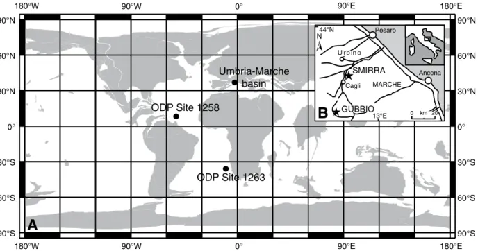
Figure 1.1: Paleogeographic reconstruction for the Early Eocene (51 Ma) showing the location of the three
sites discussed in text. Paleogeographic map is from the Ocean Drilling Stratigraphic Network Plate Tectonic Reconstruction Service: (http://www.odsn.de/odsn/ services/paleomap/paleomap.html).
The 54.5m-thick Contessa Road section starts at the Cretaceous-Paleogene (K/Pg) boundary, defined as level 0 in the measured section. Previous bio- and magnetostratigraphy of the lower Paleogene portion of the Contessa Road section, which is locally represented by the Scaglia Rossa limestones and marly limestones, have been published by Lowrie et al. (1982) and Galeotti et al. (2000, 2005) from ca. 24 m above the K/Pg boundary to the top of the section at 54.5 m above the K/Pg boundary. The integrated bio-, magneto- and chemostratigraphic analysis of the upper Paleocene to lower Eocene (Galeotti et al.bio-, 2010; Coccioni et al., 2012) reveals the occurrence of carbon isotope excursions (CIEs) associated to hyperthermal events as previously described from oceanic successions. A more detailed description of the lower Eocene Contessa Road is given by Galeotti et al. (2000, 2010). The outcrop is poorly exposed from the top of C23r magnetochron, which does not allow an accurate high-resolution sampling. In order to extend the high-resolution geochemical record already available for the Early Eocene at the Contessa Road section (Galeotti et al., 2010), we sampled the overlying stratigraphic interval in the nearby Bottaccione section. In particular, the record of Galeotti et al. (2010), spanning 31.3-47 m above the K/Pg boundary in the Contessa Road section, has been extended by sampling the interval spanning 47-54 m above the K/Pg in the Contessa Road record and 50.2-63.6 m above the K/Pg boundary in the Bottaccione section (see also Fig. 1.2). The lower–middle Eocene at Bottaccione has been previously studied for bio- and magnetostratigraphy by Napoleone et al. (1983). The studied interval is mainly calcareous although a series of marly layers, up to 10 cm-thick, occur, particularly in its lower part. Chert nodules and layers are also present although sparse.
2011). The extreme climate of the EECO represents a case study for the so-called super-greenhouse state un-der very high atmospheric CO2concentrations (Pagani et al. 2005). According to Lunt et al. (2011), the EECO is the maximal expression of a series of transient warm-ing events called hyperthermals that punctuated the longterm warming trend starting in the middle Paleo -cene around 60 million of years ago (Ma) and culmi-nating at ~51 Ma. Hyperthermals are geologically brief (104–105yr) events characterised by large global tem-perature increase and negative carbon isotope excur-sions, caused by the release of massive amounts of iso-topically light carbon into the exogenic pool (Zachos et. al. 2005, Lourens et al. 2005, Röhl et al. 2007, Agni-ni et al. 2007, Nicolo et al. 2009). It has been suggested that these events were triggered by orbital forcing (Cramer et al. 2003, Lourens et al. 2005, Galeotti et al. 2010, Littler et al. 2014, Lauretano et al. 2015). The most important hyperthermal events are represented by the Paleocene–Eocene Thermal Maximum (PETM) at ~56.1 Ma (Kennett and Stott 1991, Koch et al. 1992, Nicolo et al. 2007, Zachos et al. 2005, Galeotti et al. 2010, DeConto et al. 2012), the Eocene Thermal Maximum!2 (ETM2), at ~54.1 Ma, and the ETM3 at ~52.8 Ma (Cramer et al. 2003, Lourens et al. 2005, Westerhold et al. 2007, Galeotti et al. 2010). Proposed carbon sources for the emplacement of these events on an orbital time scale include oceanic gas hydrates (Dickens et al. 1995), oceanic dissolved organic carbon (Sexton et al. 2011, Kirtland Turner et al. 2014) and permafrost (DeConto et al. 2012). According to Lunt et al. (2011) changing mean boundary conditions across the gradual warming that culminates at the EECO, re-sulted in diminished magnitude and increasing fre-quency of hyperthermal events, in response to the cli-mate system getting closer to the threshold for carbon release and decreasing time for the recharging of the gas hydrate reservoir. The scarcity of well-preserved and continuous geochemical records across the Early
Eocene, particularly across the silica-rich EECO inter-val (McGowran 1989) makes it difficult to obtain an observational basis to test this hypothesis. In fact, a univocal cyclostratigraphic interpretation across this interval (problematic interval of Lauretano et al. 2016) has proved to be a challenging task to achieve. Here we present an integrated magneto, chemo and cyclo -stratigraphic record from the Bottaccione-Contessa Road composite section, which provides an exception-ally well-preserved archive of orbital forcing signature across this critical interval.
2. Material and methods
2.1 The Contessa Road-Bottaccione composite section
Outcrops in the Umbria–Marche Basin of central Italy provide a continuous record of the Paleocene and Early Eocene, which is locally preserved in the pelagic red limestones of the Scaglia Rossa Formation. Well-known early Cenozoic sections in the classic Gubbio area were used to develop magneto- and biostrati-graphic relationships that enabled the first calibration of geomagnetic reversals for most of the Paleogene interval (Lowrie et al. 1982, Napoleone et al. 1983). Here we focus on two sections, Contessa Road (lat. 43° 22! 47" N; long. 12° 33! 50" E) and Bottaccione (lat. 43° 21! 56" N; long. 12° 34! 57" E) (Fig. 1) to build a composite, stratigraphically continuous succession spanning the lower part of magnetochron C24r to the lower part of magnetochron C22r.
The 54.5 m-thick Contessa Road section starts at the Cretaceous-Paleogene (K/Pg) boundary, defined as level!0 in the measured section. Previous bio- and mag-netostratigraphy of the lower Paleogene portion of the Contessa Road section, which is locally represented by the Scaglia Rossa limestones and marly limestones,
Simone Galeotti et al. 232
Fig. 1. Paleogeographic reconstruction for the Early Eocene (51 Ma) showing the loca-tion of the three sites discussed in text. Paleo-geographic map is from the Ocean Drilling Stratigraphic Network Plate Tectonic Recon-struction Service: (http://www.odsn.de/odsn/ services/paleomap/paleomap.html).
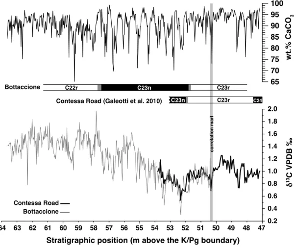
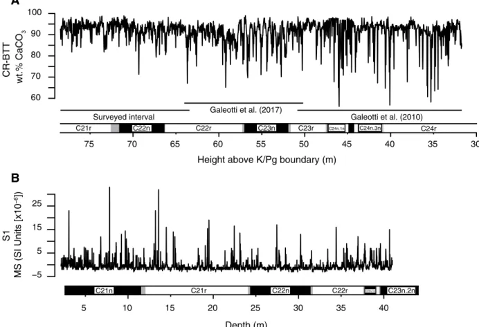
Figure 1.2: Wt.% CaCO3 and δ13C records from the Contessa Road-Bottaccione composite section plotted
against the magnetostratigraphy of both sites. The shaded band represents the marly layer used as a lithostratigraphic marker for the correlation between the two sections.
1.2.2 Magnetostratigraphy
A magnetostratigraphic record of the Contessa Road section up to the lower part of Chron C23n is presented in Galeotti et al. (2010). A highly resolved magnetostratigraphic record was constructed on closely spaced (~25 cm on average) samples taken at Bottaccione in an interval spanning 1.5 m below the marly marker bed to 12.4 m above it, for a total of 61 samples, allowing a precise identification of reversal boundaries with respect to wt.% CaCO3 and stable isotope stratigraphy in the surveyed interval. Measurements
followed standard paleomagnetic procedures, the primary magnetization was isolated from the viscous overprint using principal component analysis after stepwise thermal demagnetization at temperature higher than 350°C. All samples gave a reliable paleomagnetic direction, with antipodal directions that pass a reversal test at the 95% confidence level (Normal Direction: 315.4, 38.7, k = 23.56, N = 29; Reversed
Direction: 142.7, –35.9, k = 23.37, N = 50). The tilt-corrected mean Fisher direction (320, 37, a95 = 3.4) is virtually identical to that reported by Napoleone et al. (1983). Magnetic polarity was interpreted after calculation of the virtual geomagnetic polarity latitude.
Lauretano et al. (2016), to recognise the frequency
modulation of the eccentricity components following
the method described in Laurin et al. (2016).
3. Results
3.1 Magnetostratigraphy
An integrated stratigraphic record of C25n–C23n
in-terval of the Contessa Road record, including bio-
and magnetostratigraphy is discussed in Galeotti et al.
(2000, 2010). Napoleone et al. (1983) published a
bio-and magnetostratigraphic record of the Bottaccione
Eocene. Identification of the original meter marks
used by the latter authors in the field, allows a
straight-forward comparison of our new magnetostratigraphic
record with the available bio- and magnetostratigraphy
(Napoleone et al. 1983). Accordingly, the obtained
paleomagnetic record is very similar to that of Napo
-leone et al. (1983). In particular, we identify two
rever-sals between 51.7–51.8 m and 57.5–57.75 m above
the K/Pg boundary (Fig. 2). The ~ 5.9 m-thick normal
polarity interval delimited by these two reversal
clear-ly corresponds to the C23n magnetochron identified
by Napoleone et al. (1983) between ~ 410–415 m
depth of the original lithostratigraphic log of Arthur
and Fischer (1977), that is ~ 8 m above the lower
boundary of the cherty member of the Scaglia Rossa.
Unfortunately, we were not able to identify the short
reversal separating C23n.1n from C23n.2n. Because
of minor uncertainties in the positioning of the base
of C23n at both sites due to the average sampling
resolution of magnetostratigraphic samples (~ 25 cm),
we use a prominent, 10 cm-thick marly layer in an
otherwise calcareous interval, laying ~ 2 m below the
C23r–C23n magnetochron boundary, whose base is
at 50.25 m above the K/Pg boundary in the Contessa
Road section, as a marker bed to correlate the two
out-crops (Fig. 2). On the other hand, a lithostratigraphic
correlation between the two sites can be easily done
using distinctive marly intervals and other prominent
marly layers that occur in both sections. Comparison
of high-resolution carbon isotope records across the
supposed overlap interval in both sections validates
the litho- and magnetostratigraphic correlations. The
δ
13C record from the two sites shows an optimal match
that allows to confidently obtain a composite section
with a precision in the range of sample resolution
adopted for the geochemistry, i. e. 3 cm (Fig. 2).
The resulting composite section allowed us to
ex-tend the high-resolution record of Galeotti et al. (2010)
to the lower C22r magnetochrons by adding a ~
10m-thick segment sampled at Bottaccione.
Simone Galeotti et al.
234
Fig. 2. Wt.% CaCO
3and δ
13C
records from the Contessa
Road-Bottaccione composite section
plotted against the magnetostrati
-graphy of both sites. The shaded
band represents the marly layer
used as a lithostratigraphic marker
for the correlation between the two
sections.
1.2.3 Geochemistry
Wt.% CaCO3 contents have been measured in a total of 234 samples from the Contessa Road section and
433 samples from the Bottaccione section using a “Dietrich-Frühling” calcimeter with a precision of measurements, based on replicate analyses, within 1%. Sampling resolution was about one sample every 3 cm with a few exceptions across cherty layers where sample resolution was about ~7 cm.
Stable isotope analyses have been carried on bulk samples from the upper part (47.23–54.19 m) of the Contessa Road section encompassing the correlation marl at 50.25 m. Across this interval stable isotope analysis has been conducted on the same sample set used for the analysis of wt.% CaCO3 although with a
resolution of 6 cm for a total of 117 sample. The Bottaccione section was sampled at a resolution of 3 cm for a total of 433 bulk samples. Stable isotope analysis was performed at the IAMC–CNR laboratory (Capo Granitola, Italy) using an automated continuous flow carbonate preparation GasBenchII device and a ThermoElectron Delta Plus V Advantage mass spectrometer on powdered bulk rock samples after heating them at 400°C to remove organic components. Replicate analysis provides a precision within 0.06‰. Carbon isotopes values are calibrated to the Vienna Pee Dee Belemnite standard (VPDB) and converted to conventional delta notation (δ13C).
1.2.4 Spectral analysis
Wavelet analysis of the wt.% CaCO3 record was used to compute the evolutionary spectrum in the depth
domain using the Wavelet Script of Torrence and Compo (1998) and Morlet mother wavelet with an order of 6.
Further, a power spectrum analysis of the CaCO3 was conducted using a 2π-Multi Taper Method
(MTM) with 3 tapers following the method of Ghil et al. (2002). Confidence levels are based on a robust red noise estimation (Mann and Lees, 1996). Moreover, Evolutive Harmonic Analysis (EHA) has been performed on the Contessa Road-Bottaccione (CR-BTT) composite section across the interval that corresponds to the problematic interval defined by Lauretano et al. (2016), to recognise the frequency modulation of the eccentricity components following the method described in Laurin et al. (2016).
1.3 RESULTS
1.3.1 Magnetostratigraphy
An integrated stratigraphic record of C25n–C23n interval of the Contessa Road record, including bio- and magnetostratigraphy is discussed in Galeotti et al. (2000, 2010). Napoleone et al. (1983) published a bio- and magnetostratigraphic record of the Bottaccione Eocene. Identification of the original meter marks used
by the latter authors in the field, allows a straightforward comparison of our new magnetostratigraphic record with the available bio- and magnetostratigraphy (Napoleone et al., 1983). Accordingly, the obtained paleomagnetic record is very similar to that of Napoleone et al. (1983). In particular, we identify two reversals between 51.7–51.8m and 57.5–57.75m above the K/Pg boundary (Fig. 1.2). The ~5.9 m-thick normal polarity interval delimited by these two reversal clearly corresponds to the C23n magnetochron identified by Napoleone et al. (1983) between ~410-415 m depth of the original lithostratigraphic log of Arthur and Fischer (1977), that is ~8 m above the lower boundary of the cherty member of the Scaglia Rossa. Unfortunately, we were not able to identify the short reversal separating C23n.1n from C23n.2n. Because of minor uncertainties in the positioning of the base of C23n at both sites due to the average sampling resolution of magnetostratigraphic samples (~25 cm), we use a prominent, 10 cm-thick marly layer in an otherwise calcareous interval, laying ~2 m below the C23r–C23n magnetochron boundary, whose base is at 50.25 m above the K/Pg boundary in the Contessa Road section, as a marker bed to correlate the two outcrops (Fig. 1.2).
On the other hand, a lithostratigraphic correlation between the two sites can be easily done using distinctive marly intervals and other prominent marly layers that occur in both sections. Comparison of high-resolution carbon isotope records across the supposed overlap interval in both sections validates the litho- and magnetostratigraphic correlations. The δ13C record from the two sites shows an optimal match
that allows to confidently obtain a composite section with a precision in the range of sample resolution adopted for the geochemistry, i.e. 3 cm (Fig. 1.2).
The resulting composite section allowed us to extend the high-resolution record of Galeotti et al. (2010) to the lower C22r magnetochrons by adding a ~10 m-thick segment sampled at Bottaccione.
1.3.2 Geochemical records
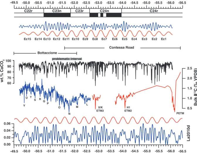
The lower Eocene of the Contessa Road section is characterized by a series of CIEs and concomitant dissolution levels corresponding to the well know succession of early Eocene hyperthermal events, including the Eocene Thermal Maximum 1 (ETM1 or PETM), ETM2 and ETM3 (Galeotti et al., 2000, 2010; Coccioni et al., 2012). In this paper we extend the record of Galeotti et al. (2010) to the lower part of magnetochron C22r, across the stratigraphic segment spanning ~47– 63 m above the K/Pg boundary from the Bottaccione section (Fig. 1.2).
Similar to what is observed across the C24r-C23r interval from the Contessa section (Galeotti et al., 2010), the wt.% CaCO3 record shows a large variability ranging from ~70% to ~98% (Fig. 1.2).
Lowest carbon isotope values are observed at the C23r/C23n boundary where the well-known gradual decline of carbon isotope values, characterising the Early Eocene (Zachos et al., 2008), ends. In this interval the δ13C values range from ~0.3‰ to ~2.0‰, with a rapid rise observed in the middle part of Chron C23n.
increase in the corresponding stratigraphic interval has also been reported by Hilting et al. (2008) based on the analysis of a global stack of benthic data from oceanic records. Moreover, the C23n magnetochron interval is characterized by a series of CIEs (up to 0.6 ‰) similar to those reported for the same age interval at ODP Site 1258 (Demerara Rise) (Kirtland Turner et al., 2014) and ODP Site 1263 (Walvis Ridge - Lauretano et al., 2016).
Notably, as seen in the wt.% CaCO3 record, an interval of increased variance is observed in the δ13C
record across the C23n magnetochron interval. In particular, the δ13C time series shows a variance of
~0.09‰ across the C23n interval, which is 5 times larger than observed in C23r. Comparison between carbon isotope and wt.% CaCO3 records clearly shows that CIEs correspond to carbonate depleted intervals
(Fig. 1.2), suggesting dissolution or dilution across CIEs similar to what observed across hyperthermal events in deeper or marginal settings, respectively.
1.3.3 Spectral analysis
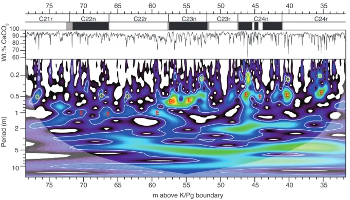
Wavelet analysis of the wt.% CaCO3 record from the CR-BTT composite section reveals that spectral power
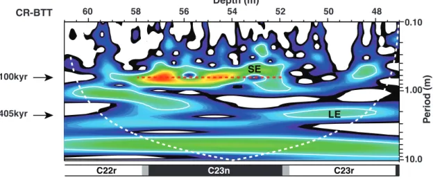
greater than the 95% confidence limit is confined to distinct frequency intervals with periods of ~23 cm, ~50–60 cm and ~200 cm (Fig. 1.3). A decrease in the frequency of the periodic components - centred at about 55 cm - is evident in the wavelet spectrum at ~55 m above the K/Pg boundary, suggesting a corresponding increase in sedimentation rate of the Scaglia limestones. As already evidenced by Galeotti et al. (2010), much power is confined to a frequency interval corresponding to a period of ~5 m in the lower Eocene Contessa Road record, increasing to ~6 m in the surveyed interval.
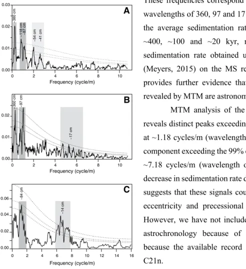
The MTM analysis confirms the results obtained with the wavelet method, providing evidence for distinct spectral peaks above the 95% confidence limit at frequency bands centered at ~1.8, ~4.5 and between ~7–11 cycle/m, which correspond to a period of ~0.55 m, ~0.22 m and ~9–14 cm, respectively. Distinct peaks are also observed at frequencies 0.5 cycle/m and 0.18 cycles/m, thus corresponding to the components with a period of ~ 2 m and 5–6 m, respectively, in the wavelet spectrum (Fig.1.4).
Figure 1.3: Evolutionary wavelet analysis for wt.% CaCO3 values from the CR-BTT composite section for
the interval spanning from 47 to 61 m above the K/Pg boundary and magnetostratigraphy (upper panel). White contours indicate the 99% significance level. Lower panel: wavelet spectrum based on the Fe record from ODP Site 1258 (Westerhold and Röhl, 2009). White contours indicate the 95% significance level. Note the transition to a short eccentricity dominated interval in correspondence to C23n, marked by a red dashed line in both spectra. Notice the transition from a long eccentricity (LE) dominated interval to a short eccentricity (SE) dominated interval at the transition between magnetochrons C23r–C23n at both sites.
Figure 1.4: MTM spectrum of the wt.% CaCO3 record from the CR-BTT composite section. Gray lines
indicate 90%, 95% and 99% confidence levels.
P e riod (m) 0.10 1.00 10.0 C23r C22r 48 50 52 54 58 56 60 Depth (m) C23n LE SE 100kyr 405kyr 100 90 80 70 60 50 P e riod (m) Depth (rmcd) 0.10 1.00 10.0 C23r C 2 2 r C 2 3 n C 2 2 n C 2 4 n 100kyr 405kyr LE SE ODP Site 1258 CR-BTT
Simone Galeotti et al. 236
Fig. 3. Evolutionary wavelet analysis for wt.% CaCO3values from the CR-BTT composite section for the interval spanning from 47 to 61 m above the K/Pg boundary and magnetostratigraphy (upper panel). White contours indicate the 99% signif-icance level. Lower panel: wavelet spectrum based on the Fe record from ODP Site 1258 (Westerhold and Röhl 2009). White contours indicate the 95% significance level. Note the transition to a short eccentricity dominated interval in correspondence to C23n, marked by a red dashed line in both spectra. Notice the transition from a long eccentricity (LE) dominated interval to a short eccentricity (SE) dominated interval at the transition between magnetochrons C23r–C23n at both sites.
Fig. 4. MTM spectrum of the wt.% CaCO3record from the CR-BTT composite section. Gray lines indicate 90%, 95% and 99% confidence levels.
1.4 DISCUSSION
1.4.1 Cyclochronology of the CR-BTT composite section
Both MTM and wavelet analyses provide evidence for the occurrence of periodic components in the wt.% CaCO3 record of the surveyed interval similar to the interval spanning the PETM to the lower part of C23r,
which was deposited at a sedimentation rate of ~0.5 cm/kyr based on the cyclochronology (Galeotti et al., 2010). A similar sedimentation rate value is obtained for the 10 m-thick C23 magnetochron (Fig. 1.2), which according to Vandenberghe et al. (2012) spans ~2 Myr. On this basis, the periodic component recognised through wavelet and MTM spectral analysis can be ascribed to orbital forcing. In particular, the peak with a period centred at ~55cm corresponds to the 100 kyr eccentricity; the peak centred at 22 cm corresponds to obliquity. Moreover, the peaks spread over a frequency range spanning ~7–11 cycle/m are in the precession band.
On the same basis, the large spectral density peaks with periods of ~2m and ~6m correspond to ~400kyr and 1.2Myr. The latter term has already been evidence in the lower Eocene Scaglia Rossa at Gubbio and attributed to a long-term beat of obliquity (Galeotti et al., 2010; DeConto et al., 2012).
The power of these two peaks remains below the 90% confidence limit in the MTM spectrum possibly due to the fact that much power is confined to the short eccentricity component, particularly across C23n, as revealed by the wavelet evolutionary spectrum. However, both peaks are above the 95% confidence limit in the wavelet spectrum. Filtering of the long eccentricity components, hence, can be used to astronomically tune the CR-BTT composite record.
1.4.2 Correlation with ODP Site 1258 and ODP Site 1263
The bulk carbon isotope record from the CR-BTT composite section can be compared to the bulk δ13C
record from ODP Site 1258, Demerara Rise (Kirtland Turner et al., 2014) and the benthic δ13C record from
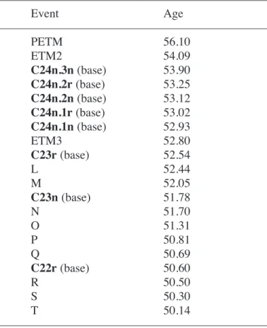
ODP Site 1263, Walvis Ridge (Lauretano et al., 2016). Minor differences in the positioning of individual CIEs with respect to magnetostratigraphy are observed between our record and ODP Site 1258. In particular, C23rH3, or N of Lauretano et al. (2016), which can be easily identified as it occurs at the end of a longer-term decreasing trend in carbon isotope values, falls at the top of C23r at Site 1258 (Kirtland Turner et al., 2014), whereas it is positioned within the lower C23n at Gubbio (Fig. 1.5).
Moreover, the C22rH1 event, or Q according to Lauretano et al. (2016), which occurs at the base of C22r at Site 1258 (Kirtland Turner et al., 2014), falls at the top of C23n at Gubbio (Fig. 1.5).
Unfortunately, no magnetostratigraphy is available from Site 1263 to unravel these minor discrepancies. However, the alignment of the three records is relatively straightforward, which provides a solid basis for chemostratigraphic correlation of the three sites, hence for testing the cyclochronological interpretations