Essays on empirical cultural economics

(1)

Università degli Studi di Sassari

Essays on Empirical Cultural Economics

Direttore della scuola di Dottorato: Prof. Michele M. Comenale Pinto

Tutor:

Prof. Gerardo Marletto

Tesi di Dottorato di Ricerca di: Gianpiero Meloni

La presente tesi è stata prodotta durante la frequenza del corso di dottorato in Diritto ed Economia dei sistemi produttivi dell’Università degli Studi di Sassari, a.a. 2011/2012 - XXVII ciclo, con il supporto di una borsa di studio finanziata con le risorse del P.O.R. SARDEGNA F.S.E. 2007-2013 - Obiettivo competitività regionale e occupazione, Asse IV Capitale umano, Linea di Attività I.3.1.

(2)

(3)

1 Introduction 7 2 American Beauty 12 2.1 Introduction . . . 13 2.2 Data . . . 17 2.3 Methodology . . . 25 2.3.1 Truncation . . . 25 2.3.2 Censored data . . . 27

2.3.3 Sample selection (incidental truncation) . . . 28

2.4 Estimation Results . . . 32

3 La Grande Bellezza 40 3.1 Introduction . . . 41

3.2 Data . . . 42

3.3 Methodology . . . 47

3.3.1 The Poisson regression model . . . 47

3.4 Estimation Results . . . 49

4 Final Remarks 56 5 Appendix I: Data Description 59 5.1 Data description . . . 60

5.1.1 dataset I: American Beauty . . . 60

(4)

6 Appendix II: Script codes 68

6.1 Script I: American Beauty . . . 69

6.1.1 Commented code . . . 69

6.1.2 Naked code . . . 78

6.2 Script II: La Grande Bellezza . . . 86

6.2.1 Commented code . . . 86

6.2.2 Naked code . . . 88

6.3 Commands references . . . 90

(5)

2.1 Movies Descriptive Statistics . . . 18

2.2 Countries Descriptive Statistics: General . . . 21

2.3 Countries Descriptive Statistics: Boxoffice . . . 23

2.4 Determinants of film revenues . . . 35

2.5 Probit results . . . 36

2.6 movie revenues for di↵erent clusters of countries . . . 39

3.1 Movies Descriptive Statistics . . . 44

3.2 Festivals and Prizes . . . 45

3.3 Festivals and Prizes – subsidized movies . . . 46

3.4 Italian movies revenues - base specification . . . 51

3.5 Italian movies revenues - budget iteration with genres . . . 52

3.6 Poisson model for prizes . . . 54

3.7 Poisson model for prizes with iteration between budget and genres . . . 54

7.1 Chamberlain approach - Determinants of film revenues . . . . 92

7.2 Chamberlain approach - movies revenues — HDI groups . . . 92

7.3 Chamberlain approach - movies revenues — CD groups . . . . 93

7.4 OLS of prizes . . . 94

(6)

7.6 Negative binomial model for prizes with iteration between budget and genres . . . 95

(7)

2.1 Movies exhibited per country . . . 19 2.2 Human Development Index versus Cultural Distance . . . 21

(8)

(9)

Movie manufacturing received a lot of attention from academic research in recent years. The role of the market is prominent in the global media industry and its size is increasing: according to PwC1_{, the worldwide revenue}

will grow from 38 billion U.S. dollars in 2014 to nearly 46 billion in 2018. For a practitioner this industry present di↵erent aspects of great interest: DeVany (2004) found that the relationship between a motion picture’s cost and revenue is wildly unpredictable compared to other investments due to the heterogeneity in movie performance with box-office revenues exhibiting heavy right tails. In the words of the author:

The movie industry is a profoundly uncertain business. The prob-ability distributions of movie box-office revenues and profits are characterized by heavy tails and infinite variance! It is hard to imagine making choices in more difficult circumstances. Past suc-cess does not predict future sucsuc-cess. Forecasts of expected rev-enues are meaningless because the possibilities do not converge on a mean; they diverge over the entire outcome space with an infinite variance. This explains precisely why ”nobody knows anything” in the movie business.

A broader motivation for studying motion pictures is that the vast majority of empirical work on trade is for manufacturing, with relatively little work on services. Exports of services such as motion pictures are distinct from exports of manufactures in that variable production costs (e.g., exhibiting movies to consumers) are incurred in the country of consumption, rather than the country of production, and the physical cost of transporting goods abroad (e.g., shipping master film prints) is close to nil. For motion pictures and other cultural goods, cross-country di↵erences in language, social mores, or religion may be the significant barriers to trade (Rauch and Trindade, 2009)2_.

1_Source:

http://www.pwc.com/gx/en/global-entertainment-media-outlook/segment-insights/filmed-entertainment.jhtml

2_{Excerpt from Hanson and Xiang (2011), ”Trade barriers and trade flows with product}

heterogeneity: An application to US motion picture exports”. Journal of International Economics 83, pag 15.

(10)

Aim of the first part of my dissertation, is to highlight the impact of cul-tural di↵erences among importing countries of American movies and how they influence box-office revenues. Previous literature observed the arrival of movies in a country as given (see Lee, 2009) or focused on the determinants of revenues implementing complex econometric procedures like gravity mod-els (Hanson and Xiang 2011, Marvasti and Canterbery 2005) using cultural di↵erences as explanatory variables.

My contribute to the literature comes from the application of the Heckman’s (1979) two-step methodology to infer the probability of arrival of American movies in foreign countries and then to evaluate the box-office revenues for di↵erent clusters of nations built around Hofstede’s (2001) index of cultural distance from the United States and Human Development data (HDI). To do so, I built a data set of 1341 US movies exhibited in 50 countries over the 2002-2013 period: for each of them I collected information on box-office, production budget and idiosyncratic characteristics like genre, sequel, source, Academy Awards nominations and MPAA rating3_.

To sum up the findings discussed in length in Chapter 2, estimation results suggest di↵erent strategies to sell Hollywood movies around the world. In general, countries with relatively high HDI and that are close to the Amer-ican culture tend to be less a↵ected by measures of quality of a movie and show special preferences for action titles. Although the estimation is subject to an identification problem due to the negative correlation between HDI and cultural di↵erences, it suggests that is mostly cultural distance, and not the Human Development level of a country, that leads the consumption in this group of nations. Further, the estimation indicates that once a movie is introduced in a country with low HDI or high cultural distance they are relatively more faithful to the following sequels of these movies.

While Hollywood is the dominant agent in the worldwide movie industry, other markets have a great importance for their size (like India and China in recent years) or their history. The second part of my thesis is devoted to the

3_{Movie ratings from Motion Picture Association of America provide parents with}

ad-vance information about the content of movies to help them determine what’s appropriate for their children. I use this information as a proxy of the content of a movie in terms of violence, sex etc.

(11)

analysis of the Italian movie production market which is one of the oldest in the industry and renowned worldwide for its quality. Academic research on Italian domestic market is, to my knowledge, limited to the contribute of Bagella and Becchetti (1999). With a descriptive and econometric analysis on box office performances of movies produced in Italy between 1985 and 1996, they focused on the relationship between popularity of human inputs and the relative impact of state subsidization on box-office revenues.

Using a GMM-HAC 4 _{approach they find that the ex-ante popularity of}

human inputs (directors and actors) a↵ects in a nonlinear way box-office performance and the interaction between the two factors’ popularity has a positive impact on total admissions. Moreover, authors find that the subsi-dized films do not have a significantly lower performance in the econometric analysis of total admissions and the net e↵ect of subsidies on the mean of the dependent variable is irrelevant.

In chapter 3, La Grande Bellezza, I focus on the impact of state subsidization and try to confirm the results from Bagella and Becchetti looking not only at box-office performances of subsidized movies, but also on their quality. In particular, I collected data for 754 Italian movies exhibited during the 2002-2011 period gathering information on amount of subsidization, genres and festivals presence and related awards granted. Results of box-office rev-enues estimation using subsidization as a single variable are coherent with the findings of Bagella and Becchetti, showing an overall slightly negative im-pact and its net e↵ect is negligible. However, when introducing interaction between subsidies and genres the sign of coefficients turn to be positive and suggest that, while weak, the net impact on public financing on the Italian movie industry is a↵ecting positively box-office revenues.

I find these results to be consistent with the econometric analysis of awards won at festivals where, using a standard Poisson model, iteration variables between genres and subsidies have a slightly positive incidence on the ratio of awards granted. Overall, could be said that public financing is, at least, not hurting the sector and as a policy indication my argue to a better perfor-mance of public expenditure is to shift subsidization on dramas and thrillers

(12)

movies leaving comedies outside of intervention5_.

5_{As shown in Bagella and Becchetti (1999), Italian moviegoers have a strong preference}

(13)

(14)

2.1 Introduction

The field of motion picture industry has received great attention by academic research in the recent period (see McKenzie (2012) for a detailed review); in particular, big focus is given to the transnational flow of motion pictures and the changes in the worldwide supply of movies. In 2007, the New York Times noted that ’American movies (and music) have done very well in some countries like Sweden and less in others like India’. Today, economic growth is booming in countries where American popular culture does not dominate, namely India, China and Russia. Moreover, population growth is strong in many Islamic countries, which typically prefer local culture. Nevertheless, some countries that seem little permeable to foreign cultures, are now ex-periencing an aperture to international movies. After less than three years, The Wall Street Journal (2010) puts in evidence the significant rise of the international box-office and find that this turnabout depends on the fact that ’one of most American of products is now being retooled to suit foreign tastes’. For The Economist (2011) this growth is partially a result of the dollar’s weakness, but it also depends from three crucial aspects: a boom in the demand of movies in the emerging world, a concerted e↵ort by the major studios to produce movies that might play well abroad and a global marketing push to ensure this goal.

One of the first economics studies in the field comes from Prag and Casa-vant (1994) that present an empirical study of the determinants of a motion pictures financial success using a dataset of 652 over a large time period, where a subset of these (195 movies) also have data on advertising expen-ditures. Among the many factors which are included in this study, results that quality and marketing expenditures are important determinants. Film ratings, production cost, and the presence of star performers are only impor-tant determinants when marketing is not included. Marketing expenditures are positively related to production costs, winning Academy awards and the presence of major stars. Looking for simple correlations, the paper states that there is no evidence of a positive relationship between cost of produc-tion and film quality. Also, the only genre dummy which is significant is

(15)

that for dramas and indicates that being a drama is a negative factor for film revenues. Contrary to popular wisdom, PG13 and R rated films do not perform better at the box office.

De Vany and Walls (1999) tried to consider the mathematical properties of box office revenue and estimate profit data of 2.015 movies released between 1985 and 1996 for the United States and Canada and found that is impos-sible to attribute the success of a movie to individual casual factors. They evaluate the impact of budget, actors and director power, sequels, genre, rat-ing and release year on ”hit” probability, where a hit is defined as a movie grossing over US dollars 50 million. They show that the audience reception (captured by a dummy variable for films lasting more than ten weeks) is the most important variable in determining box office revenues. Consequently, they reject forecasting models of box-office revenues.

Marvasti and Canterbery (2005) observe that the American industry motiva-tion for seeking foreign markets is found in his domestic box-office, average costs and industry structure: with remarkably rapid production costs in-crease, di↵erentiation trough export can ensure economies of scale. This can be explained with the fact that most of the marketing costs are incurred for exports that potentially add much more to revenues than to costs. The au-thors state that because of the apparent dependency of domestic box office on a high level of circulating capital is easy to understand the predomi-nance of United States in the movie industry given the di↵erence in gross GDP compared to competitors. This predominance is narrowing due to the changes in GDP observed in countries like China and India. Using an an-nual pooled cross-section dataset of 33 countries over the period 1991-1995 and developing a complex iceberg-gravity model, the authors study the im-pact of cultural and trade barriers to US movies export. They find that despite substantial barriers to film imports, including the low percentual of English-speaking population in the sampled countries, other large economies apparently have been unable to internationally extend their domestic mar-kets. However, data from more recent years, show that this equilibrium is changing and new movie industries are emerging (like China and India). Actually the greatest US barrier to foreign competition appears to be the

(16)

gi-gantic production and marketing costs required to produce the kind of films now demanded around the world.

This chapter aims to study the production function of American movies that sell in foreign markets focusing on the cultural di↵erences among importing countries and the United States. Trade patterns between two countries are usually justified by aspects like national income, which has a positive im-pact, and distance between the two, which impacts negatively1_{. However,}

in recent years, also cultural proximity has been considered like a potential key on international flow between countries. The literature has used di↵er-ent variables to proxy cultural ties, such as common language (Melitz, 2008) or religion (Frankel, 1997). Guiso, Sapienza and Zingales (2009) suggest that ’perceptions rooted in culture are important (and generally omitted) determinants of economic exchange’. In their paper, they show that cultural biases a↵ect economic exchange between countries. This trust is a↵ected not only by the characteristics of the country being trusted, but also by cultural aspects of the match between trusting country and trusted country. The au-thors highlight the e↵ect of trust on bilateral trade in goods, financial assets, and direct foreign investment. Felbermayr and Toubal (2010), similarly, find that cultural proximity is an important determinant of bilateral trade vol-umes of European countries, where cultural distance is measured by bilateral score data from Eurovision Song Contest. Grinblatt and Keloharju (2001) documents that investors are more likely to hold, buy, and sell the stocks of (Finnish) firms that are located close to the investor, that communicate in the investor’s native tongue, and that have chief executives of the same cultural background. As stated by McKenzie and Walls (2012):

A substantial body of work that tests the cultural discount hy-pothesis in the context of the motion-picture industry has evolved over the past decade. Many studies, rely on aggregate or macro-level data to test the cultural discount model. For example, Fu and Sim (2010) and Oh (2001) examined international trade in films and find support for the cultural discount hypothesis.

(17)

Jayakar and Waterman (2000) examined U.S. film exports, and S. W. Lee (2002) examined competitive balance of film trade be-tween the United States and Japan, both studies finding support for the cultural discount hypothesis of media market dominance. Most of the recent studies leverage highly disaggregated film-level data through the application of modern econometric analysis. Fu and Lee (2008) examined the market for films in Singapore, F. L. F. Lee (2006) examined the market for films in Hong Kong, and F. L. F. Lee (2008, 2009) examined the cultural discount hypothesis in a number of East Asian countries. The film-level research uni-formly finds evidence of cultural discount in the particular East Asian motion-picture markets under study.

For the purpose of my analysis, the paper from Lee (2009) is particularly relevant as reported in McKenzie (2012): ”the author takes an interna-tional/cultural perspective on the role of Academy Awards on motion picture demand. Using nominations and awards as indicators of cinematic achieve-ment he investigates the relationship between such achieveachieve-ment and a sample of US films’ box office revenues in nine East Asian countries. In the analy-sis he makes a distinction between ‘drama’ awards (e.g. best director, best leading and supporting actor/actress, best screenplay and best film editing) and ‘non-drama’ awards (all other awards) to investigate how films defined in these respects may have cross-cultural appeal. Using data on the top 100 US movies from 2002 to 2007, the results show that non-drama awards relate positively to box office revenues, but drama awards show negative correla-tions. The interpretation of such results is that films with culturally specific (American) storylines do not translate for East Asian audiences as well as films which, for example, might contain relatively more special e↵ects. Fur-ther, he finds that the negative relationship of drama awards and East Asian box office appears more pronounced in countries less culturally similar to the USA in terms of a culture similarity index.” In his analysis, Lee implemented an approach coming from international management and international trade literature, the Hofstede’s (1980, 2001) cultural dimensions theory, which is a framework for cross-cultural communication that describes the e↵ects of a

(18)

society’s culture on the values of its members, and how these values relate to behavior. As we will see later, I’ll use this framework to group countries in two clusters based on the cultural distance from the United States

2.2 Data

I collected information about di↵erent features including production budget (adjusted for inflation) of 1431 American movies over the period 2002-2013 as well as information on box-office performance for each of them in 50 coun-tries. I focused on this time span, due mainly to the precision of data on foreign markets revenues available on boxofficemojo.com. To measure perfor-mance at box-office for each movie I look at its features splitting in two type of variables: quality variables like budget and Academy Awards nominations in one or more of the main categories2 _{and variables of the idiosyncratic}

features of each title, in particular genres, MPAA ratings3 _{, sequels and}

sources. I gathered these data from opusdata.com and imdb.com, while data for the production budget comes from thenumbers.com4_{.Table 1 shows the}

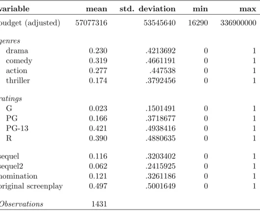
descriptive statistics for the variables under analysis. Note that excluding production budget, all others are dummy variables.

The lowest production budget in the sample belongs to the movie Paranor-mal Activity (16.3 thousands US dollars) which is the most profitable movie ever made in terms of return of investment thanks to a box-office revenue of nearly 200 millions dollars. The biggest budget, 337 millions dollars, cor-responds to the third installment in the Pirates of the Caribbean franchise. Table 1 also shows that the most representative genre is comedy (32% of movies in the sample) which is used as reference category in the estimations.

2_{Best movie, best director, best actor or actress in a leading or supporting role or best}

animation movie.

3_{Movie ratings provide parents with advance information about the content of movies}

to help them determine what’s appropriate for their children and it is used in the sample as a proxy of the content of a movie in terms of violence, sex etc. G stands for Gen-eral Audiences; PG stands for Parental Guidance Suggested; PG-13 stands for Parents Strongly Cautioned; R stands for Restricted, Under 17 requires accompanying parent or adult guardian”

(19)

Table 2.1: Movies Descriptive Statistics

variable mean std. deviation min max budget (adjusted) 57077316 53545640 16290 336900000 genres drama 0.230 .4213692 0 1 comedy 0.319 .4661191 0 1 action 0.277 .447538 0 1 thriller 0.174 .3792456 0 1 ratings G 0.023 .1501491 0 1 PG 0.166 .3718677 0 1 PG-13 0.421 .4938416 0 1 R 0.390 .4880635 0 1 sequel 0.116 .3203402 0 1 sequel2 0.062 .2415925 0 1 nomination 0.121 .3261186 0 1 original screenplay 0.497 .5001649 0 1 Observations 1431

(20)

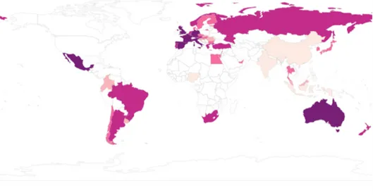
Figure 2.1: Movies exhibited per country

Besides, sequels and franchises account for 18% of the titles in the dataset and an overall 12% received an Academy Awards nomination.

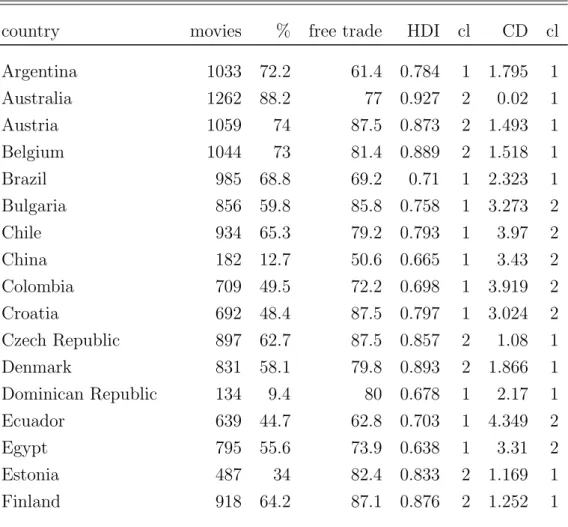
In the second row of Table 2 we can see the number of movies exhibited in each of the 50 countries of our sample, where not surprisingly the nation with more imported film is United Kingdom, followed by Spain, Australia and Germany. The same information is displayed graphically in figure 1. The fourth column shows the mean value over the sample period of the freedom of trade as measured by the Index of Economic Freedom from the Heritage Foundation which constitutes the instrumental variable I use in the probit model to estimate the probability of arrival of a movie i in a country j. In the next section we will see the estimation results for several clusters of countries around two dimensions: Human Development Index (HDI) and cul-tural distance (CD). In particular, for the sake of symmetry the estimation sample is split in two groups depending on the position of each country with respect to the median of the average value of the HDI during the period of analysis and cultural distance, which is fixed through time, which drives to 25 countries for estimation in each of the clusters. The mean values of these

(21)

variables and the relative clusters are shown in columns 5-8 of Table 2. The HDI is an index created by the United Nations and summarizes measure of average achievement in key dimensions of human development: standards of leaving, education and life’s expectation and quality. According to the Human Development Index technical notes in our sample there is one low developed country (Nigeria, < .500), ten medium developed nations (>= .500 and < .700), thirteen high developed (>= .700 and < .800) and twenty-six very highly developed countries (>= .800). To capture information about the cultural distance between U.S.and each of the countries in the dataset, following Lee (2009), I implement a value-based index developed by Hofstede (1980) built around four dimensions: 1) power distance, that expresses the degree to which the less powerful members of a society accept and expect that power is distributed unequally; 2) uncertainty avoidance expresses the degree to which the members of a society feel uncomfortable with uncertainty and ambiguity; 3) individualism versus collectivism and 4) masculinity ver-sus femininity5_{. I gathered data for each country and values from Hofstede}

(2001) and then each country’s cultural distance from the United States is computed using Kogut and Singh’s (1988) formula:

CDj =

X

I=1

(Iij Iiu)2/Vi /4

Where CDj is the cultural distance of country j from the United States, Iij

is the value for country j on the ith cultural dimension (Iiu for the U.S.) and

Vi is the variance of the ith cultural dimension. A simple correlation analysis

shows that there is a positive correlation between HDI and the number of movies exhibited in a country that is also negatively correlated with the cultural distance from US. Besides, there is a negative correlation between HDI and CD, in fact in a regression between these variables, the coefficient associated to cultural distance is 0.02 with a p-value equal to 0.048. Figure 1 shows the values of these two variables for the 50 countries.

5_{See section I of the Appendix for a briefer description of this index and all other}

(22)

Figure 2.2: Human Development Index versus Cultural Distance

Table 2.2: Countries Descriptive Statistics: General

country movies % free trade HDI cl CD cl

Argentina 1033 72.2 61.4 0.784 1 1.795 1 Australia 1262 88.2 77 0.927 2 0.02 1 Austria 1059 74 87.5 0.873 2 1.493 1 Belgium 1044 73 81.4 0.889 2 1.518 1 Brazil 985 68.8 69.2 0.71 1 2.323 1 Bulgaria 856 59.8 85.8 0.758 1 3.273 2 Chile 934 65.3 79.2 0.793 1 3.97 2 China 182 12.7 50.6 0.665 1 3.43 2 Colombia 709 49.5 72.2 0.698 1 3.919 2 Croatia 692 48.4 87.5 0.797 1 3.024 2 Czech Republic 897 62.7 87.5 0.857 2 1.08 1 Denmark 831 58.1 79.8 0.893 2 1.866 1 Dominican Republic 134 9.4 80 0.678 1 2.17 1 Ecuador 639 44.7 62.8 0.703 1 4.349 2 Egypt 795 55.6 73.9 0.638 1 3.31 2 Estonia 487 34 82.4 0.833 2 1.169 1 Finland 918 64.2 87.1 0.876 2 1.252 1

(23)

France 1214 84.8 81 0.877 2 1.524 1 Germany 1236 86.4 86 0.899 2 0.472 1 Greece 956 66.8 80.2 0.85 2 3.749 2 Hungary 853 59.6 87.1 0.815 2 1.062 1 India 374 26.1 24.2 0.526 1 1.637 1 Indonesia 404 28.2 74.6 0.598 1 3.822 2 Israel 543 37.9 77.1 0.887 2 1.73 1 Italy 1215 84.9 86.8 0.865 2 0.58 1 Jamaica 151 10.6 70.4 0.705 1 1.874 1 Japan 761 53.2 80.6 0.895 2 2.704 2 Kuwait 151 10.6 77.8 0.786 1 4.217 2 Lebanon 877 61.3 80.5 0.738 1 1.916 1 Malaysia 661 46.2 73.4 0.754 1 4.264 2 Mexico 1230 86 57.6 0.749 1 3.303 2 Netherlands 1085 75.8 87.5 0.907 2 1.437 1 New Zealand 1127 78.8 84.6 0.905 2 0.246 1 Nigeria 411 28.7 61.6 0.465 1 2.686 2 Norway 965 67.4 89.2 0.943 2 2 1 Portugal 1006 70.3 79.8 0.806 1 4.391 2 Romania 617 43.1 86 0.767 1 4.204 2 Russia 1049 73.3 62.6 0.76 1 4.223 2 Singapore 875 61.1 85 0.876 2 3.854 2 Slovakia 635 44.4 87.1 0.825 2 4.151 2 Slovenia 654 45.7 86.5 0.88 2 4.402 2 South Africa 1095 76.5 76.3 0.622 1 0.382 1 South Korea 825 57.7 73.6 0.882 2 3.854 2 Spain 1302 91 79.8 0.867 2 1.9 1 Sweden 883 61.7 87.1 0.906 2 2.278 1 Thailand 792 55.3 75.9 0.676 1 3.405 2

(24)

Turkey 965 67.4 73.7 0.697 1 2.647 2

United Arab Emirates 915 63.9 75 0.824 2 4.017 2

United Kingdom 1316 92 87.6 0.865 2 0.079 1

Uruguay 674 47.1 83 0.776 1 3.385 2

Observations 41274

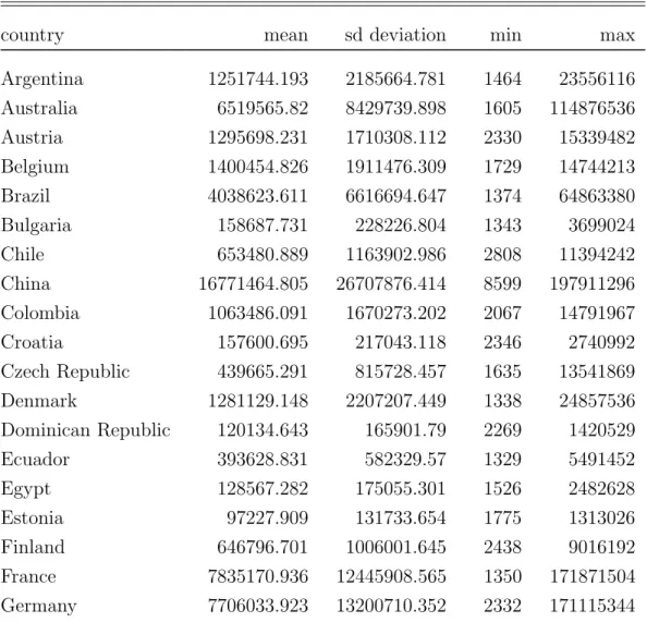
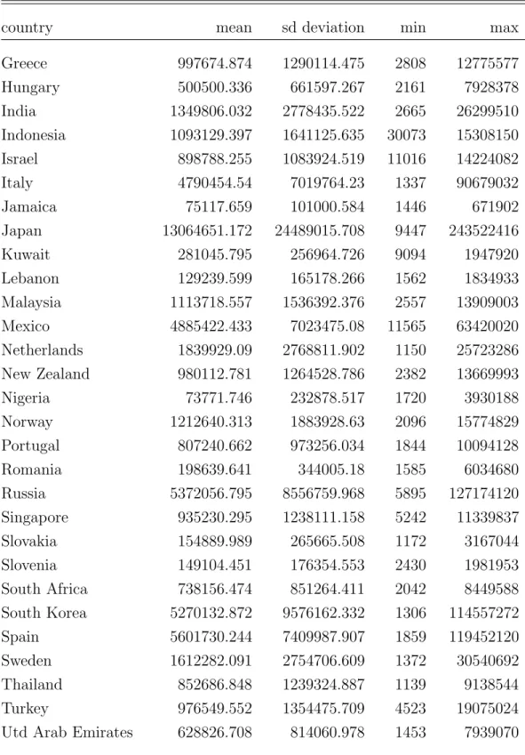
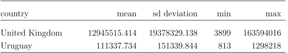
Table 2.3: Countries Descriptive Statistics: Boxoffice

country mean sd deviation min max

Argentina 1251744.193 2185664.781 1464 23556116 Australia 6519565.82 8429739.898 1605 114876536 Austria 1295698.231 1710308.112 2330 15339482 Belgium 1400454.826 1911476.309 1729 14744213 Brazil 4038623.611 6616694.647 1374 64863380 Bulgaria 158687.731 228226.804 1343 3699024 Chile 653480.889 1163902.986 2808 11394242 China 16771464.805 26707876.414 8599 197911296 Colombia 1063486.091 1670273.202 2067 14791967 Croatia 157600.695 217043.118 2346 2740992 Czech Republic 439665.291 815728.457 1635 13541869 Denmark 1281129.148 2207207.449 1338 24857536 Dominican Republic 120134.643 165901.79 2269 1420529 Ecuador 393628.831 582329.57 1329 5491452 Egypt 128567.282 175055.301 1526 2482628 Estonia 97227.909 131733.654 1775 1313026 Finland 646796.701 1006001.645 2438 9016192 France 7835170.936 12445908.565 1350 171871504 Germany 7706033.923 13200710.352 2332 171115344

(25)

Greece 997674.874 1290114.475 2808 12775577 Hungary 500500.336 661597.267 2161 7928378 India 1349806.032 2778435.522 2665 26299510 Indonesia 1093129.397 1641125.635 30073 15308150 Israel 898788.255 1083924.519 11016 14224082 Italy 4790454.54 7019764.23 1337 90679032 Jamaica 75117.659 101000.584 1446 671902 Japan 13064651.172 24489015.708 9447 243522416 Kuwait 281045.795 256964.726 9094 1947920 Lebanon 129239.599 165178.266 1562 1834933 Malaysia 1113718.557 1536392.376 2557 13909003 Mexico 4885422.433 7023475.08 11565 63420020 Netherlands 1839929.09 2768811.902 1150 25723286 New Zealand 980112.781 1264528.786 2382 13669993 Nigeria 73771.746 232878.517 1720 3930188 Norway 1212640.313 1883928.63 2096 15774829 Portugal 807240.662 973256.034 1844 10094128 Romania 198639.641 344005.18 1585 6034680 Russia 5372056.795 8556759.968 5895 127174120 Singapore 935230.295 1238111.158 5242 11339837 Slovakia 154889.989 265665.508 1172 3167044 Slovenia 149104.451 176354.553 2430 1981953 South Africa 738156.474 851264.411 2042 8449588 South Korea 5270132.872 9576162.332 1306 114557272 Spain 5601730.244 7409987.907 1859 119452120 Sweden 1612282.091 2754706.609 1372 30540692 Thailand 852686.848 1239324.887 1139 9138544 Turkey 976549.552 1354475.709 4523 19075024

(26)

United Kingdom 12945515.414 19378329.138 3899 163594016

Uruguay 111337.734 151339.844 813 1298218

2.3 Methodology

The non-random nature of the sample population put some challenges for the empirical analysis. The principal issue is that not every movie is shown in each country and as a consequence the panel is not balanced. This could lead to endogenous sample selection resulting in inconsistent estimates of the coefficient if, within a model of the revenue performance, the variables that a↵ect the probability of arrival of a movie in a certain country are also highly correlated with the revenue of that movie. The best practice in this kind of scenario is to implement the Heckman’s (1979) two-step estimation procedure. This section provides the theoretical background of the sample selection problem starting from its two principal components, truncated and censored distributions6_.

2.3.1 Truncation

A truncated distribution is the part of an untruncated distribution that is above or below some specified value. For instance, in the sample under anal-ysis, I could subset the population cutting o↵ those movies with a production budget below one million dollars. In order to derive the first and second mo-ments of the truncated distribution we must introduce first the density of a truncated random variable.

Theorem 1 (Density of a Truncated Random Variable). If a continuous random variable x has a probability density function f (x) and a is a constant,

6_{Notation and order of the arguments follow Greene (2003) Econometric Analysis}

(27)

then

f (x_{|x > a) =} f (x) P rob(x > a)

If x has a normal distribution with mean µ and standard deviation , then

P rob(x > a) = 1 ✓

a µ◆

= 1 (↵)

where ↵ = (a µ)/ and (·) is the standard normal cumulative density function. The density of the truncated normal distribution is then

f (x|x > a) = f (x) 1 (↵) = (2⇡ 2₎ 1/2_e (x µ)2_/(2 2₎ 1 (↵) = 1 ✓a µ◆ 1 (↵)

where (·) is the standard normal pdf.

We can now derive the moments of a truncated normal distribution as follows: Theorem 2 (Moments of the Truncated Normal Distribution). If x_{⇠ N[µ,} 2_]

and a is a constant, then

E[x|truncation] = µ + (↵), V ar[x|truncation] = 2_[1 _(↵)],

where ↵ = (a µ)/ , (↵) is the standard normal density and

(↵) =

1 (↵) if truncation is x > a, and

(↵) = (↵)[ (↵) ↵] with 2 (0, 1).

The function (↵) called the inverse Mills Ratio7_{, named after John P.}

Mills, as we can see from the formula is the ratio of the probability density function to the cumulative distribution function of a distribution. Its role is crucial in the following regression analysis to take in account of possible

(28)

selection bias, as proposed by Heckman (1979).

2.3.2 Censored data

Censoring is a condition in which the value of an observation is only partially known. When the dependent variable is censored, values in a certain range are all transformed to a single value. This point will be useful in the next subsection when, modeling the probability of exhibition of a movie in a cer-tain country, we define the selection variable z⇤. Meanwhile, let derive the censored normal distribution as we did for truncation. Define a new random variable y as a transformation of the original one y⇤ _by

y = 0 if y⇤  0 y = y⇤ if y⇤ > 0 The distribution that applies if y⇤ _{⇠ N[µ,} 2_{] is}

P rob(y = 0) = P rob(y⇤ _{ 0) =} ⇣ µ⌘= 1 ⇣µ⌘, and, if y⇤ _{> 0, then y has the density of y}⇤_.

Theorem 3 (Moments of the Censored Normal Variable). If y⇤ _{⇠ N[µ,} 2_]

and y = a if y⇤ _{ a or else y = y}⇤_{, then}

E[y] = a + (1 )(µ + ) V ar[y] = 2(1 )[(1 ) + (↵ )2 ] where [(a µ)] = (↵) = P rob(y⇤  a) = , = (1 ) and = 2 _↵.

(29)

2.3.3 Sample selection (incidental truncation)

Many samples are truncated on the basis of a variable that is correlated with the dependent variable. For example, let assume that the international distribution of a movie is set by the production companies only that choose to export a film in a country if the expected revenue exceeds their reservation revenue and choose to stay out of that country otherwise8_{. If the dependent}

variable (box-office revenues in my sample) is correlated with the di↵erence between reservation and expected revenues, least squares yields inconsistent estimates. In this case, the sample is said to have been selected on the basis of this di↵erence.

Suppose that y and z have a bivariate distribution with correlation ⇢. With respect to the previous example, we are interested in the distribution of y given that z exceeds a particular value. As before, we are interested in the form of the incidentally truncated distribution and the mean and variance of the incidentally truncated random variable.

The truncated joint density of y and z is

f (y, z_{|z > a) =} f (y, z) P rob(z > a)

To obtain the incidentally truncated marginal density for y, we would then integrate z out of this expression. The moments of the incidentally truncated normal distribution are given in the following theorem.

Theorem 4 (Moments of the Incidentally Truncated Bivariate Normal Dis-tribution). If y and z have a bivariate normal distribution with means µy

and µz, standard deviations y and z, and correlation ⇢, then

E[y|z > a] = µy+ ⇢ y (↵z),

V ar[y|z > a] = 2

y[1 ⇢2 (↵z)

8_{Note that this kind of assumption is not realistic as it neglect the importing decision}

(30)

where ↵z = (a µz) z , (↵z) = (↵z) [1 (↵z)] and (↵z) = (↵z)[ (↵z) ↵z]

We are now able to derive a general framework, let z⇤_i = www000i + ui

be the equation that determines the sample selection and y⇤_i = xxx000i + "i

the equation of primary interest. "i and uihave bivariate normal distribution

with zero means and correlation ⇢. The sample rule is that yi is observed

only when z_i⇤ > 0. Applying Theorem 4 we obtain the model E[yi|yi is observed] = E[yi|zi⇤ > 0]

If is omitted the specification error of an omitted variable is committed and the OLS regression produces inconsistent estimations of .

(31)

observe only its sign, but not its magnitude. The absence of information on the scale of z⇤ _{implies that the disturbance variance in the selection equation}

cannot be estimated. Thus, a reformulation of the model is mandatory. Let assume that zi and wwwi are observed for a random sample of observations but

yi is observed only when zi = 1, then selection mechanism becomes:

z⇤ i = www000i + ui with ( zi = 1 if zi⇤ > 0 zi = 0 otherwise P rob(zi = 1|www) = (www000i ) P rob(zi = 0|www) = 1 (www000i )

Then the regression model is y⇤_i = xx_x000

i + "i observed only if z = 1

(ui, zi)⇠ bivariate normal[0, 0, 1, ", ⇢]

with

E[yi|zi, xxxi, wwwi] = xxx000i + ⇢ " (www000i )

The parameters of the sample selection model are usually estimated using Heckman’s (1979) two-step procedure9 _{that works as follows:}

1. Estimate the probit equation by maximum likelihood to obtain esti-mates of . For each observation in the sample compute the inverse Mills ratio ˆi = (www000iˆ)/ (www000iˆ)

2. Estimate and = ⇢ " by least squares regression of y on xxx and ˆ.

The probit model belongs to the family of binary response models that are used when the dependent variable is dichotomic, so that can take only two values and is usually coded as 0 and 1. Typical economic examples are the participation to the labor force, in which an agent chooses between two alternatives or di↵erences in wage related to gender, in which being a female or a male can drive to di↵erent salaries. If we consider the sample of American

(32)

movies under analysis, the dependent variable will take value 1 if a movie is exhibited in a certain country and 0 otherwise. Let Pi be the probability

that yi = 1 conditional on the information set ⌦i, which is characterized

by exogenous variables. The aim is to model the conditional probability and since the values of the dependent variables are 0 and 1, Pi is also the

expectation of yi conditional on ⌦i10

Pi ⌘ (yt= 1 | ⌦i) = E(yt= 1 | ⌦i)

It is important to understand why the implementation of a regression model is note feasible when we face this kind of dependent variable: suppose that Xi ⇢ ⌦i is a row vector of length k in which the first term is a constant.

Then a linear regression model would specify E(yi = 1| ⌦i) as Xi , failing to

impose the condition that 0 E(yi = 1 | ⌦i) 1, which must holds because

E(yi = 1 | ⌦i) is a probability. And since it makes no sense to estimate

negative probabilities or greater than 1, regressing yi on Xi is not a feasible

approach to model the conditional expectation of a binary variable. To ensure that Pi 2 [0, 1], a model must specify that:

Pi ⌘ E(yi = 1| ⌦i) = F (Xi ).

Where Xi is an index function which maps from the vector of explanatory

variables Xi and the vector of parameters to a scalar index, and F (x) is a

transformation function with the following properties:

F ( _{1) = 0, F (1) = 1, f(x) ⌘} dF (x) dx > 0

Which are the properties of the cumulative distribution function of a proba-bility distribution, and ensure that F (Xi )2 [0, 1] while allowing the index

function Xi to take any value on the real line.

10_{Thus a binary response model can also be thought of as modeling the conditional}

(33)

A binary response model is a probit when F (Xi ) = (Xi ) where ⌘ p1 2⇡ Z x 1 exp ✓ 1 2X 2 ◆ dX

and its first derivative is the standard normal density function (x). An attractive feature of the probit model is that it can be derived from a model involving a latent, unobserved, variable z⇤

i.As seen before, let be

z_i⇤ = Xi + ui, ui ⇠ NID(0, 1).

We observe only the sign of z⇤

i, which determines the value of the observed

binary variable yi with the relationship

yi = 1 if z⇤i > 0; yi = 1 if zi⇤  0

The two previous equations define a latent variable model, the intuition is that z⇤

i is an index of the net utility associated with some action; only if its

value is positive then the action is undertaken. Then it is now possible to compute Pi, the probability that yi = 1 as

P (yi = 1) = P (zi⇤ > 0) = P (Xi + ui > 0)

= P (ui  Xi ) = (Xi ).

2.4 Estimation Results

A general approach in economic literature explains film success as a function of production budget, awarded prizes and features of the movie like genre, rating, being a sequel and so on. This approach is particularly useful when it is applied to countries abroad the United States given that, although the di↵erent explanatory variables may fail to be exogenous in the local market as the can be deemed to be a↵ected by the expected revenue, in general they can be considered as exogenous with respect to the revenue in each single country.

(34)

Therefore the baseline specification explains the revenue of a movie i (in logs and adjusted for inflation) in a country j as a function of two main groups of variables: indicators of the quality of the film, budgeti and nominationi

and variables related to the di↵erent features of a movie in order to check how these characteristics have an impact on its box-office performance. The following model is considered:

ln revenueij = 0+ 1ln budgeti+ 2nominationi+ 3sequeli+ 4f ranchisei

+ 5ratingsi+ 6genresi+ 7originali+ yeari+ countryj+ ✏i

where budgeti is the log of the production budget for the ith film expressed

in American dollars and adjusted for inflation; nominationi is a dummy

variable that takes value 1 if the ith movie received an Academy Award Nomination in one or more of the main categories: best movie, best director, best actor or actress in a leading or supporting role or best animation movie; sequeli and f ranchisei denote if the ith is a sequel or a subsequent title

in a serie; ratingsi is a vector of dummy variables that includes Gi, P Gi

and Ri, that according to the MPAA Film Rating System stands for general

audience, parental guidance suggested and parents strongly cautioned respec-tively; genres_i is a vector that includes dramai, actioni, thrilleri; originali

is a factor variable which takes value 1 if the screenplay is an original sub-ject and 0 otherwise; countryj and yeari are included to control for di↵erent

unobserved factors that could explain heterogeneity of movies revenues in di↵erent nations and time periods; the terms r for r = [1, 7] are parameters

of the model and ✏i,j is an error term.11

The sample amounts to 1431 US movies observed in a total of 50 di↵erent countries, where US/Canada is not included12_{, from 2002 and 2013.}

How-ever, the panel is not balanced because not every movie is shown in each of the countries. The possible presence of endogenous sample selection may then result in inconsistent estimates of the coefficients in a model that

ac-11_{Variables P G} ₁₃

i and commedyi are leaved outside age rating and genre groups

respectively to avoid perfect multicollinearity.

12_{MPAA, www.boxeofficemojo.com and other data providers aggregate United States}

(35)

counts for film revenues if the shock that a↵ect the probability that a given film is exhibited in a certain country are highly correlated with the shocks that determines its revenue. Based on this premise I run an estimation pool model for film revenues in all countries employing Heckman’s (1979) two-step methodology. In the first step, I estimate a probit model for the probability that a movie is exhibited in a country; this allows to obtain the Mills ratios needed to correct the OLS estimates of the primary equation in the second stage. In order to identify the model it is necessary to choose at least one instrumental variable to be included only in the probit correlated with the probability of exhibition but uncorrelated with the unobservable error term. A first best solution is to use information about entry barriers for foreign movies in each country: an important advantage of this type of variable is that given it has been defined at national level it is plausible to assume that it is exogenous to the expected revenue of each individual movie. However, note that protection laws in favor of local movie industries could come in a variety of di↵erent forms such as definitions of quotas for foreign movies like in France. Also, some of these laws are quite old (in Italy one should trace back to 1936) and, while are still in place, are not actively applied. Although it is impossible to get enough information about all the possible types of restrictions in the film industry for each country in the sample, this informa-tion can be successfully proxied by the trade of freedom index included in the Economic Freedom report of the Heritage Foundation. Beside this variable I also considered the inclusion of two alternative instruments defined at movie level: 1) opening week revenue in the domestic market13_{; and 2) an indicator}

of whether the nearest neighbor movie released in a particular country two years before.14_{. However, over-identifying tests clearly indicates that these}

are not valid instruments as they are both significant at the conventional levels in the primary equation.

Table 1.4 shows the results of equation (1) for both the Heckman model and a typical OLS estimation of a pool regression for the 50 countries in the sample.

13_{see McKenzie and Walls (2012).}

14_{The definition of this variable is based on the minimization of the canonical distance}

of each film with all other movies exhibited two years earlier using the same variables defined in equation (1) and it was implemented by R package FNN.

(36)

Results from the probit model estimation are reported in table 1.5 and can

Table 2.4: Determinants of film revenues

Heckit model OLS regression budget 0.933(***) (62.67) 0.640(***) (55.58) nomination 0.973(***) (38.62) 0.637(***) (35.52) drama -0.290(***) (-13.17) -0.258(***) (-11.74) action 0.331(***) (17.63) 0.236(***) (13.43) thriller 0.479(***) (20.87) 0.267(***) (14.01) G -0.0886(*) (-2.29) 0.0392 (1.03) PG -0.00379 (-0.21) 0.0460(**) (2.60) R -0.0658(***) (-4.49) -0.0489(***) (-3.31) sequel 0.582(***) (28.01) 0.469(***) (23.80) sequel2 0.530(***) (22.38) 0.427(***) (18.60) Inverse Mills Ratio 1.409(***) (18.53)

N 41274 41274

Adjusted R2 _0.615 _0.610

Omitted: comedy, PG-13; t statistics in parentheses. (*) p < 0.05, (**) p < 0.01, (***) p < 0.001

be seen that the estimated coefficient associated to the instrumental variable trade freedom is positive and significant at the conventional values and the qualitative impact of all other variables is similar to their estimated e↵ect in the revenue equation. I find evidence of endogenous samples selection as the inverse mills ratio is highly significant in the primary equation and has a positive sign which is consistent with the logical argument that films that are expected to have higher revenue in a given country are also more likely to be exhibited there.

However, in spite of these findings, the comparison with the OLS esti-mation indicates that most of the qualitative results are una↵ected by the Heckman correction. To control for potential correlation of the error term in the primary and selection equations I also tested the Mundlak-Chamberlain approach as proposed by Wooldridge (2010), with no qualitative change in

(37)

Table 2.5: Probit results trade freedom 0.015(*) (2.23) budget 0.933(***) (62.67) nomination 0.973(***) (38.62) drama -0.290(***) (-13.17) action 0.331(***) (17.63) thriller 0.479(***) (20.87) G -0.0886(*) (-2.29) PG -0.00379 (-0.21) R -0.0658(***) (-4.49) sequel 0.582(***) (28.01) sequel2 0.530(***) (22.38) original screenplay 0.0462(***) (3.63) N 41274

Omitted: comedy, PG-13; t statistics in parentheses. (*) p < 0.05, (**) p < 0.01, (***) p < 0.001

(38)

the estimated results or in the subsequent ranking of countries presented next.

It can be observed that variables related to the quality of a movie such as budget and nomination have a positive impact both in the revenue and the probability of exhibition. Moreover, mild movies for the general audi-ence are less successful in terms of revenue than stronger movies for which parental guidance is suggested which seems to indicate that, at least outside the domestic market, Hollywood movies are not mainly produced for family consumption as in principle one could suggest. The fact that sequels and subsequent movies in a serie have a positive impact on revenue outlines that it is profitable in many circumstances to take advantage of an existing prod-uct instead of introducing a completely new movie in the market (and with that new characters and plots). Should be noted that drama movies are less profitable than other genres such as thriller and action movies.

Although I control for country individual e↵ects in the above estimation, there is a risk of aggregation bias given that the model imposes that ex-planatory variables have the same impact on revenues regardless the type of country under analysis. In a first approximation to circumvent this problem I estimate equation (1) for two groups of countries depending on their human development level and cultural distance to the United States. In particular, for the sake of symmetry the estimation sample is split in two groups depend-ing on the position of each country with respect to the median of the average value of the HDI during the period of analysis and cultural distance, which is fixed through time, which drives to 25 countries for estimation in each of the clusters. The estimation output is shown in Table 1.6. Note that estimated parameters for countries with high HDI are very similar to countries that are close to the American culture. In fact, there is a high correlation between these two groups of countries that can be observed in the fact that for the 25 countries with HDI over the median, 18 have a CD below the median. In general, countries with high HDI (or with low CD) see to be less a↵ected by nomination and budget that which points to the fact they are more prone to consume all type of American movies instead of only high quality ones. Another potential explanation for this result is that more developed

(39)

coun-tries could be interested in less commercial movies. Besides, high HDI and low CD countries dislike relatively more mild films that are authorized for all the public which is probably an indication that society is less restrictive in these countries; surprisingly they are less faithful to sequels, suggesting that they have more alternative leisure options to previous successful movies. Regarding their taste about genres, countries in the high HDI and low CD cluster show relatively more preferences for action films and less preferences for drama (with respect to comedies).

One possible way to circumvent the identification problem about the role played by HDI and CD to explain tastes for US movies is to estimate the previous equation only for countries with HDI above the median but that are not close to the American culture (Greece, Japan, Singapore, Slovakia, Slovenia, South Korea and United Arab Emirates) and for countries with HDI below the median and low CD (Argentina, Brazil, Dominican Republic, India, Jamaica, Lebanon and South Africa). Results of this estimation are shown in Table 1.6. Note that estimation results for countries with a cultural proximity to the United States but with low HDI are more similar to the av-erage estimation for high and low CD shown in columns 1 and 4 of table 1.6. On the contrary, nations with high HDI and high CD show higher preference for budget and nomination as they are relatively more attracted by only high quality movies, less preference for mild films and more preference for drama, action and thriller movies with respect to the reference genre, comedy. In fact, comedies have typically very idiosyncratic values that makes them dif-ficult to export to countries with di↵erent cultural values.

(40)

Ta b le 2. 6: m ov ie re ve n u es fo r d i↵ er en t cl u st er s of co u n tr ie s lo w H DI high H DI high CD lo w CD high H DI /CD lo w H DI /C D budget 0.896*** (39.71) 0.973*** (49.81) 0.954*** (46.77) 0.972*** (41.78) 1.095*** (19.83) 0.802*** (16.33) nomination 0.689*** (19.85) 1.220*** (33.37) 1.228*** (33.86) 0.742*** (19.94) 0.946*** (10.33) 0.729*** (10.44) drama -0.372** * (-12 .1 6) -0.239*** (-7.88) -0.264*** (-8.61) -0.345*** (-11.32) -0.192*** (-3.33) -0.307*** (-5.33) action 0.356*** (12.88) 0.301*** (11.91) 0.230*** (9.33) 0 .4 46*** (15.25) 0.534* ** (8.08 ) 0.190*** (3.55) thriller 0.525*** (14.99) 0.437*** (14.44) 0.345*** (11.59) 0.669*** (18.09) 0.78 5*** (9.13) 0.236*** (3.37) G-0 .3 1 4 * * * (-5 .6 0 ) 0 .0 7 9 1 (1 .5 3 ) 0 .0 8 6 3 (1 .6 7 ) -0 .3 3 1 * * * (-5 .8 8 ) -0 .4 0 6 * * * (-3 .5 4 ) -0 .2 9 6 * (-2 .4 7 ) PG 0. 0269 (1. 17) -0 .0 393 (-1 .5 3) -0. 0300 (-1. 15) 0. 00960 (0. 42) -0. 0902 (-1. 94) -0. 0129 (-0. 28) R-0 .1 8 5 * * * (-8 .6 5 ) 0 .0 2 9 8 (1 .4 7 ) 0 .0 0 9 4 5 (0 .4 6 ) -0 .1 6 0 * * * (-7 .6 7 ) -0 .1 3 2 * * * (-3 .3 3 ) -0 .1 9 7 * * * (-4 .1 5 ) seq uel 0.522*** (18.33) 0.638* ** (21 .8 5) 0.666*** (22.34) 0.511*** (17.79) 0.528*** (8.97) 0.541*** (8.91) seq uel2 0.444*** (12.97) 0.603*** (18.60) 0.596*** (18.05) 0.468 *** (1 3.78) 0.516*** (7.86) 0.439*** (6.26) original screenpla y 0.0903*** (5.19) 0.0084 8 (0.47) 0.0139 (0.76) 0.0831*** (4.79) 0.05 59 (1.65 ) 0.0790* (2.28) Inverse Mil ls R atio 1.233*** (10.84) 1.609*** (15.40) 1.631*** (13.95) 1.427*** (12.82) 1.741*** (6.46) 0.836** (2.71) cons -4.272*** (-8.64) -3.469*** (-8.70) -5.313 *** (-12.29) -8.026*** (-15.08) -8.284*** (-6.55) -2.101 (-1.95) Observ ations 1741 6 23858 22886 18388 56 21 4649 Ad ju st ed R 2 0.658 0.559 0.562 0.659 0.625 0.619 O mi tt e d : c o me d y , P G -1 3 ; t st a tist ic s in pa re n the se s. (*) p< 0 .05, (**) p< 0 .01, (***) p< 0 .001

(41)

(42)

3.1 Introduction

The Italian film industry is pretty active in terms of movies produced per year. The Anica report for 20111 _{shows that domestic theaters exhibited}

241 titles entirely produced in Italy plus 55 co-produced with other countries over a total of 901 exhibited movies2_{. However, to my knowledge, academic}

research on the field didn’t pay much attention to this market.

The only notable exception comes from Bagella and Becchetti’s (1999) paper that studies some of the critical issues in the Italian movies market with a descriptive and econometric analysis on box office performances of movies produced in Italy between 1985 and 1996. In particular they focused on the relationship between popularity of human inputs (director and cast of actors) and box office revenues and the specialization in comedy production.

They use a database which gathers information on all movies produced in Italy from 1985 to 1996 with a sample of 977 films. For each movie they con-sider producing or co-producing companies, total admissions, distribution companies, box office revenues and programming days, ex ante popularity of actors and directors and availability of state subsidies. The total number of admissions is used as a dependent variable to measure box office performance. The descriptive analysis presented documents a reduction in the number of movies financed in the relevant sample period, and a sharp reduction in per screen daily admissions and revenues, paralleled by a positive trend in ab-solute admissions. In the econometric analysis the focus is on three crucial issues: the first is relative to how popularity of human inputs a↵ects motion picture performance. The second is on the relative impact of state subsidiza-tion, while the third regards the relative impact of additional factors such as organizational and marketing capacity of production houses and the Italian viewers taste specificity a↵ecting the relate success of specialization genres. Using a GMM-HAC (Generalized Method of Moments Heteroskedasticity and Autocorrelation Consistent) approach they find that the ex-ante popu-larity of human inputs a↵ects in a nonlinear way box-office performance and

1_{www.anica.it/online/allegati/dati/19042012 DATI2011.pdf}

2_{313 movies came from United States, 226 from other European countries and 66 from}

(43)

the interaction between the two factors’ popularity has a positive impact on total admissions. With regard to the second question, a quite surprising result shows that the subsidized films do not have a significantly lower per-formance in the econometric analysis of total admissions, daily revenues and per screen daily admissions despite the far lower ex ante popularity of cast and directors of subsidized films as compared to non subsidized films. As for the third question, when looking at the results on net impact of di↵erent Italian production houses on the dependent variable, they find that only one (Filmauro) has a significant positive e↵ect on total admissions. The positive and significant e↵ect of the comic genre on total admission shows that the choice of producing these types of films has an independent positive e↵ect on box office revenues net of ex ante cast and director popularity.

In this chapter my aim is to focus on the impact of subsidization on box-office revenues (the quantitative side of the market) with a new set of data, and then to expand the study from Bagella and Becchetti controlling also for possible impact on the quality of financed movies3_.

3.2 Data

In order to conduct my analysis, I collected data for 754 Italian movies exhibited during the 2002-2011 period. Similarly to what I have done for the American data set, I gathered information about box-office revenue (ex-pressed in euros and adjusted for inflation, base year 2011) of each movie and its genre4_{. With respect to the data set on Hollywood movies three}

main di↵erences arise: 1) production budget is missing due to the absence of publicly available information ; 2) I collected data for all the public sub-sidization from MiBACT (Ministero dei Beni e delle Attivit`a Culturali e del

3_{Should be noted that until now only other two papers in the literature of movie}

economics analyzed in some way the role of public subsidization: Jansen (2005) for the German market and McKenzie and Walls (2012b) for the Australian industry.

4_{From the first database I keep the same distinction of drama, comedy, documentary}

and thriller movies. The only di↵erence is that in the Italian production market action titles are absent: this kind of movies almost always relay on high production budgets and heavy use of special e↵ects, both aspects difficult to attain for the Italian industry given its relative size.

(44)

Turismo) and 3) I also gathered information on appearances and prizes won at film festivals.

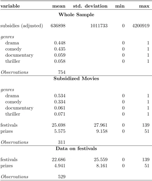
Table 3.1 shows descriptive statistics of the sample. Of the total 754 movies, a sub-sample of 311 was granted public subsidizes from MiBACT to promote relevant cultural aspects of a movie or the work of new directors5_{. Over the}

period under analysis the average public financing per movie was 636 thou-sands of euros with a maximum at 4.2M.

The whole sample shows a strong predominance of dramas and comedies against thrillers and documentaries, with the first accounting for 45% of the sample and the latter for 43%. I want to highlight how the shares of comedies and dramas change when we consider the sub-sample of financed movies: drama quota rise to 53%, while comedies drop to 33%. This shift can be explained by multiple concurrent factors regarding comedies: 1) this kind of movies are less likely to contain cultural aspects of public interest; 2) as shown in Bagella and Becchetti (1999) Italian moviegoers exhibit a strong preference for this genre, with box-offices revenues over the mean so that production companies are less prone to seek for public financing and 3) the presence of young directors that make comedy movies and are granted subsidies ensure that the drop is not even steeper.

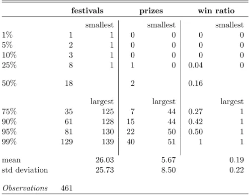
For a sub-sample of 529 motion pictures I got information on the partic-ipation (or not) to film festivals and prizes won at them. 461 movies was exhibited at festivals and were eligible for awards6 _{and 279 of them were}

public financed movies, which account for 90% of the subsidized movies sam-ple. Tables 3.2 and 3.3 highlight some interesting facts in the distribution of these variables. On average each movie in the subset competed in 26 festivals, winning 5.67 prizes. These values slightly rise for financed movies becoming respectively 28.64 participation and 6.21 prizes. For both groups can be seen that there is a predominance of zero awards associated with a pretty low median value (2 for the whole subset and 3 for subsidized movies).

5_{Other than financing movies of particular cultural interest, MiBACT grants financial}

aid to the first or second movie of new directors. The degree of discretion on the allocation of resources from MiBACT to the domestic industry and what can be defined ”cultural interest” is over the scope of this dissertation.

(45)

Table 3.1: Movies Descriptive Statistics

variable mean std. deviation min max Whole Sample subsidies (adjusted) 636898 1011733 0 4200919 genres drama 0.448 0 1 comedy 0.435 0 1 documentary 0.059 0 1 thriller 0.058 0 1 Observations 754 Subsidized Movies genres drama 0.534 0 1 comedy 0.334 0 1 documentary 0.061 0 1 thriller 0.071 0 1 festivals 25.698 27.961 0 139 prizes 5.575 9.158 0 51 Observations 311 Data on festivals festivals 22.686 25.559 0 139 prizes 4.941 8.161 0 51 Observations 529

(46)

The analysis of percentiles shows that the distribution of prizes is heavily shifted to the right, meaning that a small amount of movies conquer the majority of awards. The third column of Tables 3.2 and 3.3 show the ratio between prizes and festivals appearances. While a simple correlation analysis of the two variables indicates a strong reciprocity (⇠0.8), it is of particular interest the fact that the mean and median values are attested around 16-19%, from which we can conclude that an heavy participation commitment to festivals doesn’t automatically drives to more awards.

Table 3.2: Festivals and Prizes

festivals prizes win ratio smallest smallest smallest

1% 1 1 0 0 0 0

5% 2 1 0 0 0 0

10% 3 1 0 0 0 0

25% 8 1 1 0 0.04 0

50% 18 2 0.16

largest largest largest

75% 35 125 7 44 0.27 1 90% 61 128 15 44 0.42 1 95% 81 130 22 50 0.50 1 99% 129 139 40 51 1 1 mean 26.03 5.67 0.19 std deviation 25.73 8.50 0.22 Observations 461

(47)

Table 3.3: Festivals and Prizes – subsidized movies

festivals prizes win ratio smallest smallest smallest

1% 1 1 0 0 0 0

5% 2 1 0 0 0 0

10% 4 1 0 0 0 0

25% 9 1 1 0 0.05 0

50% 20 3 0.15

largest largest largest

75% 39 125 7 44 0.25 1 90% 72 128 16 44 0.40 1 95% 92 130 33 50 0.47 1 99% 128 139 44 51 1 1 mean 28.64 6.21 0.19 std deviation 28.05 9.46 0.23 Observations 279

(48)

3.3 Methodology

Econometric procedures involved in my analysis of the Italian movie industry are pretty straightforward and include Ordinary Least Squares for the study of box-office revenues and the implementation of a count data model when looking at the quality aspect of prizes won by movies. The next section covers in details the theory behind the most used approach when dealing with count variables, the Poisson regression model.

3.3.1 The Poisson regression model

Many economic studies relay on variables that are non-negative integers. Examples includes data on patents granted to firms, number of contacts for call centers or visits to the hospital by an individual. On the same fashion, to analyze the impact of public subsidization on the quality of a film, I will study the prizes won by a movie at film festivals. Data of this type are called count data and the empirical analysis of them is based on models of events. In principle, the study could be done implementing multiple linear regression; however, the preponderance of zeros and small values in the dependent variable and its discrete nature, suggest that it is possible to improve using a di↵erent methodology. Another option that naturally comes to mind is to implement an ordered discrete choice model, like ordered probit. However, this is not usually feasible, because this kind of model requires the number of possible outcomes to be fixed and known.

Concerning the dataset under analysis, from tables 2.1 and 2.2 we can recall that the dependent variable on prizes assume values from 0 to 51 with a strong presence of zeros. To deal with these characteristics we need a model for which any non-negative integer value is a valid, although possibly very unlikely, value. We then first turn to a distribution which has this propriety: the Poisson distribution. Named after French mathematician Sim´eon Denis Poisson, is a discrete probability distribution that expresses the probability of a given number of events occurring in a fixed interval of time and or space if these events occur with a known average rate and independently of the time since the last event.

(49)

If a discrete random variable Y follows the Poisson distribution, then

P rob(Y = y) = e

y

y! , y = 0, 1, 2, ...

Similarly the poisson regression model specifies that each yi is drawn from a

Poisson distribution with parameter i, which is related to the regressors xi.

The primary equation of the model then is

P rob(Y = y_|xi) =

e y

y! , y = 0, 1, 2, ...

The model, like the distribution, is characterize by a single parameter, . The most common formulation for i is the loglinear model,

ln i = x’i .

The expected number of events per period (per festival, in our sample) is given by E[y_|xi] = V ar[y|xi] = i = ex’i then @E[y_|xi] @xi = i .

The easiest way to estimate the parameters of the model is with maximum likelihood techniques. The log-likelihood function will be

ln L =

n

X

i=1

[ i+ yix’i ln yi!].

The likelihood equation is @ln L @ = n X i=1 (yi i)xi = 0

(50)

and the Hessian matrix is @2_{ln L} @ @ 0 = n X i=1 ixix’i.

Since the Hessian is negative definite for all x and , optimization techniques based on Newton’s Method generally work very well and converge rapidly. Given the estimates, the prediction for observation i is ˆi = exp(x’i ).

Because the conditional mean function is nonlinear and the regression is heteroschedastic, the Poisson model doesn’t produce a counterpart to the R2

typical of linear regression models. An alternative based on the standardized residuals that compares the fit of the model with a restricted version with only the constant term is given by the so called pseudo R2_:

R2_p = 1 Pn i=1 " yi ˆi p ˆ_i # Pn i=1  yi y p y .

Davidson and MacKinnon (2005) points out that ”Although its simplicity makes it attractive, the Poisson regression model is rarely entirely satisfac-tory. In practice, even though it may predict the mean event count accurately, it frequently tends to underpredict the frequency of zeros and large counts, because the variance of the actual data is larger than the variance predicted by the Poisson model. This failure of the model is called overdispersion”. As we will see in the next section, I perform a robustness check treating available data with an alternative model: negative binomial. The result of Likelihood ratio test suggests that the model of choice should be the Poisson.

3.4 Estimation Results

As stated in the previous sections, my study of the Italian movie industry resolve around two dimensions: quantity (box-offices revenues) and quality (prizes won at film festivals). For the analysis of box-office performance the

(51)

baseline specification explain the revenue of a movie i (in logs and adjusted for inflation as usual) as a function of subsidization in log form if any and genres: comedy, drama and thriller, with documentary omitted and taken as reference category. The following model is considered:

ln revenuei = 0+ 1ln subsidizationi+ 2comedyi

+ 3dramai+ 4thrilleri+ "i

where r for r = [1, 4] are parameters of the model and ✏i is an error term.

The sample amount to 754 Italian movies exhibited in the domestic market during the 2002-2011 period. I evaluate data with the typical OLS approach, grouping observations by year and comparing results for random and fixed e↵ects models. The random e↵ects assumption is that the individual spe-cific e↵ects are uncorrelated with the independent variables. The fixed e↵ect assumption is that the individual specific e↵ect is correlated with the in-dependent variables. If the random e↵ects assumption holds, the random e↵ects model is more efficient than the fixed e↵ects model. To establish which model fits the data I then perform the Hausman’s (1978)7 _{test, which}

evaluates the consistency of an estimator when compared to an alternative, less efficient, estimator which is already known to be consistent. in other words, helps to evaluate if a statistical model corresponds to the data. In the contest of Panel data, the Hausman test can be used to di↵erentiate between fixed e↵ects and random e↵ects models. Running the test on the data under analysis, we can conclude that the random e↵ect model is to be preferred under the null hypothesis due to higher efficiency (should be noted that both specifications are consistent).

Table 3.4 shows estimations results for the given specification. These first results are consistent with the findings of Bagella and Becchetti (1999) in the sense that highlight the crucial role of comedy genre in driving the box-office performance of Italian movies and the irrelevance and slightly negative e↵ect of subsidization. The following step is to evaluate the impact of public

7_Also _called _the _Wu–Hausman _test, _Hausman _{specification} _test, _and