A new void finder based on cosmic dynamics

A

LMA

MATER

STUDIORUM

— UNIVERSITÀ DI

BOLOGNA

SCUOLA DI SCIENZE

Corso di Laurea Magistrale in Astrofisica e Cosmologia Dipartimento di Fisica e Astronomia

A new void finder based on cosmic dynamics

Tesi di Laurea Magistrale

Candidato:

Carlo Cannarozzo

Relatore: Chiar.mo Prof. Lauro Moscardini

Co-relatore:

Dr. Federico Marulli

Sessione III

Ai miei genitori, Ettore e Maria Rita. A mia sorella, Marcella.

Alla mia ragazza e collega, Matilde.

Allo Zio. “...‘sti vuoti l’ama a ìnghiri!”

Once when Einstein was in Hollywood on a visit Chaplin drove him through the town. As the people on the sidewalks recognized two of their greatest, if very different, contemporaries, they gave them a tremendous reception which greatly astonished Einstein. “They’re cheering us both,” said Chaplin: “you because nobody understands you, and me because everybody understands me.” There was a good-humoured pride in his remark, and at the same time a certain humility as at a recognition of the difference between ready popularity and lasting greatness.

T

ABLE OF

C

ONTENTS

Page Abstract v Sommario ix 1 Introduction 1 2 A Cosmological Background 7

2.1 Fundamentals of General Relativity . . . 7

2.2 The Friedmann–Lemaître–Robertson–Walker Metric. . . 9

2.2.1 The Spatial Curvature . . . 10

2.3 The Hubble Law . . . 12

2.3.1 The Redshift . . . 14

2.4 The Friedmann Equations . . . 15

2.4.1 The Friedmann Models and the Cosmological Constant . . . 15

2.4.1.1 The Big Bang Singularity . . . 18

2.4.2 Flat, Open and Closed Models . . . 19

2.5 TheΛCDM Universe . . . 21

2.6 Gravitational Jeans Instability . . . 23

2.6.1 The Jeans Instability in a Static Universe . . . 24

2.6.2 The Jeans Instability in an Expanding Universe . . . 25

2.6.3 The Linear Regime Theory . . . 27

2.6.3.1 Mass Scales and Filtering . . . 28

2.6.4 Towards the Non-Linear Evolution . . . 29

2.6.4.1 The Zel’dovich Approximation. . . 30

2.7 N-body Simulations . . . 30

3.1 The Historical Discovery of Voids . . . 34

3.2 Voids in aΛCDM Scenario . . . 34

3.2.1 The Role of Voids . . . 35

3.2.1.1 The Importance of Dark Energy . . . 35

3.2.1.2 Passive Evolution of Galaxies within Voids . . . 36

3.2.1.3 The Void Phenomenon . . . 37

3.2.1.4 The Impact on the Cosmic Microwave Background . . . . 38

3.2.1.5 The Alcock-Paczynski Test. . . 38

3.3 Void Morphology . . . 39

3.4 Formation and Evolution of Voids. . . 40

3.5 Void Dynamics . . . 41

3.5.1 From Aspherical to Spherical Shapes . . . 42

4 Looking for Cosmic Voids 45 4.1 Three Categories of Void Finders . . . 45

4.2 Some Specific Void Finder Algorithms . . . 47

4.2.1 Patiri’s Geometrical Void Detection . . . 47

4.2.2 Void Detection in VIPERS. . . 47

4.2.3 The Colberg’s Void Finding Algorithm . . . 49

4.2.3.1 Method . . . 49

4.2.3.2 Results . . . 49

4.2.4 WVF - Watershed DFTE . . . 50

4.2.4.1 Method . . . 50

4.2.4.2 Results . . . 52

4.2.5 ZOBOV & VIDE. . . 53

4.2.5.1 The ZOBOV Method . . . 53

4.2.5.2 Results . . . 54

4.2.5.3 VIDE . . . 54

4.2.6 DIVA . . . 56

4.2.6.1 Method . . . 56

4.2.6.2 Results . . . 57

4.2.7 UVF & LZVF Algorithms . . . 58

4.2.7.1 Method . . . 59

4.2.7.2 Results . . . 60

TABLE OF CONTENTS

4.3.1 The Comparison. . . 61

5 A New Void Finder 63 5.1 The CosmoBolognaLib . . . 63

5.2 The Void Finder Algorithm. . . 64

5.3 The Displacement Field Reconstruction . . . 66

5.3.1 The Theoretical Background . . . 67

5.3.2 The LaZeVo Reconstruction Algorithm . . . 67

5.3.2.1 The Algorithm . . . 67

5.3.3 The RIVA Reconstruction Algorithm . . . 69

5.3.3.1 The Algorithm . . . 70

5.4 The Reconstruction of Divergence Field . . . 70

5.5 The Identification of Cosmic Voids . . . 71

5.5.1 The Void Centre . . . 73

6 Testing the New Void Finder on N-body Simulations 75 6.1 Setting the Initial Parameters. . . 75

6.2 The Displacement Field Maps . . . 76

6.3 The Void Catalogue . . . 78

6.3.1 Void Shapes . . . 79

6.4 Stacked Density Profiles . . . 81

6.5 Comparison with the LZVF Algorithm. . . 84

6.6 Towards a Cosmological Exploitation . . . 93

6.6.1 The Void Size Function . . . 93

6.6.2 The Cleaning Correction. . . 94

6.6.3 Comparing to Theoretical Predictions. . . 95

6.6.3.1 The DM Halo Catalogue . . . 95

6.6.3.2 The Void Catalogue . . . 95

7 Discussion and Conclusions 97 7.1 Our Project . . . 97

7.2 Results. . . 98

7.3 Work in Progress & Future Perspectives . . . 99

A

BSTRACT

C

osmic voids are large empty regions of the Universe, having a huge range in size, from the so-called minivoids, with diameters around 3 Mpc, to supervoids, with diameters of few hundreds of Mpc. Voids separate filaments, sheets and haloes from each other, as predicted by numerical simulations in the framework of the Cold Dark Matter (CDM) models and confirmed by observations. They constitute a fundamental component of the Cosmic Web, accounting for about the 95% of the overall volume of the Universe. Cosmic voids point out the scale at which density fluctuations have decoupled from the Hubble flow and formed overdense regions, such as galaxy clusters (van de Weygaert and Platen,2011). Because of their low-density nature, voids are powerful probes to underline several crucial aspects of the Universe. Indeed, their internal structures, shapes and other statistical properties such as number counts, clustering, density profiles and also their dynamics are supposed to be strongly dependent on Dark Energy (DE) properties. This implies that cosmic voids can be considered as laboratories for testing cosmological models and, in particular, to put constraints on DE and on the geometry of the Universe. Voids are formed from underdensities in the primordial field of density perturbations and, like clusters, may provide crucial information on the large scale structures. In addition, their underdense environment represents the ideal location to study galaxies in passive evolution, to investigate internal feedback phenomena in an environment where galaxy interactions are highly unlikely. On the other hand, precisely because of that pristine low-density environment, void sampling is not trivial. Indeed, Void Finders based on density, or even geometrical, criteria, generally suffer from significant shot noise uncertainties.

In this context, the main goal of this thesis is to implement a new Void Finder code based on a dynamical criterion, following the approach suggested byElyiv et al. (2015). The method aims at sampling cosmic voids in Lagrangian coordinates, thus mitigating the uncertainties due to sparse sampling. The idea is to use tracers as test particles, reconstructing their orbits from the actual clustered configuration to a homogeneous and isotropic pristine distribution. This back-in-time evolution in the

displacement field can be performed adopting two different approaches. The first assumes the Zel’dovich approximation (Zel’dovich,1970). In brief, the linear theory of density perturbations is applicable to a regime in which the density contrast,δρ/ρ, is lower than unity. In the Lagrangian description of a cosmological fluid, one traces the path of a fluid element onto space and time. Given the position q of an element at t0, its location at subsequent instants can be expressed in terms of the Lagrangian displacement field Ψ. This approximation allows to extend the linear theory to the case of perturbations slightly larger than unity. Since objects have straight orbits in this approximation, in order to compute the displacement field we connect their Eulerian positions to those of a randomly distributed sample.

The second approach exploits the two-point correlation function,ξ(r), that quantifies the clustering of a galaxy sample. It represents the excess in probability, dP, compared to that expected in a random distribution, of finding a pair of galaxies separated by a comoving distance r, in the two comoving volume elements dV1 and dV2. Although the local Universe is highly inhomogeneous, in an early epoch the space is supposed to be extremely homogeneous. This suggests that a practical way to trace galaxy orbits back in time is to relax their present spatial distribution to homogeneity, defined as a state in which the correlation function at all separations is zero.

Since, in both the approaches described above, the particle path depends on the initial random seeds, our Void Finder algorithm performs several reconstructions and then averages the obtained fields by using a Gaussian weighting. Then it computes the divergence field,Θ= ∇ ·Ψ, that represents, by definition, the density at each point. We consider only the local minima with negative divergence. Each local minimum identifies a subvoid. In fact, a negative value of velocity field divergence implies the presence of a region acting as a sink of mass streamlines. Through a watershed method we can then “fill” the near subvoids in order to identify, eventually, a local void. The void centres are assumed to be the positions corresponding to the absolute minimum value of the divergence field inside each void. To estimate the void size, we calculate the effective radius of an equivalent spherical volume.

The new dynamical Void Finder implemented in this work has been included in the

CosmoBolognaLib, a large set of Open Source C++/Pythonlibraries for cosmological calculations (Marulli et al., 2016). In order to check the robustness of our new Void Finder, we compared this code to the LZVF algorithm (Elyiv et al., 2015), finding a good agreement in the detection of voids. In the next future, we will extend this work, applying our algorithm to observed datasets, such as the VIPERS catalogues (Guzzo

and The Vipers Team,2013). The following step will be to include our Void Finder in a statistical numerical pipeline to be used to extract cosmological constraints from void number counts and clustering, and to study the ellipticity of cosmic voids.

Our Void Finder is currently competing in the new Void Challenge, that is being carried on to prepare the scientific exploration of theEuclidspace mission (Laureijs et al., 2011), whose primary goal is to compare different methods to detect cosmic voids.

S

OMMARIO

I

vuoti cosmici sono ampie regioni sottodense dell’Universo, le cui dimensioni variano dai cosiddetti minivoids, il cui diametro è di qualche Mpc, fino ai supervoids, con diametri dell’ordine delle centinaia di Mpc. I vuoti separano i filamenti e gli aloni di Materia Oscura tra loro, come previsto da simulazioni numeriche di modelli di Materia Oscura Fredda, confermati ulteriormente dalle osservazioni. I vuoti rappresentano una componente fondamentale della Rete Cosmica, occupando circa il 95% del volume totale dell’Universo. Queste strutture demarcano la scala alla quale le fluttuazioni del campo di densità si disaccoppiarono dal flusso di Hubble, andando a costituire regioni sovradense, come ad esempio gli ammassi di galassie (van de Weygaert and Platen,2011). A causa della loro natura sottodensa, i vuoti rappresentano un importante mezzo per l’indagine di molti aspetti cruciali dell’Universo. Infatti, la loro struttura interna ed altre proprietà statistiche, come ad esempio i conteggi, i profili di densità ed anche la dinamica sono fortemente influenzati dalla presenza dell’Energia Oscura. Ciò implica che queste strutture possano essere considerate come dei laboratori nei quali testare i modelli cosmologici ed, in particolare, essere utili per porre alcuni vincoli sull’Energia Oscura e sulla geometria dell’Universo. Come gli ammassi di galassie, anche i vuoti possono fornire informazioni cruciali riguardanti la struttura su larga scala dell’Universo. Inoltre, il loro ambiente notevolmente sottodenso rappresenta il luogo ideale all’interno del quale le galassie possono evolvere passivamente, senza risentire di alcuna interazione esterna. Ciò consente quindi di poter investigare gli aspetti evolutivi interni delle galassie, in un ambiente in cui le interazioni esterne sono altamente improbabili. Tuttavia, proprio a causa della scarsa densità in questi ambienti, la loro identificazione non è affatto banale. Negli anni, infatti, molti algoritmi sono stati sviluppati per la ricerca dei vuoti cosmici. Alcuni di questi codici, basandosi su criteri di densità o di geometria, sono fortemente soggetti al campionamento delle sorgenti utilizzate per la ricerca dei vuoti. In questo quadro generale, lo scopo principale di questo progetto di tesi è stato quindi l’implementazione di un nuovo codice per la ricerca dei vuoti basato su criteri dinamici, seguendo l’approccio proposto da Elyiv et al.(2015). L’idea

di base consiste nell’impiegare i traccianti come particelle di prova, ricostruendo le loro orbite a partire dalla configurazione attuale fino al raggiungimento di una distribuzione omogenea ed isotropa dell’Universo. Questa evoluzione all’indietro nel tempo del campo di spostamento dei traccianti può essere eseguita utilizzando due diversi metodi. Il primo metodo si avvale dell’approssimazione di Zel’dovich. Sostanzialmente, la teoria lineare delle perturbazioni di densità è applicabile ad un regime in cui il contrasto di densità,δρ/ ¯ρ, è minore di uno. Nella descrizione Lagrangiana di fluido cosmologico, si può tracciare il percorso di un elemento di fluido nello spazio e nel tempo. Data una posizione q di un elemento di fluido all’istante t₀, la sua posizione agli istanti successivi può essere espressa in termini del campo di spostamento Lagrangiano,Ψ. Questa approssimazione consente, perciò, di estendere la teoria lineare delle perturbazioni di densità poco al di sopra dell’unità. Poiché le orbite percorse dagli oggetti sono lineari, per ricostruire il campo di spostamento Lagrangiano basta connettere le posizioni Euleriane dei traccianti a quelle di una distribuzione casuale.

Il secondo approccio sfrutta invece le proprietà della funzione di correlazione a due punti,ξ(r), che rappresenta l’eccesso di probabilità, dP, rispetto a quella attesa in una distribuzione casuale, di trovare una coppia di galassie ad una distanza comovente r, nei rispettivi elementi di volume comoventi, dV1 e dV2. Sebbene l’Universo locale è altamente disomogeneo, si ipotizza che, in un’epoca primordiale, l’Universo fosse stato caratterizzato da una distribuzione omogenea. Per questo motivo, un valido metodo per tracciare l’orbita delle galassie indietro nel tempo consiste proprio nel rilassare la distribuzione spaziale attuale fino al raggiungimento dell’omogeneità, quest’ultima caratterizzata da una funzione di correlazione ovunque nulla.

Dal momento che in entrambi gli approcci descritti il cammino percorso da una particella dipende dalla configurazione casuale iniziale, il nostro algoritmo esegue diverse ricostruzioni del campo di spostamento, successivamente mediate tra loro, introducendo un peso Gaussiano. Successivamente, viene calcolato il campo di divergenza,Θ= ∇·Ψ, che rappresenta, per definizione, la densità in ogni punto. Ogni minimo locale identificherà così una regione sottodensa, detta subvoid. Attraverso la tecnica watershed, le regioni sottodense vicine identificheranno un unico vuoto locale. I centri dei vuoti saranno quindi definiti come i minimi assoluti del campo di divergenza all’interno di ogni vuoto. Per fornire una stima delle dimensioni dei vuoti cosmici identificati, viene calcolato il raggio effettivo, ossia il raggio di una sfera avente pari volume del vuoto considerato.

Il nostro metodo dinamico di ricerca dei vuoti cosmici è stato incluso nelle librerie

robustezza del nostro nuovo algoritmo, abbiamo effettuato una comparazione diretta con il metodoLZVFproposto daElyiv et al.(2015). Da questo confronto, abbiamo avuto un ottimo riscontro riguardante i vuoti identificati da entrambi i metodi. Abbiamo intenzione prossimamente di estendere l’impiego del nostro algoritmo su campioni di dati osservativi, come ad esempio i cataloghi VIPERS (Guzzo and The Vipers Team, 2013). Il passo successivo sarà quello di utilizzare questo algoritmo per estrarre vincoli cosmologici, a partire dai conteggi dei vuoti cosmici a studiarne la loro ellitticità.

Infine, il nostro metodo sta attualmente competendo nell’ambito della nuova Void Challenge, una competizione inerente alla preparazione della missione spazialeEuclid

(Laureijs et al., 2011), il cui principale scopo è il confronto tra metodi differenti per identificare i vuoti cosmici.

C

H A P T E R

1

I

NTRODUCTION

T

he ΛCDM Cosmological Model, also called the Standard Cosmological Model, can be directly constructed from the Einstein’s Field Equations, assuming the Cosmological Principle, i.e. the conditions of homogeneity and isotropy in the entire Universe, adding the further contribution of the Cosmological Constant,Λ. This theoretical model is constrained by a set of cosmological parameters, describing the energy content, principally due to the Cold Dark Matter and the Dark Energy. There are some still unsolved issues related to the Standard Cosmological Model, such as the intrinsic nature of Dark Matter and Dark Energy. Indeed, although the presence of the Cosmological Constant,Λ, provides an accurate description of the current accelerated expansion of the Universe, it does not provide information about the acting trigger mechanism.

The Large Scale Structure of the Universe, can be exploited to put constraints on all the parameters of the cosmological model. For instance, we can perform measurements of the matter perturbations, deviating from the assumption of the Cosmological Principle, by the smallness of the CMB anisotropies (_{δT/ ¯T ≈ 10}−5_{), on analysing wide galaxy} redshift surveys, in order to describe the lower wavenumbers k of the power spectrum. The study of the the largest and most extreme structures in the mildly non-linear regime allows us to extend our knowledge of the Universe.

The Cosmological Principle is drastically violated at small scales, due to the growth of primordial perturbations in the matter density distribution of the Universe. In the earliest phases of the evolution of the Universe, the radiation and matter components

were coupled via the Thomson scattering. The fluctuations in the temperature spectrum generated anisotropies, and hence the inhomogeneous distribution of the density field. The following structure formation is the result of the gravitational instability acting on those perturbations of matter. The fluctuation distribution can be represented, in a first approximation, as a Gaussian random field. Thanks to the gravitational force, the perturbation amplitudes started to grow, eventually causing collapse. The overdense regions increased their density contrast,δ, while the cosmic depressions in the density field decreased their δ. As a consequence, the increasing of density in some zones pro-duced an even stronger gravitational field. On the contrary, in the regions characterised byδ < 0, the gravitational force became weaker than the mean value. So, the self-gravity reduced its effect, implying that the expansion decelerated less than the rest. In this scenario, the underdensities started to expand faster than the Hubble flow.

The formation and evolution of the cosmic structures generated the so-called Cosmic Web, as predicted in the framework of the CDM cosmology (Bond et al.,1998). The result of the gravitational anisotropic collapse is the formation of Dark Matter haloes, filaments, sheets, walls and large areas empty of matter, the so-called cosmic voids. Galaxies, following the Dark Matter distribution, were arranged in galaxy clusters, surrounded by a filamentary frame, the latter drawing the void boundaries. As a consequence of their underdensities, the void dynamics is mainly dominated by the Dark Energy. The presence of the Cosmic Web has been confirmed in all large redshift surveys (e.g.,Alam et al.,2015;Guzzo and The Vipers Team,2013;Colless et al.,2003;de Lapparent et al., 1986).

Cosmic voids emerged out of the density depressions of the Universe on the primordial fluctuation field. The presence of cosmic voids in the LSS distribution is one of the most important and earliest prediction of the CDM model (Hausman et al., 1983). Since their discovery (Gregory and Thompson,1978;Jõeveer et al.,1978), cosmic voids have represented an important brick in the modern cosmological framework. The drastic change in the concept of the large scale structure of the Universe, due to the void discovery, has been carried out thanks to the realisation of several wide-angle and deep galaxy redshift surveys.

Though a widespread and unique definition of cosmic void has not yet been provided, we now have a coherent picture about the main void properties in theΛCDM cosmo-logical model. In this scenario, voids are underdense regions placed anywhere in the Universe, accounting for the 90 − 95% of the entire volume (Platen et al.,2007). In a first approximation, we may consider voids as large spherical volumes, spanning a wide range

of scales, from the so-called minivoids (few Mpc in radii) (Tikhonov and Karachentsev, 2006), to the giant supervoids, with radii of around one hundreds of Mpc, as theCold Spotin the CMB (Szapudi et al.,2014).

As already mentioned, cosmic voids can play a fundamental role in providing con-straints on the Dark Energy (e.g.,Granett et al.,2008), and are the ideal sites where to study modified gravity (e.g., Li et al., 2015). Indeed, several investigations can be performed with cosmic voids: through weak gravitational lensing (e.g.,Sánchez et al., 2017;Clampitt and Jain,2015), estimating the Integrated Sachs-Wolfe effect (e.g.,Planck Collaboration et al.,2016;Cai et al.,2014), investigating the Dark Matter nature (e.g., Yang et al.,2015), studying the void ellipticity caused by the action of Dark Energy (e.g., Pisani et al.,2015;Sutter et al.,2015a), constraining the Universe geometry through the Alcock-Paczy ´nski test (e.g.,Sutter et al.,2014b;Lavaux and Wandelt,2012), revealing the baryon acoustic oscillations (e.g.,Kitaura et al.,2016), testing coupled Dark Energy models (e.g.,Pollina et al.,2016), providing void size abundances and stacked density profiles for gravitational theories (e.g.,Zivick et al.,2015;Cai et al.,2015), testing evolu-tion models of isolated galaxies, thanks to their pristine environment (e.g.,Penny et al., 2015), and much more.

One of the most tricky issues about voids concerns the non-general concordance of their definitions. During the last years, several algorithms able to identify the cosmic voids have been proposed.Lavaux and Wandelt(2010) classified the different Void Finder Algorithms into three broad classes.

The first category is based on a density criterion (e.g.,Micheletti et al.,2014;Elyiv et al.,2013;Patiri et al.,2006;Hoyle and Vogeley,2002;El-Ad et al.,1997). Void Finders belonging to the first class define cosmic voids as volumes with no tracers within, or with a local density value lower than the mean density of the Universe.

The second class refers to the Void Finders that identify voids following a geometrical approach, by using, for instance, polyedra, spheres or tessellations (e.g., Sutter et al., 2015b;Neyrinck,2008;Platen et al.,2007;Colberg et al.,2005).

Finally, the third class includes the algorithms which detect voids using dynamical criteria. In this case, the tracers (e.g., galaxies) are considered as test particles able to identify “unstable” points in the density field (e.g., Elyiv et al., 2015;Lavaux and Wandelt,2010;Hahn et al.,2009).

The first two categories of Void Finder algorithms detect cosmic voids using the Eulerian positions of the tracers. These approaches, however, are subject to various problems. When using mass tracers for the reconstruction of the density distribution, a

bias prescription has to be taken into account. The importance of the bias modelling has been discussed inPollina et al.(2016), in particular to discriminate between different cosmological models. Another drawback is due to the definition of voids as underdensities. Indeed, Eulerian-position algorithms are strongly prone to the shot-noise error. On the contrary, the algorithms of the third-class, which rely on the Lagrangian positions, suffer less the shot-noise problem.

The main goal of this thesis work is the development of a new Void Finder algorithm based on a dynamical criterion, able to identify the depressions in the density field. This algorithm is composed by three main steps. The first step deals with the reconstruction of the displacement field of the tracers, the latter used as test particles, in a back-in-time evolution. This reconstruction can be performed by two different methods,LaZeVo, exploiting the Zel’dovich approximation, andRIVA, which relies on the measurement of the two-point correlation function. Once the displacement field has been reconstructed, the second step computes the divergence of the velocity field, which represents, by definition, the density field. Since voids are defined as regions of negative velocity divergence, the second step looks for the density local minima, as cosmic voids candidates. By performing a filling of the depressions in the density field, through the watershed technique, the third steps identifies the cosmic voids.

This new Void Finder is now part of theCBLproject (Marulli et al.,2016), a set of

C++/Pythonlibraries for cosmological calculations.

We propose an application of our Void Finder to a DM halo catalogue, making also a direct comparison with an already existing algorithm, i.e. theLZVFmethod proposed by Elyiv et al.(2015).

Then, we discuss the first results obtained in the context of the newVoid Challenge, proposed inside theEuclidspace mission collaboration, whose aim consists in a compari-son between different methods for the identification of cosmic voids.

This thesis work is organised as follows:

• Chapter 2 deals with an overview of the cosmological framework, introducing the theoretical basis of the Standard Cosmological Model;

• Chapter 3 illustrates the role of the cosmic voids in the Universe, reviewing some studies concerning their structure, formation, evolution and dynamics;

• Chapter 4 provides a general overview about the Void Finders, subdivided according to the criterion used to detect cosmic voids;

• Chapter 5 accurately describes the internal structure of our new Void Finder, ex-plaining the methods used to reconstruct the displacement field and its divergence and the identification of voids;

• Chapter 6 deals with the main results obtained by applying our new Void Finder to a DM halo catalogue, comparing them to those of theLZVFalgorithm; moreover, we present a first application of our method in the context of the newEuclid Void Challenge;

• Chapter 7 summarises the results of this project, focusing on the possible future perspectives.

C

H A P T E R

2

A C

OSMOLOGICAL

B

ACKGROUND

I

n this chapter we summarise briefly the cosmological framework on which this thesis work is based. We provide the main equations which are the basis of the theoretical models, describing the growing and the dynamical evolution of the Universe. Insection 2.1we start by introducing some notions about General Relativity and in particular the Einstein’s Field Equations. In section 2.2 we define the Fried-mann–Lemaître–Robertson–Walker metric, that describes the curvature of the spatial hypersurfaces of the Universe. In section 2.3we introduce the Hubble Law and the definition of Redshift. In section 2.4 we illustrate the Friedmann Equations, as the solutions to the Einstein’s Field Equations and we make a comparison between the three possible geometrical models. Insection 2.5we illustrate the main features of the Standard Cosmological Model. Thesection 2.6deals with the Jeans theory about the model gravitational instability and we discuss the growth of the primordial fluctuations in the linear regime and beyond.

2.1

F

UNDAMENTALS OF

G

ENERAL

R

ELATIVITY

Gravity is expected to be the main force acting throughout the Universe on large scales. The best description of this force is given by the Theory of General Relativity (GR) proposed by Albert Einstein in 1915 (Einstein,1915).

In this context, the geometry of space-time is described by the metric tensor, g_µν. The invariant interval between two different events in space-time, (t, x1, x2, x3) and

(t0, x0₁, x0₂, x0₃) = (t + δt, x1+ δx1, x2+ δx2, x3+ δx3) is defined by

(2.1) ds2= gµνdxµdxν.

This interval can be explicitly separated out as

(2.2) ds2= g00dt2+ 2g0idxidt + gi jdxidxj,

where g00dt2 is the time component, gi jdxidxjthe spatial components and 2g0idxidt the mixed components. By defining the Riemann tensor as follows

(2.3) R_αβγµ ≡dΓ µ αγ dxβ − dΓµ_αβ dxγ +Γ µ σβΓσγα−ΓµσγΓσβα,

in which Γ·_·· are the terms of the affine connection, Rµ_αβγ is a fourth-order tensor con-tractible to the Ricci tensor, Rµν, or further to the curvature scalar, R:

(2.4) R_αβ≡ Rµ_αβµ, R ≡ Rµµ= gµνRµν.

We introduce the energy-momentum tensor, T_µν, which describes the content of energy and matter in the Universe. We can connect T_µνwith the space-time metric by using the Einstein’s Field Equations:

(2.5) R_µν−1

2gµνR = 8πG

c4 Tµν,

where G and c are the gravitational constant and the speed of light, respectively. Looking at the left-hand side of the equation (2.5), we can define the Einstein tensor G_µνas

(2.6) G_{µν≡ Rµν−}1

2gµνR.

This tensor has zero covariant divergence, according to what we want to obtain for T_µν by virtue of the conservation laws. Combining the equations (2.5) and (2.6), we obtain the final formula of the Einstein’s gravitational field equations:

(2.7) G_µν=8πG

c4 Tµν.

We will consider a set of homogeneous and isotropic models. First of all, if the mean free path of particles constituting a fluid, _λm f p, is lower than the physical scales of interaction, we may consider this fluid as perfect. The different energy components in a Big-Bang model description constitute the so-called perfect fluid. Considering this perfect fluid in its rest-frame, the related energy-momentum tensor T_µνcan be written as follows:

(2.8) T_{µν= −p gµν+ (p + ρc}2) u_µu_ν,

where p is the pressure term,ρc2 is the energy density term and u_· are the components of the 4-velocity of the fluid element.

2.2. THE FRIEDMANN–LEMAÎTRE–ROBERTSON–WALKER METRIC

2.2

T

HE

F

RIEDMANN

–L

EMAÎTRE

–R

OBERTSON

–W

ALKER

M

ETRIC

In order to describe the Large Scale Structure (LSS), we can assume the Cosmological Principle (CP) that asserts that there are no observable inhomogeneities at large scales. Hence, the Universe appears to be homogeneous and isotropic. Homogeneity implies that all observers, in different places all around the Universe, observe the same properties, while isotropy involves that there are not favourite directions. Having established the concept of the CP, our goal is to see if it is possible to construct some models of the Universe in which this principle is satisfied. Hence, the task is to find solutions to the Einstein’s Field Equations.

Assuming homogeneity and isotropy, we can define a universal time such that the spatial metric is the same in each point at all times. The isotropy, for which there are no preferential directions in the Universe, implies that the mixed components, g0i, of the equation (2.2) have to be null. Thus we can obtain the following form of the metric:

(2.9) ds2= c2dt2− gi jdxidxj= c2dt2− dl2.

As already expressed in the previous section, we can regard the Universe as a continuous fluid in which each element is marked with a set of three spatial coordinates xi _{(with i = 1, 2, 3). Furthermore, we define a proper time, that is measured by a clock} moving with the perfect fluid.

The geometrical properties of the space-time are described by a metric. By using the time coordinate (the first term on the right-hand side of the equation (2.9)) and assuming the spatial isotropy, we can derive the most general form of the equation (2.9) that verifies the CP as follows:

(2.10) ds2= c2dt2− a2(t) · dr2 1 − κr2+ r 2_(sin2_{θ dϕ}2 + dθ2) ¸ .

The formula (2.10) defines the Friedmann–Lemaître–Robertson–Walker (FLRW) metric expressed in spherical polar coordinates, where r,θ and ϕ are the dimensionless comov-ing coordinates and t is the proper time. In this metric also two new terms appear: a(t) is the cosmic scale factor (or the expansion parameter), having the dimensions of a length, andκ is the curvature parameter. The value of κ and the function a(t) can be derived by the Einstein’s Field Equations, for any given energy-momentum tensor.

Let us consider a free massive particle at rest located at the origin of the comoving system at an instant in time. The absence of preferred directions ensures that no velocity variation can be induced on this particle by gravity. Thanks to the required homogeneity, the world lines xi= const are the so-called geodesics.

2.2.1 THESPATIALCURVATURE

The curvature of the spatial hypersurfaces of the Universe can be positive, zero or negative. Indeed, the curvature of the space-time depends on the value of the parameter κ, which can be scaled in such a way that the only three possible values are +1, 0 or -1.

To figure out what the scale factor a(t) really is, we can calculate the proper distance at time t from the origin to a comoving particle at radial coordinate r. It is convenient to introduce a coordinateχ defined as

(2.11) χ ≡

Z _dr

p

1 − κr2.

By introducing the three possible values of_{κ in the equation (}2.11), we obtain

(2.12) χ =            sin−1r forκ = +1 r forκ = 0 sinh−1r forκ = −1 or rewriting in terms of (χ, θ, ϕ), the FLRW becomes

(2.13) dl2= a2[dχ2+ f2(χ)(dθ2+ sin2θ dϕ2)], with (2.14) f (χ) =            sin_χ for_{κ = +1} χ forκ = 0 sinhχ forκ = −1 .

The three values of the curvature parameter lead to three different geometries of the Universe. If κ = 0, the space has an infinite curvature. This is the flat Universe case, where the geometry is Euclidean. Forκ = +1, the properties of the hypersphere are more complex. This is the closed Universe case. The space has a finite volume, but has no boundaries, analogous to the two-dimensional case of a sphere. In this case, the equation (2.13) describes a 3D-sphere with radius a in a four-dimensional flat space. Such a sphere is defined by

2.2. THE FRIEDMANN–LEMAÎTRE–ROBERTSON–WALKER METRIC

Introducing the angular coordinates (χ, θ, φ) we obtain: x1= a cos χ sin θ sin φ, x_{2= a cos χ sin θ cos φ,} x_{3= a cos χ cos θ,} x4= a sin χ. (2.16)

By expressing dxi in terms of polar coordinates in the line element

(2.17) dL2= dx2₁+ dx2₂+ dx2₃+ dx2₄,

the metric takes the same form of the relation (2.13), forκ = +1: (2.18) dL2_{s phere}= a2[dχ2+ sin2χ(dθ2+ sin2θ dφ2)].

The space of the closed Universe is totally covered by the following range of angles

0 ≤ χ < π, 0 ≤ θ < π, 0 ≤ φ < 2π, (2.19)

and the maximum volume is

(2.20) V_max= Z 2π 0 dφ Z π 0 dθ Z π 0 dχ = a3 Z 2π 0 dφ Z π 0 sinθ dθ Z π 0 sin2χdχ = 2π2a3. The surface of a 2D-sphere (withχ = const) is

(2.21) S = 4πa2sin2χ.

This surface has the maximum value forχ = π/2 and it is null for χ = 0, π. In such a space the surface S is larger than in flat geometry and the sum of internal angles of a triangle is greater thanπ.

The third case, forκ = −1, is characterized by a hyperbolic geometry. A 3D-hyperboloid is described by the following relation:

(2.22) − x21− x22− x23+ x24= a2.

Analogously to the spherical case described above, the line element is

We can also define a set of angular coordinates with

x_{1= a sinh χ sin θ sin φ,} x2= a sinh χ sin θ cos φ, x_{3= a sinh χ cos θ,} x_{4= a cosh χ,} (2.24)

so that the line element becomes

(2.25) dL2_{h yperbol oid}= a2[dχ2+ sinh2χ(dθ2+ sin2θ dφ2)].

The properties of a geometrical space having a constant negative curvature are similar to those of a flat case. In fact, it represents an infinite open Universe. The range of coordinates are the following:

0 ≤ χ < ∞, 0 ≤ θ < π, 0 ≤ φ < 2π, (2.26)

and the surface, S, is defined by

(2.27) S = 4πa2sinh2χ.

In this particular case, the sum of the internal angles of a triangle is lower thanπ and the surface is greater than the Euclidean one.

2.3

T

HE

H

UBBLE

L

AW

Let us consider a point P at a distance dP from another point P0. The proper distance, d_P, is defined as the distance measured by observers which connect P to P0at a given time t. From the FLRW metric (eq. (2.10)), for dt = 0, we have

(2.28) d_P= Z r 0 a(t) dr0 p 1 − κr2 = a(t) f (r).

It can be observed that the nonstatic nature of the FLRW metric is due to the time dependence of a(t). At time t, the proper distance is related to the present one (t0) by the following relation:

2.3. THE HUBBLE LAW

where a0≡ a(t = t0). The previous quantity is called the radial comoving distance because it remains the same as the Universe expands. The direct link between the two definitions is the following:

(2.30) d_P=a(t)

a₀ dC.

We can observe from eq. (2.30) that the proper and comoving distances are equal at the present time, t0.

The expansion parameter, a(t), varies over time, and the proper distance, dP, varies as well. This implies the existence of a radial velocity, vr, as derivative of dP with respect to t:

(2.31) v_r=ddP

dt = d

dt[a(t) f (r)] = ˙a (t)f (r) + a(t) ˙f(r).

Because of the time-independence of the f (r) term, the relation (2.31) becomes

(2.32) v_r= ˙a(t) f (r) =a(t)˙ a(t)dP.

The equation (2.32) is the so-called Hubble Law and the relative quantity

(2.33) H(t) ≡a(t)˙

a(t)

is the Hubble parameter. Combining eqs. (2.31) and (2.32), we obtain the direct link between the radial velocity and the proper distance, as follows:

(2.34) v_{r= H(t) dP}.

The Hubble parameter provides information on the isotropic expansion velocity. This parameter is usually called the Hubble constant, erroneously. Though H(t) is actually a function of time, it has the same value across the Universe at a given cosmic time. The most recent estimate of the Hubble constant at the present time, H(t0) ≡ H0, is provided by theSDSS-III Baryon Oscillation Spectroscopic Survey (BOSS)(Grieb et al.,2016), is (2.35) H0= 67.6+0.7_−0.6km s−1Mpc−1.

It is conventional to introduce a dimensionless parameter, h, redefining the Hubble parameter as

(2.36) H0= 100 h km s−1Mpc−1.

The motion of objects due solely to the expansion of the Universe is called the Hubble flow. We can see that H0is expressed in units of s−1: the inverse of the Hubble parameter may provide a rough estimate of the age of the Universe (approximately 14 Gyr).

2.3.1 THEREDSHIFT

The redshift is defined as the relative difference between the observed,λoss, and emitted, λem, wavelengths

(2.37) z ≡λoss− λem

λem ,

or analogously for frequencies, by means of the relationλ = c/ν. From eq. (2.37), we can see that z is a positive quantity when the electromagnetic radiation from an object is increased in wavelength, and so shifted to the red region of the spectrum.

Consider a source emitting a photon with wavelengthλem at time tem. An observer located at a distance d will receive the signal with wavelengthλoss at toss. Photons move along null geodesics during the expansion of the Universe. Hence, the term ds2is equal to zero. From the last assumption and the FLRW metric, one has the following relation:

(2.38) c2dt2− a2(t) µ dr2 p 1 − κr2 + r 2 (dθ2+ sin2θ dϕ2) ¶ = 0.

Let us assumeθ and ϕ constants for simplicity such that, integrating the metric along the path, eq. (2.38) becomes

(2.39) Z toss tem c dt a(t)= Z r 0 dr02 p 1 − κr02 = f (r).

Now let us suppose that a second photon is emitted with a time delay,δtem, with respect to the first one and reaches the observer at t0_oss= toss+ δtoss. Since for the two photons the path is the same ( f (r) does not change because of the assumption of comoving coordinates) and the difference is just in time, we can express eq. (2.39) as

(2.40)

Z t_oss tem

c dt

a(t)= f (r).

If the time intervals are small (δt → 0), we can consider a(t) almost constant and therefore

(2.41) δtoss

a(toss)= δtem a(tem). Sinceδt = 1/ν and λ = c/ν, we obtain

(2.42) 1 + z =aoss

a_em,

or, more generally, for an observer located at present time and a generic instant t, we have

(2.43) 1 + z = a0

a(t).

2.4. THE FRIEDMANN EQUATIONS

2.4

T

HE

F

RIEDMANN

E

QUATIONS

GR describes the relation between the geometry of space-time, represented by the metric tensor g_µν(xi), and the energy content of the Universe, expressed by the energy-momentum tensor T_µν(xi). Without any futher assumption on the geometry of the Universe, we can apply the FLRW metric (eq. (2.10)) to the Einstein Equations (eq. (2.5)). Among the 16 equations of the system, just two are independent. The two solutions, assuming the CP and Perfect Fluid, provide the time evolution of a(t) describing the growth of the Universe. They are called the First and the Second Friedmann Equations and can be expressed as follows:

(2.44) a = −¨ 4π 3 G µ ρ +3p c2 ¶ a, (2.45) a˙2_{+ κc}2₌8π 3 Gρa 2_.

Assuming the Universe as a closed system, unable to lose energy, the two equations above can be linked to each other by the adiabatic condition

(2.46) dU = −pdV ,

whereU is the internal energy of the Universe. Equation (2.46) can also be expressed as follows: (2.47a) d(ρc2a3_{) = −pda}3, (2.47b) pa˙ 3₌ d dt(a 3 (ρc2+ p)), (2.47c) _{ρ + 3}˙ ³_{ρ +} p c2 ´a˙ a= 0.

Each constituent of the Universe has its own equation of state, but all of them contribute to the density termρ.

2.4.1 THEFRIEDMANN MODELS AND THE COSMOLOGICAL CONSTANT

In 1922, the mathematician Alexander Friedmann provided the two solutions of the Ein-stein Equations, implementing a set of cosmological models. At that time, the Universe

was assumed to be static, and hence ¨a = ˙a = 0. However, as we can see from equation (2.44), the Universe can be static if and only if

(2.48) ρ = −3 p

c2.

In other words, either the pressure or the energy density must be negative. A fluid with these characteristics does not seem to be physically acceptable. Since also Einstein was convinced that the Universe was static, he added a new term to the eq. (2.5), modifying the equation as follows:

(2.49) R_µν−1

2gµνR −Λgµν= 8πG

c4 Tµν.

Λ is the so-called Cosmological Constant. As we shall see, an ad hoc choice of Λcan imply a static model. Equation (2.49) is the most general possible modification of the original Einstein Equations, enough to satisfy the condition that T_µνis equal to a tensor constructed only from the metric g_µνand its first and second derivatives.

We can write eq. (2.49) by modifying the energy-momentum tensor, so as to obtain a similar form to the original one

(2.50) R_µν−1

2gµνR = 8πG

c4 Teµν, where the new tensor is formally given by

(2.51) Teµν≡ Tµν+ Λc4 8πGgµν, or equivalently (2.52) Teµν≡ −p g_e µν+ (p +_e ρc_e 2 ) u_µu_ν

with the effective pressure and density

(2.53) p ≡ p −_e Λc

4

8πG, ρ ≡ ρ +e

Λc2 8πG.

When Hubble finally discovered the expansion of the Universe (Hubble,1929), Ein-stein regretted the introduction of Λ. Neverthless,Λ-models have been reintroduced recently to describe the accelerated expansion of the Universe, firstly observed from Supernovae (SNe) (Perlmutter et al.,1999;Schmidt et al.,1998;Riess et al.,1998). The Cosmological Constant has the effect similar to repulsive force that contrasts with the gravitational pull.

2.4. THE FRIEDMANN EQUATIONS

Nowadays, scientists have not yet figured out what Λreally is. The origin of this “push” shall be assigned to the Dark Energy.

We can specify the Equation of State (EoS) for the fluid in the form p = p(ρ). In particular, by introducing the w parameter and assuming no variations in time of the entropy S (adiabatic condition) , the EoS becomes

(2.54) p = wρc2.

The w parameter lies in the so-called Zel’dovich interval:

(2.55) 0 ≤ w < 1.

In the following, we will consider just perfect fluids described by EoS satisfying the condition given by eq. (2.55) and also assuming w = −1 in the case of aΛ-Universe.

The fluid can be in two different states: non-relativistic and relativistic. The first case is represented by dust, having w = 0, i.e. with null pressure. While a non-degenerate and ultra-relativistic fluid has an EoS with w = 1/3. This is the case for a radiative fluid or, more generally, for photons and relativistic particles like neutrinos.

The w parameter is directly related to the adiabatic sound speed of a fluid:

(2.56) c_s=s ∂p ∂ρ ¯ ¯ ¯ ¯ ¯ S .

We can note that w can not go beyond 1, because it would imply a speed of sound greater than c. A peculiar case, out of the range given by eq. (2.55), is w = −1, that describes a perfect fluid with effects equivalent to the ones of the cosmological constant.

By replacing the p term in the left-hand side of the adiabatic condition (eq. (2.47a)) with the right-hand side of the EoS (eq. (2.54)), one can derive how the density evolves in time: (2.57) ρ = ρ0 µ _a a₀ ¶−3(1+w) = ρ0(1 + z)3(1+w).

The density evolution depends on the value of w. This can be used to determine which component dominates over the others at a given redshift.

The Second Friedmann Equation can provide us information about the curvature. Indeed, we can rewrite the equation as follows

(2.58) µ ˙ a a ¶2µ ρ ρc− 1 ¶ =κ c 2 a2 ,

whereρcis the critical density, for which the spatial geometry of the Universe is flat:

(2.59) ρc(t) ≡3H

2_(t) 8πG .

The expansion of the Universe will go on indefinitely ifρ < ρc, while it will be halted and then followed by a contraction ifρ > ρc. We can define the dimensionless density parameter as

(2.60) Ω(t) ≡ ρ(t)ρc(t).

As well as the energy density term represents one or more of the components, theΩ parameter can be composed of one or more contributions. It is greater than, equal to or less than unity if the Universe is closed (κ = +1), flat (κ = 0) or open (κ = −1), respectively. By assuming a cosmological model with a single dominant component, one can re-express eq. (2.57) in terms of the density parameter as follows:

(2.61) Ω−1_w (z) − 1 = Ω

−1 0 − 1 (1 + z)1+3w,

where the dependence on the kind of component (e.g., dust, radiation,Λ) is made explicit. Moreover, it is useful to express the Second Friedmann Equation in term ofΩ, H and z. By combining this equation with the definition of the density parameter, the Hubble Law and the eq. (2.43), we obtain

(2.62) H2_{(z) = H}2_{0(1 + z)}2 Ã 1 −X i Ω0,wi+ X i Ω0,wi(1 + z) 1+3wi ! ,

in which H(z) is the Hubble parameter at a generic redshift andP

iΩ0,wi is the total sum

of all i-th components with corresponding wi value. The difference 1 −PiΩ0,wi values is

related to the curvature of the Universe.

2.4.1.1 THEBIGBANGSINGULARITY

All possible models of the Universe, assuming it is composed of fluids with −1₃< w < 1, have necessarily an instant in which a vanishes and the density value diverges. This instant is called the Big Bang. From the First Friedmann Equation, we note that ¨a < 0 for each t, and this provides that (ρ + 3p/c2) > 0, or (by using the EoS) (1 + 3w) > 0. This implies the existence of an instant at which a(t) is equal to zero, at some finite time in the past. The following growth of the Universe is not due to some kind of pressure, but rather it is intrinsically determined by the conditions of homogeneity and isotropy laid down by the Cosmological Principle.

2.4. THE FRIEDMANN EQUATIONS

2.4.2 FLAT, OPEN ANDCLOSED MODELS

We can find the solutions of equation (2.62) for a generic flat Universe in whichP

iΩw= 1. It is useful to start considering some special cases of the Universe composed of by just one component, e.g. dust or radiation. In this case, the generic solution for a perfect fluid, assuming a flat geometry, is called Einstein-de Sitter Model (EdS) and eq. (2.62) becomes

(2.63) H(z) = H0(1 + z)3(1+w)2 _.

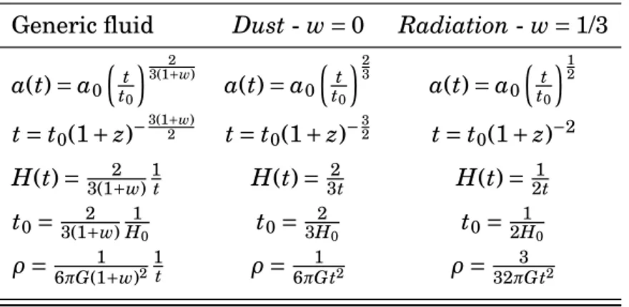
Table 2.1provides a list of some useful equations in the EdS Universe both for a generic fluid and for matter-dominated and radiation-dominated models.

TABLE 2.1 - Some useful relations in the EdS Universe: generic component

(left column), matter-dominated Universe (central column) and radiation-dominated Universe (right column).

Generic fluid Dust - w = 0 Radiation - w = 1/3 a(t) = a0 ³ t t0 ´ 2 3(1+w) a(t) = a0 ³ t t0 ´2₃ a(t) = a0 ³ t t0 ´1₂ t = t0(1 + z)−3(1+w)2 t = t0(1 + z)− 3 2 t = t0(1 + z)−2 H(t) =_3(1+w)2 1_t H(t) =_3t2 H(t) =_2t1 t₀₌ 2 3(1+w) 1 H0 t0= 2 3H0 t0= 1 2H0 ρ = 1 6πG(1+w)2 1 t ρ = 1 6πGt2 ρ = 3 32πGt2

Let us now briefly examine the curved cases, considering model with only a single component characterized by Ωw 6= 1. For small values of a or, equivalently, at high redshifts we have (2.64) Ω0 ³a₀ a ´1+3w À (1 −Ω0). If we introduce a critical value z∗(or a∗) so that

(2.65) Ω0

³a₀ a∗

´1+3w

=Ω0(1 + z∗)1+3w= |1 −Ω0|, when z À z∗(or a ¿ a∗), the relation (2.62) is reduced to (2.66) H(z) = H0Ω1/20 (1 + z)

3(1+w) 2 _.

Equation (2.66) is similar to what we found for an EdS Universe (eq. (2.63)), with the only difference thatΩ0 is not equal to one. Therefore it can be concluded that for high

redshift values, the curved models have the same behaviour of the EdS one. So, it is impossible to assess the curvature of the Universe, if we consider t too close to the Big Bang.

On the other hand, for z ¿ z∗(or a À a∗) for an open Universe (κ = −1) the expansion parameter grows indefinitely with time. While a closed Universe is characterized by the existence of an instant tm at which ˙a is zero and, after this time, the expansion parameter decreases. It implies that there is a second singularity (symmetrical in time with respect to the Big Bang) usually called Big Crunch.Figure 2.1below shows four possible scenarios (open, flat, closed andΛCDM models) for the evolution of the expansion parameter a as a function of time.

FIGURE 2.1 - Evolution of the expansion parameter a as a function of time for four possible scenarios. The orange curve represents a closed Universe (Ωm = 5 > 1), which initially expands, then turns around and collapses under its own weight (Big Crunch). The green curve describes a flat model (Ωm= 1) , in which the expansion rate continually slows down. The blue curve represents an open Universe (Ωm= 0.3 < 1) with a lower density than the previous two models. The red curve shows a Universe having a large amount of Dark Energy (Ω_Λ= 0.7), which causes an accelerated expansion of the Universe.

2.5. THEΛCDM UNIVERSE

2.5

T

HE

ΛCDM U

NIVERSE

By the beginning of the 21st century, the ΛCDM Cosmological Model, or simply the Standard Cosmological Model, was generally accepted. TheΛCDM predicts the presence of the Cosmic Microwave Background (CMB), which is the radiation left over from the recombination after Big Bang, but also describes very well the LSS of the Universe (such as clusters, galaxies).

According to this model, the Universe is composed principally by a radiative fluid with a negligible density, approximately 4% Baryonic Matter, about 26% Cold Dark Matter and for the remaining 70% an unknown form of Dark Energy (in the form ofΛ), the latter responsible of the accelerated expansion of the Universe (for more details on the estimates of these values, seePlanck Collaboration et al. 2016). The radiative fluid consists of relativistic particles and photons. This component does not play a fundamental role at z = 0, since its density parameter isΩ0,r≈ 10−5, as can be estimated from the CMB temperature measurement.

Regarding the matter component, the model assumes that the Universe is composed of both already mentioned baryonic and non-baryonic matter, also called ordinary matter and Dark Matter, respectively. The difference between the two matter components concerns their interactions. Though both of them are able to interact via gravity, just the ordinary matter can interact with photons. Fritz Zwicky in 1937 was the first scientist who proposed the existence of another kind of matter to explain the dynamics of galaxies in theComacluster (Zwicky,1937). By measuring the velocity dispersion of the galaxies inside the cluster, Zwicky estimated the average virial mass of the system be larger than 4.5 × 1010M_¯. However, the mass related to the luminosity of these “nebulae” was far smaller. Zwicky calculated a mass-to-light ratio of about 500, much larger than the ratio of about 3 measured for the local Kapteyn stellar system. Since the Zwicky’s discoveries and later works, from the 1970s many studies have been done in order to understand the nature of DM. For instance, Vera Rubin and Kent Ford measured the rotation curves ofM31, noticing a difference between the expected angular motion and the observed one (Rubin and Ford,1970). A large list of DM particle candidates have been suggested so far. It is thought that DM could be constituted by what are called weakly interacting massive particles (WIMPs), that is particles able to interact only through gravity and weak force (Jungman et al.,1996). Other studies investigated new theories of modified gravity to describe the observations without having to assume any form of non-baryonic matter (for a review, seeClifton et al. 2012).

Maddox et al. 1990,Efstathiou et al. 1990andGeller and Huchra 1989suggested that the CDM model was not able to explain the observed distribution of cosmological structures on very large scales. So they argued that the Universe is now lead by the Cosmological Constant.

Nowadays, theΛCDM model is broadly accepted, though most of its theoretical bases are still unexplained. In particular, the physical origin of the accelerated expansion is still unknown.

Insubsection 2.4.1we have derived the contribution of Cosmological Constant in the FLRW metric. If we set T_µν= 0, in equation (2.51) only theΛterm remains. It represents the energy of vacuum that provides a repulsive force in contrast to gravity.Λis described by an EoS with w_Λ= −1. It can be noted that density ofΛis constant throughout the expansion of the Universe (eq. (2.61)),ρ_Λ=Λc2/8πG (in line with the effective density term in eq. (2.53)).

The deceleration parameter is defined as follows:

(2.67) q(t) ≡ −a(t) ¨a(t)

˙ a2_(t) .

The deceleration parameter of a Universe composed of only matter, so with w = 0 and without any pressure term, is q =Ωm/2. This corresponds to a decelerated expansion (given the negative sign in eq. (2.67)), in contrast to observational evidences. Now let us consider a Universe composed of matter andΛ. The First Friedmann Equation will become (2.68) a = −aH¨ 2Ωm 2 + aH 2_Ω Λ= −aH2 µ Ωm 2 −ΩΛ ¶ = −aH2q.

If the expansion is accelerated, then q < 0 and the following condition has to be satisfied:

(2.69) Ω_Λ>Ωm

2 .

Moreover, q0 can be constrained from the relation between z and the magnitude of Supernovae type Ia. The current observations leads to a negative value of the deceleration parameter

(2.70) q0' −0.55,

corresponding toΩ0,m' 0.3 andΩ0,_Λ' 0.7. Adding together the individual valuesΩ0,wi,

the Universe results to be flat (P

iΩ0,wi = 1). As stated in the subsection 2.4.2, the

2.6. GRAVITATIONAL JEANS INSTABILITY

observed acceleration implies a change of ¨a at late times. This change (or flex) occurs at zf ' 0.68, as shown inFigure 2.1. By imposingΩm(zeq_Λ) =ΩΛ(zeq_Λ), we obtain the redshift equivalence, z ' 0.33. The observational fact that the present values of the densities of DE and DM are of the same order of magnitude implies that we are living in a peculiar moment of the history of the Universe. A density ratioρ_Λ,0/ρm,0≈ O (1) at the present epoch can be seen as coincidental, since it requires very special initial conditions in the early Universe. This is what is generally called the cosmological Coincidence Problem (Velten et al.,2014).

2.6

G

RAVITATIONAL

J

EANS

I

NSTABILITY

The Jeans theory on gravitational instabilities is now regarded as one of the cornerstones of the standard model. In 1902, Jeans demonstrated the existence of this instability in interstellar gas clouds to explain the formation of stars (Jeans,1902). Starting from a homogeneous and isotropic fluid, small fluctuations can evolve in time, when the internal gas pressure is unable to counteract the gravitational pull.

As discussed in section 2.5, the CMB, as a fossil of the density perturbations, presents fluctuations with small amplitude, observed close to the recombination epoch. By analysing the CMB spectrum, it has been possible to derive the amplitude of temperature perturbations

(2.71) δT

T ≈ 10 −5_,

where T = 2.72548±0.00057 K is the mean Black Body temperature of the CMB radiation (Fixsen, 2009). Current observations showed that the Universe seems to be rather inhomogeneous at megaparsec scales, as result of a non-linear evolution (Peacock and Dodds,1996).

The overdense regions of the Universe are capable to attract matter from nearby underdense regions. This process thus amplifies the inhomogeneities. The Jeans theory provides an analytical description of this phenomenon in the linear regime. It describes just non-relativistic matter, on scales inside the particle horizon, that is the spherical region causally connected with an observer defined as

(2.72) R_{H(t) ≡}

Z t 0

c dt0 a(t0₎.

The particle horizon separates two different regions. The region beyond RH is totally dominated by gravity, and needs a relativistic treatment. While on scales below RH, the Jeans theory can be used to describe the evolution of perturbations.

The Jeans instability describes the dynamics of a self-gravitating fluid. We shall begin by investigating the case of a collisional gas in a static background. Subsequently, we will extend the discussion to an expanding Universe towards a non-linear regime.

2.6.1 THEJEANS INSTABILITY IN ASTATIC UNIVERSE

By assuming the Newtonian approximation, we consider a homogeneous and isotropic fluid, having a constant matter density (ρ(x, t) = const) embedded in a static framework. The equations of motion of such a fluid are the following

(2.73)                                  ∂ρ ∂t + ∇ · ρv = 0 ∂v ∂t + (v · ∇) v + 1 ρ∇p + ∇Φ= 0 ∇2Φ− 4πGρ = 0 p = p(ρ, S) = p(ρ) dS dt = 0 .

These are the continuity equation, the Euler equation, the Poisson equation, the equation of state and the adiabatic condition, respectively. In this set of equations, v is the velocity vector of a fluid element,Φthe gravitational potential,ρ the density, p the pressure and S the Entropy. The last equation has been introduced, to neglect any dissipative terms, i.e. viscosity or thermal conduction.

Let us define the dimensionless density perturbation, the so-called density contrast, for the background as

(2.74) δ(x, t) ≡δρ(x, t)

ρ .

We consider small fluctuations, so thatδ ¿ 1. We can thus linearise the equations in (2.73). The density equation becomes a differential equation which in Fourier space reads

(2.75) δ¨k+ (k2c2_s− 4πGρ) δk= 0,

where k = |k| is the absolute value of the wavenumber, δk= δk(t) is the Fourier transform of δ(x, t), cs the speed of sound (as defined in eq. (2.56)). The previous differential equation has two independent solutions of the form

2.6. GRAVITATIONAL JEANS INSTABILITY where (2.77) ω(k) = q k2_c2 s− 4πGρ .

The solutions are of two types, according to whether the wavelengthλ = 2π/k is greater than or lower than the Jeans length:

(2.78) λJ= 2π k_J ≡ cs s π G_ρ.

In theλ < λJcase, we obtain two sound waves in the directions ±k, corresponding to two adiabatic perturbations with a phase velocity cph= ω/k. The latter tends to become equal to cs, when k À kJ (orλ ¿ λJ). Instead, whenλ > λJ, the frequencyω is imaginary and we obtain a non-propagating solution (stationary wave) of ether increasing or decreasing amplitude. The characteristic timescale for the propagation is

(2.79) _{τ = |ω|}−1= v u u u t 1 4πGρ0 µ 1 −³λJ λ ´2¶

For very large scales,λ À λJ, the gravity force leads and the perturbations can grow up with an exponential behaviour in time, tending to a free-fall collapse,τf f ∼ (G/ρ0)−1/2. This is the so-called Jeans instability.

2.6.2 THEJEANSINSTABILITY IN ANEXPANDING UNIVERSE

Let us now consider an expanding homogeneous and isotropic Universe. In this frame-work, the background density evolves as a function of time,ρB= ρB(t). The continuity equation becomes

(2.80) ρ˙B+ 3H(t) ρB= 0.

Now let us introduce a small perturbation into the set of equations (2.73) as before, and consider a double component velocity as

(2.81) _{u = ˙x = H(t)x + v}p.

The first term on the right-hand side of eq. (2.81) results directly from the Hubble Law, while the second term is the peculiar velocity due to the inhomogeneous distribution of matter in the Universe and it represents the perturbation with respect to the Hubble flow. Given that the unperturbed solutions have no scale dependencies, we can search for

solutions for each Fourier mode of the type shown in eq. (2.76). The resulting equation is the so-called dispersion relation

(2.82) δ¨k+ 2H(t) ˙δk+ (k2c2s− 4πGρ) δk= 0.

The 2H(t) ˙δk term is related to the Hubble friction, that hampers the growth of perturba-tions, while the k2c2_sδk term describes the characteristic fluid velocity. For wavelengths

λ such that the second term in the parenthesis of eq. (2.82) is lower than the first one and whenλ ¿ λJ with

(2.83) λJ' cs

s π Gρ,

we obtain two oscillating solutions. The solutions of this dispersion relation have the following form

(2.84) δ(x, t) = A(x)δ+(t) + B(x)δ−(t),

where A and B are two functions that depend on the comoving coordinates, while the time-dependent terms,δ₊andδ₋, represent the growing and decaying modes, respectively.

In theλ À λJ case there are two solutions, one of which leads to instability. Indeed, for an EdS Universe (withΩm= 1) the two solutions have the following trends:

(2.85) δ₋(t) ∝ t−1∝ a−3/2

and

(2.86) δ+(t) ∝ t2/3∝ a.

The first solution decays and does not give rise to the formation of structures, while the second one leads to gravitational instability.

For a Universe with a cosmological constant, the growing instability solution has the following integral form

(2.87) δ+(z) = H(z)

Z ∞ z

dz0(1 + z0) a₀H3_(z0₎.

A more complex model, describing a multi-component Universe, has not such a general integral expression, and so the differential equation has to be solved directly. We can provide an approximate formula to parametrise the previous findings, the so-called growth factor, as a function of the density parameter evaluated at z = 0:

(2.88) f (Ω0) =d logδ+ d log a 'Ω 0.55 m,0+ ΩΛ,0 70 µ 1 +1 2Ωm,0 ¶ .

2.6. GRAVITATIONAL JEANS INSTABILITY

This formula shows thatΛdoes not play a crucial role for the growth of the fluctuations. The exponentγ ' 0.55 is a result of General Relativity and it represents a method to test this theory on cosmological scales (Coles and Lucchin,2002).

2.6.3 THELINEAR REGIMETHEORY

To describe the distribution of matter in the whole Universe at a given cosmological time and its following evolution, one can divide the entire volume into several independent sub-volumes. Nevertheless, these sub-volumes will not stay independent long, because of gravity action. So, it is convenient to describe a generic fluctuation as a superposition of plane waves in Fourier space, that have the advantage to be independent during the evolution. This approach requires a statistical treatment of the initial perturbations.

The spatial Fourier transform of theδ(x) is

(2.89) δ(k) = 1

(2π)3 Z

δ(x)exp(−ik · x)dx. Let us define the Power Spectrum of the density field as follows

(2.90) 〈δ(k) δ∗(k0)〉 = (2π)3P(k)δ(3)_D (k − k0),

where δ∗_k = δ−k (because of the reality of δ) and δ(3)_D is the 3D Dirac delta function. Moreover, we introduce the two-point correlation function (from now on, 2PCF), that quantifies the spatial clustering of the objects, defined as

(2.91) ξ(r) = 〈δ(x)δ(x0)〉,

where r is the comoving distance between x and x0. It quantifies the probability excess, dP₁₂, compared with that expected one, of finding a pair of objects separated by a comoving distance r, in two comoving volume elements dV1and dV2, respectively:

(2.92) dP12= n2[1 + ξ(r)] dV1dV2,

where n is the mean comoving number density of the sample. The Wiener-Khintchine theorem relates the power spectrum to the two-point correlation function,ξ(r), (2PCF) via a Fourier transform:

(2.93) ξ(r) = 1

(2π)3 Z