Megistobenthic faunal diversity of the Antalya Gulf: Crustacea

(1)

ALMA MATER STUDIORUM – UNIVERSITÁ DI BOLOGNA

SCUOLA DI SCIENZE

Corso di Laurea Magistrale in BIOLOGIA MARINA

Megistobenthic faunal diversity of the Antalya Gulf:

Crustacea

Tesi di laurea in:

Biologia delle Risorse Alieutiche

Relatore Presentata da

Prof. FAUSTO TINTI ANNALISA PATANIA

Correlatore

Prof. ERHAN MUTLU

II sessione

(2)

1

1. Introduction

1.1 The importance of macrobenthos in the Mediterranean

Sea

The Mediterranean Sea is a semi-enclosed sea and occupies a huge depression, which reaches a depth of 5270 meters as its deepest point (depth average of 1480 m) and is a relatively small sea compared with other oceans. It is connected in its western part, to Atlantic ocean by the shallow strait of Gibraltar, and in the southeastern part is connected with Red Sea by the artificial Suez Canal, opened in 1869.

The general water circulation of Mediterranean sea is highly complex, from Strait of Gibraltar the less saline waters of the ocean enters through the surface waters, while dense saline waters flow beneath in deep in the opposite direction into the Atlantic Ocean (Millot, 1987). In the Mediterranean Sea the great rate of evaporation exceeds precipitation and river runoff (Malonette-Rizzolli et al, 1999) causing a high salinity of the waters, from about 38 to 39.5 psu by the stratification of the water column. Furthermore, there are many hydrological characteristics of the Mediterranean Sea, such as the high oxygen concentrations and a decreasing of nutrient concentrations from west to east, which affect the structure of the pelagic food web, causing strong oligotrophic conditions (Danovaro et al., 1999).

For its environmental structure, the Mediterranean marine ecosystem is highly vulnerable to perturbations, and it is going to rapid changes mainly due to the intense anthropogenic activity, that involve climatic changes, pollution, an over-exploitation of marine living resources with fishery, the establishment of alien species.

The impact of these pressures is leading to a degradation of Mediterranean ecosystem, so for this reason is necessary to have tools to study and monitoring the functioning of marine ecosystem to improve the identification of the main operative task to restore compromised equilibrium. The study how the biotic component responds to changes in the physical environment is an essential step to predict the consequences of these changes on the

marine ecosystem. For this purpose, benthic organisms are superior to many other biological groups for their response to environmental stresses, providing fundamental data that are relevant to general objectives of most marine monitoring programs (El Komi and Emara, 2007).

(5)

4 Benthos or benthic organisms are referred as to all organisms that are living in or closely associated with the sea bottom (Stirn, 1981). The combination between river discharges and marine currents carries large amounts of suspended sediments to bottom regions, impacting the local ecosystems. Benthic communities play an important role in the marine ecosystems, being food for fish and cycling nutrients between the sediment and the water column. The amount of production and the part that is passed on the demersal fish via benthic organisms can be estimated qualitatively and quantitatively (Arntz, 1978).

The benthos is divided according to size in three classes:

 Macrobenthos: mainly organisms that are retained by sieves of 0.5 mm. This class can be further subdivided into megistobenthos (>25 mm), megabenthos (2-25 mm) and mixobenthos (0.5-2mm) (Bacescu et al,1971).

 Meiobenthos: organisms with size between 0.5 mm and 63 μm

 Microbenthos: organisms with size less than 63 μm

Benthic macrofaunal assemblages are important in the marine ecosystems that display a great variation in species composition of polychaetes, molluscs, echinoderms, and

crustaceans living in burrows in the sediment (infauna) or on the sediment surface (epifauna). These assemblages represent the basic level of trophic chains, being food source for many species of commercial fish and shellfish.The variability of benthic assemblages on a site can reflect, in an integrative mode, the entire functioning of the marine ecosystem, representing a sum up of effects, which environmental factors have on each individual during a longer period and minimizing the adverse impact particularly on the marine ecosystem (El Komi and

Emara, 2007). Macrobenthic communities have long been considered as a possible

indicators for monitoring any anthropogenic impact or natural long term alterations in marine ecosystems, providing valuable information that cannot otherwise be obtained from other biological groups, because they adapt responding to environmental stresses (Bilyard, 1987; Kroncke, 2003).

A huge variety of environmental sourcesaffect the biodiversity pattern of benthic organisms, in different ways. Substrate types, such as hard and soft bottoms and vegetative marine beds, play an important role on species richness and diversity pattern of benthos (Beaman and Harris, 2007; Kostylev et al, 2001). Other factors can structure the spatial benthic assemblages, such as the levels of dissolved nutrients (Cinar et al, 2012), the oxygen

(6)

5 content in the near bottom waters (Seitz et al, 2009) and total organic carbon content of the sediment and bottom depth (Mutlu and Ergev, 2013).

Macrofauna includes many phyla of invertebrates, but is generally considered that the most important taxa are molluscs, crustaceans and polychaetes (McLachlan, 1983). Benthic crustaceans are an important source of foods consumed by human, and have a relevant importance in nutrition of other marine organisms. Theyhave been considered to be the most sensitive communities to changes in environmental variables, so they are good biological indicators for monitoring the ecological status of marine ecosystem and water quality (Gesteira & Dauvin, 2000; Kramer et al. 2013; Sanchez-Moyano & Garcia-Gomez, 1998).

1.2 The Levantine Sea: environmental and ecological features

The study area is located in the Antalya Gulf, Levantine sea (Figure 1). The Levantine basin is the second large and easternmost basin of the Mediterranean Sea. It is surrounded by the coast of Libya, Egypt, Israel, Lebanon, Syria, Turkey, and Cyprus, and thewhole area is constantly subjected to anthropogenic inputs, particularly in the fishing grounds. The

ecosystem of Levantine Sea has been affected by significant changes of fauna and flora due to biological invasion of Lessepsian species (i.e. marine species of Indo-Pacific origin

(7)

6 Figure 1 Location of study area

The continental shelf of the Levantine basin is generally very narrow with the exception in Mersin and İskenderun Bays, and in the region of Antalya there is one of the major troughs (with water depth of 1500 meters) of the northern Levantine basin (Ozsoy et al., 1993). The different features of hydrography and climatology in the Levantine basin allow four distinct water masses in the water column profiles: i) the Levantine Surface Water, that is warmest (16-25 ⁰C) and saltiest (38.8-39.4 psu); ii) the second is the Modified Atlantic Water, which originates from the Atlantic Ocean and it can be identified from salinity minimum (38.5-39 psu and about 17 ⁰C); iii) the Levantine Intermediate Water (LIW), the saltiest water mass of eastern Mediterranean thatoccupies the intermediate layers between 200 and 700 meters depth (39.1 psu and 15.5⁰C); iv) the Levantine Deep Water, which is the colder and less saline than the LIW, with 38.7 psu and 13.6 ⁰C (Ozsoy et al., 1989 and 1993). The LIW is formed by the cooling of the surface saline waters during winter, which are transported westward at a depth between 300 m and 500 m towards the Strait of Sicily and then towards Gibraltar. The eastern Mediterranean deep waters drops into the deeper parts of the basins, and these sinking waters carry all the nutrients through the deeper layers. This is one of the reasons why Levantine Sea is one of the world’s poorest basins in terms of nutrient sources (Ozsoy et al., 1993).

(8)

7 In any case, as underlined before, is well known that all the Mediterranean Sea is poor in nutrient, and that the nutrient amount decreases from western to eastern part of the

Mediterranean. This is mainly due to a limited external input and to a more intensive leakage of polluted river waters into the western part. Therefore these waters are ultra-oligotrophic and fluctuations of nutrient concentration were observedthroughout the year. It has to be noted that during spring these waters displayed a low nutrient loadin the surface (Uysal and Koksalan, 2006). In addition, the eastern Mediterranean has low plankton biomass and production (Stergiou et al., 1997). The Eastern Mediterranean has some of the world’s most optically clear waters and the Secchi disc transparency ranges from 20 to 38 m depth (Ediger and Yılmaz, 1996).

These environmental conditions of Levantine waters (i.e. the scarcity of nutrient concentration, the continuous entering of invasive species, and the particular physical conditions) can lead to additional pressure on natural resources, and these could be considered the factors that mainly affect the benthic community structure.

Most of the previous benthic studies conducted were concentrated in the western part of Mediterranean Sea (Tselepides et al., 2000). Furthermore,the number of species in the Mediterranean has been changed with the increasing number of the Lessepsian invaders especially in the Levantine area. In the last two decades, many studies carried out in the Levantine area have been focused on the native and non-native species diversity of the benthic crustaceans, with new records ofalien species and of crustaceans hugely reported in the Turkish waters (Cinar et al, 2006; Yokes and Galil 2006 ; Ozcan et al, 2006; Dogan et al, 2008). Until now, the number of marine alien arthropods in Levantine coast of Turkey is of 65 species, with a hot spot in the Iskenderun Bay, due its proximity to the Suez Canal (Bakir et al, 2014).

Nevertheless, also many studies were interested on distribution and ecological status of macrobenthic organisms in Turkish Levantine waters. For instance, Bingel et al. (1995) reported a total of 141 benthic species in Manavgat (the same area of the present study) with dominant taxa Annelida (67) and Mollusca. Gücü et al. (2001) identified 84 species in the İskenderun Bay with Annelida and Mollusca as dominant groups. An exhaustive study on benthic communities (infaunal and epifaunal communities) in the Mersin bay was conducted by Ergev (2002), in which 122 epibenthic species were reported with Annelida as the

(9)

8 communities in Cilician Shelf (northeastern part of Levantine) and identified 692 species of macrobenthos and the Annelida as dominant group. According to results of various studies on the benthos in the eastern part of Mediterranean Sea (Çınar et al., 1998; Tselepides et al., 2000; Gücü et al., 2001; Ergev, 2002; Uysal et al., 2008; Mutlu and Ergev, 2007) Annelida was the main dominant group in the benthic communities and it was generally followed by Mollusca or Crustacea.

Since each dominant taxa of benthos showed different response to a variety of environmental parameters, some studies have recently concerned the spatio-temporal distribution of benthic assemblages and their relationships with environmental factors were assessed in many areas of Levantine basin (Mutlu and Ergev, 2012; Mutlu and Ergev, 2013; Mutlu, 2015). In the Gulf of Antalya, some ecological distribution studies were done (Ergen and Cinar, 1997; Cormaci and Furnari, 2002) but there have been no significant studies until now on spatial and temporal distribution of benthic crustaceans that related their community to ecological factors in this area.

Many alien benthic crustaceans are well established in the Levantine Sea replacing or filling the gap of ecological niches responded by the native benthic crustacean species (Mutlu, 2015). Moreover these invaders speciesplay a conspicuous role in the host ecosystems, threatening native species, and they could affect the crustacean trawl fishery of the Levantine Sea with negative economic consequences (Boudouresque and Verlaque, 2005 ).

Crustaceans, such as lobsters, crabs, and penaeid shrimps are very important for fishery due to high demand in the markets. In Europe, approximately 22 crustacean species are fished commercially. The crustacean trawl fishery inthe Levantine area is very common and has an important role due to its quantity and the economic value of its landings. For its economic value, the crustacean fishery, particularly of penaeid shrimps, has been carried out using a specially designed bottom trawl that is called “shrimp trawl” in the easternmost part of Levantine Sea (Can et al., 2004).

However, all the Levantine coasts of Turkey are strongly subjected to crustacean fishery with the traditional trawl net, especially to catch high-value decapods. Ten shrimp species have been reported to be commercially important for Turkish trawl fisheries in the Levantine Sea: Penaeus semisulcatus, Melicertus kerathurus, Marsupenaeus japonicus, Parapenaeus longirostris, Metapenaeus monoceros, M. stebbingi, Trachypenaeus curvirostris, Melicertus hathor, Aristaeomorpha foliacea, Plesionika heterocarpus (Bayhan et al., 2003).

(10)

9

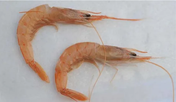
1.3 Parapenaeus longirostris

The common name of Parapenaeus longirostris (Lucas,1846) is deep-water rose shrimp, for its distribution and its coloration. This shrimp shows a wide bathymetric distribution, occurring from 20 to 750 m depth and being more abundant in bathyal zone between 100 and 400 m depth on sandy and sandy-mud bottoms (Sobrino, 1998; Tom et al., 1988). However, biomass is higher between 200 and 400 m depth, showing a marked, size-dependent

distribution with depth, with small individuals being found at the edge of the continental shelf (Abelló et al., 2002). This demersal species has a wide distribution, being present in the entire Mediterranean as well in the eastern Atlantic from Portugal to Namibia (Pérez-Farfante & Kensley, 1997). The species plays an important ecological role in many demersal

communities of the continental shelf and upper part of the continental slope (Sobrino et al, 2005) .

Like all penaeids, the body of the deep-water rose shrimp is laterally compressed and the part of cephalothorax is protected from a carapace.Its color is pink - orange, darker in the carapace and in the rostrum. In females the coloration of gonads fluctuates from white to greenish, depending on the sexual maturity stage. there is a distinctive The epigastric tooth of the cephalothorax and the straight or slightly curved carapace rostrum with 7 dorsal teeth and without teeth in the ventral part are distinctive features distinguishing the deep water rose shrimp from other penaeids (Falciai and Minervini, 1992). The surface of the shrimp cuticle is smooth and free of bristles. On the lateral part of carapace a longitudinal sutures extending from postorbital margin to almost posterior margin. An antennal spine, an hepatic spine and an branchiostegal spine are present in the lateral part of carapace. The telson is armed with three teeth fixed. Petasma is symmetrical and semiclosed and thelycum is closed (Sobrino et al, 2005).

The deep water rose shrimp is one of the most important commercial decapoda species in bottom trawl fisheries throughout its distribution range, in Atlantic and Mediterranean waters, where it is caught as target or by-catch (Ribeiro-Cascalho and Arrobas, 1987). Regarding the crustaceans with commercial value in the Mediterranean Sea, this shrimp is the fifth in order of importance considering the total biomass landed (Stamatopoulos, 1993). In Turkish waters, total reported catches of Parapenaeus longirostris were 2501.8 tons in 2014 and 93.9 tonsof these were from the Levantine Sea (TUIK, 2015).

(11)

10 Because of its great commercial importance, many studies were carried out in the last

decades regarding Parapenaeus longirostris, which have permitted to have an assortment of detailed information on its biology, distribution, abundance, fishery and stock assessment (Abelló et al., 2002; Bayhan et al., 2005; D’Onghia et al., 1998; Guijarro et al, 2009; Sobrino, 1988 , etc).

(12)

11

1.4 Objectives

This thesis deals with to analyze the spatial and temporal distribution of the megistobenthic crustacean assemblages of Antalya Gulf. In order to provide a comprehensive overview of the spatio - temporal patterns of crustacean community, I have also investigated the correlation of biological data of assemblages with a set of environmental parameters, including physical, chemical and bottom features of the study area.

Furthermore, for its economic importance in Levantine waters, a focus analysis was done to obtain information of morphometric characteristic and study the length frequency composition of the Parapenaeus longirostris population of the Antalya Gulf where it is an important target species of fishery.

(13)

12

2. Materials and Methods

2.1 Study area and sampling

The study was conducted on the Turkish continental shelf off the Antalya Gulf,within infra-littoral and circa-infra-littoral zones. The Gulf of Antalya is subjected to high intensity human uses linked to coastal zone pressures such as tourism and maritime traffic, especially during summer. In the study area there are the Manavgat river and two little streams, which represent the major sources of freshwater in the Antalya Gulf. Throughout the year, in the area of Antalya, fishing is not allowed within 2 miles of the coast. The sampling stations were located in two different areas. The first area is open to fishing and covers the region of the towns of Lara and Side. The second area is a closed fishing area and includes the region between the cities of Side and Gazipasa. In this area any kind of trawling is forbidden according to the Turkish law (RG 26.02.2005 / 25739).

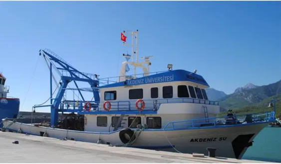
The data analyzed in the present work derived from experimental trawl surveys within a framework of the project no: 2014.01.0111.001 supported by Scientific Research Project Coordination Unit of Akdeniz University. Samples were collected by the R/V “Akdeniz Su” (fig 3) (total length 26.5m, 670 kW of engine power) of the Faculty of Fisheries, Akdeniz

University.The data were collected in May, August and October 2014, and February 2015, thus representing the seasons of the year.

(14)

13 .

Samples were collected on three oceanographic transects. called T1, T2 and T3. T1 and T2 were situated in the area open to fishery, while T3 in the no-fishing area. Each transect consisted of five different depths: 10, 25, 75, 125, and 200 m depth. Furthermore, during each cruise additional hauls were carried out at 300 m depth in T1 and T3, and for each cruise intermediate stations between the transects in order to provide a better ecological and environmental characterization of the area. In figure 4 and table 1 are shown the sampling sites in the study area, and the coordinates of sampling stations with corresponding code (i.e. for T1 station at 10 m depth of August cruise the code is AT1_10) .

The duration of each haul (bottom time) was about 30 minutes and position was recorded with Global Positioning System (latitude and longitude) in 5 second intervals from the start to the end of trawling.

The sampling device was a polyethylene otter trawl net with a float line length of 15.3 m. The cod end had a square mesh opening of 44 mm, as usual commercial net. This cod end was protected by a polyamide cover net with 25 mm mesh size.

(15)

14 Figure 4 Sampling stations in each season in the Antalya Gulf.

(16)

15 Table 1 Coordinates of sampling stations for each season in Antalya Gulf

Sta ti on La ti tu de (⁰ N ) Lo ng itu de (⁰ E) Sta ti on La ti tu de (⁰ N ) Lo ng itu de (⁰ E) Sta ti on La ti tu de (⁰ N ) Lo ng itu de (⁰ E) Sta ti on La ti tu de (⁰ N ) Lo ng itu de (⁰ E) T1 _1 0 36 .8 41 32 34 6 30 .8 78 10 00 3 T1 _1 0 36 .8 41 34 12 8 30 .8 90 80 23 3 T1 _1 0 36 .8 41 26 33 8 30 .8 83 09 69 6 T1 _1 0 36 .8 42 18 38 7 30 .8 89 02 55 5 T1 _2 5 36 .8 27 74 39 5 30 .8 92 63 57 8 T1 _2 5 36 .8 27 72 92 3 30 .8 93 66 98 8 T1 _2 5 36 .8 28 65 71 8 30 .9 48 65 81 9 T1 _2 5 36 .8 27 42 75 6 30 .9 01 98 69 9 T1 _7 5 36 .8 03 19 50 3 30 .9 05 83 65 9 T1 _7 5 36 .8 05 76 88 6 30 .8 96 54 41 8 T1 _7 5 36 .8 03 53 8 30 .9 35 63 65 T1 _7 5 36 .8 07 69 85 8 30 .8 85 65 77 T1 _1 25 36 .7 85 48 03 2 30 .8 84 96 54 7 T1 _1 25 36 .7 85 17 35 9 30 .8 72 14 24 3 T1 _1 25 36 .7 84 05 98 30 .8 87 29 76 7 T1 _1 25 36 .7 87 67 65 9 30 .8 74 91 18 T1 _2 00 36 .7 67 59 55 2 30 .9 07 11 53 4 T1 _2 00 36 .7 68 15 58 30 .8 96 36 23 9 T1 _2 00 36 .7 69 25 34 2 30 .9 06 50 00 8 T1 _2 00 36 .7 66 33 42 7 30 .8 97 05 84 7 T1 _3 00 36 .7 46 34 71 4 31 .1 16 16 18 T1 _3 00 36 .7 45 25 83 6 31 .1 09 42 59 5 T1 _3 00 36 .7 43 43 59 7 31 .1 14 63 75 6 T1 _3 00 36 .7 44 76 54 8 31 .1 10 40 77 5 T2 _1 0 36 .8 00 24 17 2 31 .3 15 65 84 9 T2 _1 0 36 .7 96 48 05 1 31 .3 17 01 51 4 T2 _1 0 36 .8 01 18 47 6 31 .3 11 75 95 6 T2 _1 0 36 .8 03 21 12 31 .3 08 87 11 1 T2 _2 5 36 .7 76 94 62 4 31 .3 00 23 91 9 T2 _2 5 36 .7 79 59 73 3 31 .2 93 38 60 7 T2 _2 5 36 .7 76 74 45 3 31 .2 94 20 88 T2 _2 5 36 .7 79 15 63 9 31 .2 96 66 38 7 T2 _7 5 36 .7 52 19 68 4 31 .3 15 71 84 4 T2 _7 5 36 .7 54 06 49 31 .3 08 38 28 8 T2 _7 5 36 .7 60 34 17 3 31 .2 81 50 35 7 T2 _7 5 36 .7 54 07 92 5 31 .2 97 29 60 3 T2 _1 25 36 .7 49 85 68 1 31 .2 87 32 16 8 T2 _1 25 36 .7 53 39 86 3 31 .2 76 43 66 7 T2 _1 25 36 .7 48 96 92 31 .2 91 90 71 2 T2 _1 25 36 .7 49 09 90 2 31 .2 86 38 76 4 T2 _2 00 36 .7 40 69 15 5 31 .3 18 47 69 T2 _2 00 36 .7 36 40 67 7 31 .3 13 84 55 2 T2 _2 00 36 .7 39 17 12 1 31 .2 99 99 64 3 T2 _2 00 36 .7 42 41 69 3 31 .2 84 16 43 T3 _1 0 36 .7 17 20 09 6 31 .5 29 22 60 1 T3 _1 0 36 .7 22 93 57 7 31 .5 15 89 39 1 T3 _1 0 36 .7 21 39 81 9 31 .5 19 68 16 T3 _1 0 36 .7 37 04 43 4 31 .4 75 99 96 3 T3 _2 5 36 .7 33 30 74 7 31 .4 55 68 79 7 T3 _2 5 36 .7 32 72 50 3 31 .4 61 41 62 4 T3 _2 5 36 .7 32 11 20 2 31 .4 66 99 74 T3 _2 5 36 .7 34 00 21 6 31 .4 53 20 56 6 T3 _7 5 36 .6 83 92 85 31 .5 60 45 33 3 T3 _7 5 36 .6 92 29 98 2 31 .5 48 90 62 3 T3 _7 5 36 .6 86 34 90 2 31 .5 55 85 65 1 T3 _7 5 36 .6 73 01 97 7 31 .5 83 89 58 3 T3 _1 25 36 .6 76 71 46 8 31 .5 65 39 15 T3 _1 25 36 .6 71 22 20 8 31 .5 74 67 21 6 T3 _1 25 36 .6 74 84 51 5 31 .5 67 78 73 5 T3 _1 25 36 .6 76 82 57 5 31 .5 66 14 24 2 T3 _2 00 36 .6 62 72 58 4 31 .5 68 92 01 6 T3 _2 00 36 .6 67 67 45 4 31 .5 65 74 69 3 T3 _2 00 36 .6 77 71 06 6 31 .5 48 14 64 9 T3 _2 00 36 .6 77 11 55 3 31 .5 46 32 71 7 T3 _3 00 36 .6 93 09 61 5 31 .4 40 63 79 7 T3 _3 00 36 .6 93 88 77 8 31 .4 24 44 20 4 T3 _3 00 36 .6 97 70 13 31 .4 16 45 54 9 T3 _3 00 36 .6 96 67 90 4 31 .4 27 37 32 1 T4 _6 5 36 .7 57 29 24 9 31 .3 39 46 72 7 T3 _5 0 36 .6 98 29 05 31 .5 37 88 46 9 I_ 10 36 .8 17 32 15 4 31 .1 74 99 52 3 I2 _3 0-60 36 .7 82 11 78 1 31 .2 26 59 89 7 A _5 0 36 .8 16 89 15 8 30 .9 10 54 85 6 I_ 40 36 .7 90 79 02 4 31 .1 60 35 57 4 I3 _1 5 36 .8 19 97 18 2 31 .1 23 87 17 3 A _1 00 36 .8 05 70 95 3 30 .9 73 19 17 8 I4 36 .7 88 26 28 8 31 .0 12 17 33 A 2_ 15 36 .8 14 04 10 7 31 .1 42 49 88 2 I5 _1 00 36 .7 82 78 61 1 30 .8 98 80 00 1 9 - 1 5 Fe br ua ry 2 01 5 11 - 16 M ay 2 01 4 Ta bl e 1: C oo rd in at es of sa m pl in g st at io ns fo r e ac h se aso n 20 - 27 A ug ust 2 01 4 20 - 27 O ct ob er 2 01 4

(17)

16

2.2 Onboard work

2.2.1 Collection of benthic communities

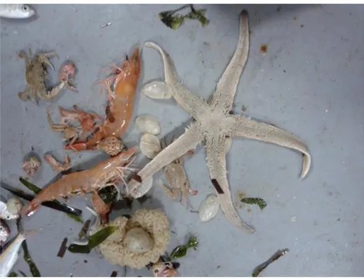
The organisms were caught with cod-end and cover net, and the operations described below were carried out for both types of device. For each haul, a preliminary sorting was carried out to separate megafauna (crustaceans, sponges, and molluscs) from fishes and no-living inorganic and organic materials such as litters (Fig. 5). Afterward, the sorted megafaunal organisms were stored in plastic jars and were fixed with 5% formalin-seawater solution buffered with borax (40 g for each liter of formalin-seawater) for laboratory analysis. Very abundant species were subsampled randomly by weight to provide a representative sample of the species.

(18)

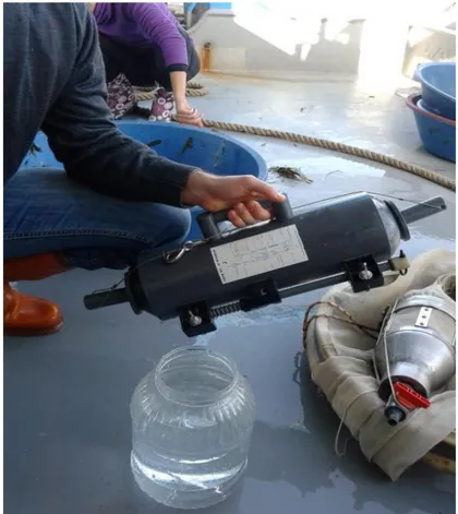
17 2.2.2 Environmental parameters

The environmental parameters considered in this study were chemical, physical, biological and sedimentary parameters (measured at surface and near bottom water, see table 2). All the parameters have been generally collected just before the sampling or at the end of the trawl operations picking up a sample of seawater using a polyethylene Nansen bottle (fig. 6). The transparency of water was measured by a Secchi disk, a 30 cm-diameter plain black-white circular disk that is lowered by hand into the water column until to the depth at which it is no longer visible. The length at which the disk vanishes is called the Secchi depth, and is taken as measure of transparency.

The salinity, dissolved oxygen, temperature, pH and conductivity were measured with a YSI multi-parametric probe. The density of the seawater (ρ) was calculated using the equation from Fofonoff & Millard (1983). The same seawater sample was used to analyze the total suspended material and chlorophyll-α. To determine the suspended material, one liter of seawater was filtered onto a microfiber filter with a retention of 1.2 μm using a vacuum pump with a filtered funnel and a graduated cylinder.

Table 2 List of environmental parameters as physical, chemical, biological and sedimentary (Superficial sediment) parameters measured at the sampling stations and abbreviations of the parameters used in the analyses.

Physical and chemical parameters Biological parameters Sedimentary

parameters classified with VBT

Secchi disk depth (m) Seston - 1 mm (g); Se1

Temperature (⁰C); SST and NBT Seston - 0,5 mm (g); S2 1; Rocks covered with Posidonia Salinity (PSU); SSS and NBS Seston - 0,063 mm (g);

S3

2; Muddy sand Oxygen (mg/L); SSOx and NBOx Bioseston - 1 mm (g); Bi1 3; Sand

pH; SSpH and NBpH Bioseston - 0,5 mm (g); Bi2

4; Mud Density, sigma-t; SSD and NBD Bioseston - 0,063 mm

(g); Bi3

5;Sandy mud Conductivity (S/m); SSC, and NBC Tripton - 1mm (g); Tr1

Chl-α (mg/mL); SSChl and NBChl Tripton - 0,5mm (g); Tr2 Total suspended matter (mg/mL);

STSM and NBTSM

Tripton - 0,063mm (g); Tr3

(19)

18 For the chlorophyll analysis, one literof seawater was filtered onto a filters of 0.7 mm pore size and 47 mm of diameter using a vacuum of less than 0.5 atm. The filters were stored in the freezer (< 0°C) until the laboratory analysis.

Furthermore, seawater samples were collected by a Nansen Closing net to analyze the zooplankton of each haul. At the end of the haul, the outer side of the net was scattered down with surface seawater to concentrate the organisms in the collecting container. The samples were size-fractionated through a series of sieves of 1, 0.5 and 0.063 mm mesh size, and each size was filtered onto a glass fiber filters through vacuum pump. Lastly the samples were frozen for treating in the laboratory.

(20)

19

2.3 Laboratory work

2.3.1 Environmental parameters

Each filter of total suspended material, after defrosting at room temperature, was dried in an oven at 60°C for 24h. The dry weight of filters was measured on an analytical balance

(Radawak A220) . The final amount of suspended material was obtained by subtracting to the dry weight of suspended material the weight of the empty filter after drying.

The Chlorophyll-α amount (Chlα, mg/mL) was assessed with an acetone-extraction method. Filters were homogenized with 10mL of acetone solution (90%) and maintained in the dark and cold. After 24h, samples were gently centrifuged and absorbance was measured at different wavelength (665, 645 and 630 nm) at the spectrophotometer. The filtered samples were blanched with a solution of 90% of acetone at 750 nm wavelength. The [Chlα] was calculated with the following equation:

[ ] where

Va is the acetone volume (expressed in mL) and l path length of cuvette (cm) and V is filtered seawater sample volume (mL) (Lorenzen, 1967).

The zooplankton analysis was carried out as following: after defrosting at room temperature, each filter was dried in an oven at temperature of 60⁰C for 24h and weighted on an analytical balance to determine the dry weight. Then each filter was reduce to ashes in a muffle furnace at 500⁰C for 6 hours, and weighted again. Furthermore, three aliquots of filtered seawaters were treated in the same way described above to determine the blanks. The mean dry weight of blanks was subtracted from the measured dry weight of sample seawater to determine the total organic and non-living matter (Seston). The ash weight, which represents the inorganic fraction (Tripton), was subtracted from the dry weight for determination of the organic fraction (Bioseston).

The information on bottom types is encoded in the echo-signal of the echo-sounder and acquired simultaneously with GPS data. During surveys different echoes can be observed on the oscilloscope: hard bottoms produced a sharp echo-signal type of high amplitude while soft bottoms produced an elongated echo-signal type of low amplitude. In order to classify

(21)

20 the different bottom types the Fractal Dimension method implemented in Bio Sonics Bottom Classifier VBT was used in this study. In this software, the Fractal Dimension (FD) is a measure of the irregularity of an echo envelope obtained from the bottom. By classifying the echo-signal envelope in terms of its FD, the shape of the envelope can be defined by

associating it with a FD number. Since the echo envelopes associated with different bottom types show regularities in shape, bottom echoes can be classified as function of FD.

2.3.2 Sorting and identification

The benthic crustaceans were sorted out from megafauna jars and transferred in a 70% ethanol-water solution, keeping cod-end and cover organisms separated. After sorting, crustacean specimens were identified and recognized to species level or to the lowest possible taxonomic level. Olympos binocular Stereomicroscope was used to examine the details of appendages of tiny species. Keystone and common species for each station were identified.

Taxonomic identification of species were based principally on “Mediterranee et mer Noire Volume I” (Fischer, 1973) and the checklist WoRMS (World Register of Marine Species, http://www.marinespecies.org ). For a better identification of Lessepsian species it was consulted the website of CIESM (Atlas of Exotic Species in the Mediterranean).

2.3.3 Biomass and Abundance

After identification, the abundance and the wet-weight (biomass) of each species were calculated. To determine the weight, all specimens were put on a paper for a while and then weighted by using a digital balance to the nearest precision of 0.001 g.

To study the length-weight relationship of commercial species, individual size was measured with a digital caliper to the nearest precision of mm.

Different biometrical measurements were taken for each taxonomical group, in relation to the morphology of species. The analyzed species were Marsupenaeus japonicus, Penaeus hathor, Penaeus semisulcatus, Melicertus kerathurus and Parapenaeus longirostris, Maja squinado, and Squilla mantis. Here in the thesis, how just said, I focused only on deep-water rose shrimp Parapenaeus longirostris.

(22)

21 For each specimen of Parapenaeus longirostris the following biometrical measurements were taken:

 Carapace length (CL) from the inside of the eye socket to the posterior margin of cephalothorax (Holden and Raitt, 1974).

 Carapace width (CW) the maximum width of cephalothorax

 Total length (TL) from the tip of the eye socket to margin of the telson.

The sex was determined observing the presence of petasma in males, or the thelycum in females. Individual whose sex determination wasn’t possible because decomposed or deformed were classified as not identified.

2.4 Statistical analysis

2.4.1 Environmental parameters

All environmental data of four seasonal cruises were organized in a matrix (in the first column the list of environmental parameters and in the first row the stations), and were normalized to allow comparison between different unit of measurement.

Based on these normalized physical variables, Principal Components Analysis (PCA) was applied to create an ordination that highlight the explanatory environmental variables and components of spatio-temporal description of the study area. The technique consists in ordering the point-sample along the axes (one for each variables). The goodness of representation of the point-sample is evaluated by the variance of the first two axes. This analysis was based on dissimilarity matrix created on Euclidean distance coefficient and was performed by PRIMER-E v6 (Clarke and Gorley,2006).

The formula of Euclidean distance index is:

√∑( )2

Where j,k are the countable indices of samples, and i=1…p are variables used in the analysis.

(23)

22 The software SURFER was used to plot the graphs of explanatory environmental parameters (density, temperature, dissolved oxygen and salinity) for each season to show main differences among depths.

2.4.2 Crustacean community analysis

Thebiomass (g) and abundance (N) data collected in the laboratory for each species, were organized into two arrays. Each matrix showed in the first column the list of species and in the first row the stations. In the same files was added the value of subsample measured onboard for each haul. For each station abundance (N/Km²) and biomass (g/Km²) data were standardized using the trawling area. The trawling area was calculated over the coordinates obtained by the GPS and using the head rope length (35 m) (Sparre, 1998). Sampling dates and coordinates of stations are shown in Table 1. At the end, biomass and abundance data of cod-end and cover net were sum up together for each station, and over these data all the analysis were performed.

At first a qualitative and quantitative description of the crustacean community of area was done (over biomass and abundance) based on the following three numerical indices:

1) Frequency of occurrence is expressed as the percentage of total frequency of occurrence of all species in the study area (Holden and Raitt, 1974).

2) Numerical occurrence is defined as the total individual percentage of each species among total individuals of all species in study area (Holden and Raitt, 1974).

3) Dominance (Soyer index) is similar to frequency of occurrence method, this is a qualitative distribution of occurrence percentage of each species among the stations. According to Soyer (1970), species with D>50% are considered constant species, those with D between 25% and 50% are common species while those with D values > 25% are considered rare.

For the preliminary analysis of the crustacean community the abundance and biomass data were estimated per square meter.

As an indication of crustacean faunal characters, a set of diversity indices was calculated. The number of species (S) the abundance of species (N), the biomass of species (B), Margalef’s index (d), Pielou’s evenness (J’) and Shannon-Wiener diversity (H’, log e base) indices were calculated for each seasons, transect and depth. These indices were calculated

(24)

23 with diverse function of PRIMER-E v6 The main aim of these faunal indices is to reduce the multivariate information of assemblage data in a single index, which can be easily handle by univariate analysis (Clarke and Warwick, 2001).

The formulas of these indices are the following:

 Abundance of individuals (N) is the number of individuals present in the sample

 Species richness (S) is given as the total number of species present in the sample.

 Margalef’s index (d) is an index of species richness, which also incorporates the total number of individuals (N) and is a measure of the number of species present for a given number of individuals:

 Shannon-Wiener diversity (H’, log e base) is the most commonly used diversity measure:

∑

Where pi is the proportion of the total count arising from the ith species.

 Pielou’s evenness (J’) is an expression of equitability in the sample, that is how evenly the individuals are distributed among the different species, and is expressed as:

Where H’max is the maximum possible value of Shannon diversity (Clarke and Warwick,

2001).

Three-way ANOVA was tested for each diversity indices among seasons, transects and depths. This univariate analysis was done with software IBM SPSS Statistics 21.

Spatio-temporal changes in crustacean community composition were visualized from multivariate analysis based on triangular matrices of Bray-Curtis similarities using transformed data. The biomass and abundance data were transformed with method “Taylor’s power law” with log(x+1) to weight the influence of common and rare species. The Bray-Curtis similarity index was used to create a similarity matrix between samples (stations) for both abundance and biomass transformed data.

(25)

24 This index was chosen because provides more reliable results in the study of benthic communities (Faith et al, 1987) . The formula of Bray-Curtis index is the following:

(

∑ | |

)

Where Sjk is the similarity distance between samples j and k, and xij is the value of individuals

of species i in sample j and xik is the values of species i in sample k.

Based on similarity measures of the Bray-Curtis index, the Hierarchical Cluster Analysis was done, and results were displayed in a dendrogram. This is an agglomerative method employing group-average linking, used to examine assemblages grouping of each sample station. Ordination of the crustacean community was performed by nMDS (non metric multidimensional scaling) to evaluate the separation between groups resulting from the cluster analysis (Field et al,1982). This ordination creates a map (in two dimensions) of the relation of community composition of the sample stations, where two samples are near to each other if their species composition are similar, while are far if their species compositions are different.

Three-way PERMANOVA (permutation-based MANOVA) (Anderson, 2001) was tested for differences of the crustaceans community composition among the season, transect and depth, and between their interactions. Depth and transect are fixed factors, while season is a random factor. In case of P-value <0.05, the differences can be considered significant, and pair-wise test was used to evaluate which level gives a significance variation.

SIMPER analysis (Similarity of Percentage), using the matrix on abundance data, was performed to indicate the percentage contributions of each species to the similarity within groups and dissimilarity between groups of samples. SIMPER analysis allows to identify the contributor species characterizing each group of samples and to determine the discriminator species between groups, comparing in turn, each sample in one group with each sample in the other group (Clarke and Warwick, 2001).

All statistical analyses described above (multivariate analyses, faunal indices), were performed throughout software PRIMER-E v6 & PERMANOVA+ (Clarke and Gorley, 2006).

(26)

25 2.4.3 Relation between biological data and environmental parameters

To evaluate the relation between crustacean community and environmental characteristics of the study area, all the parameters studied within the project were considered, including bottom type, total suspended material, zooplankton, and chlorophyll-α.

The BIO-ENV analysis (Clarke and Ainsworth, 1993) was applied to investigate a combination of environmental variables that provide best explanation of the benthic crustaceans community. In the BIO-ENV analysis the similarity matrix of the community is correlated with the similarity matrix of environmental parameters (based on Euclidean distance).

These matrices are converted in ranks matrices to be compared with a coefficient rank correlation, the Spearman coefficient (ρ). This is defined as a coupling coefficient between elements of the two similarity matrices. Values of ρ close to zero correspond to the absence of coupling between the two patterns. The highest value of all possible ρ calculates identifies the best combination of environmental variables that explains the biotic community.

To show the relationship of the crustacean assemblages with the environmental parameters, a canonical extension of principal component analysis, canonical correlation analysis (CCA) (Ter Braak and Smilauer, 2002) was applied to log(x+1) transformed crustacean biomass data (CANOCO for Windows 4.5).

2.4.4 Commercial species: Parapenaeus longirostris

The spatio-temporal distribution of Parapenaeus longirostris species over its biomass was shown throughout SURFER 12 software. A bubble plot overlaid on an nMDS ordination was applied to its abundance data to detect tendencies with depth. It was examined the contribution that this species gives to average dissimilarity between depth groups (including the 300meters) through SIMPER analysis.

The size structure (Length-Weight relationships) and characteristics of the population of Parapenaeus longirostris were investigated.

At first was made a sex ratio analysis. For this analysis all morphometric data of species were put together in a file, and the specimens sexually non-identified were excluded. The sex ratio is defined as the proportion between number of female and male individuals.

(27)

26 Chi-square test (χ2) was used for comparisons of number of sex with null hypothesis that the proportion of male and female was 1:1.

The length and weight data were transformed with logarithmic transformation (Log10), to

obtain a normal distribution.

Resulting transformed morphometric parameters were used for univariate analysis to test and to investigate the morphometric variation of Parapenaeus longirostris and its spatio-temporal distribution in the study area, but only most relevant results are shown in this thesis.

Three-way ANOVA was tested for each morphometric variable among seasons, zones (fishing zone and protected zone) and depths.

These univariate analyses were performed with software IBM SPSS Statistics 21.

Morphometric growth relationships (CL, CW and TL with Weight) were determined separately for both sexes. The carapace length-weight relationship (CL-W) were calculated using the exponential function: W= aCLb (Ricker,1975) where W is the total weight of specimens (g) and CL is the carapace length (mm), a is the intercept on Y axes and b is coefficient of allometry. The association degree between CL and W was calculated with the determination coefficient (R2).This analysis was performed to determine the type of growth of species. The b value reveals if the animal has an isometric growth (b=3), or an allometric growth (negative allometry b<3 or positive allometry b>3 (García-Rodríguez, M., 2009).

In order to outline the population structure this shrimp, from the determination of age classes and their relative abundance, it was performed the analysis of length frequency distribution. This analysis was made by the Bhattacharya method (Gayanilo et al., 2002), a model progression analysis, using FISAT II software (FAO-ICLARM Fish Stock Assessment Tools, VERSION 1.2.0). This is a packages for analysis of length-frequency data, but also enables related analysis of size at-age, catch-at-age, selection and other analysis.

At first morphometric data were analyzed on MS Excel with Costfunction to calculate Frequency/No. of bins and the smallest class of length used for Bhattacharya method.

With Bhattacharya method were identified the various peaks of each modal class, which correspond to individual cohorts, highlighting the age classes. The cohort is composed by all the animals born in the same period and comes from same spawning season (Bombace and Lucchetti, 2011). Each representative component, with a separation index greater than 2, was assumed to be a single cohort (D’Onghia et al., 2005). A relevant parameter is the separation index (SI) that estimates the possible overlap between the different classes. After the differences of the resulting mean length of female and male were evaluated with pair sampled t-test between Female and Male, by using software IBM SPSS Statistics 21.

(28)

27

3. Results

The AT2_10 station was removed from the multivariate analysis of crustacean community because the sample of benthic organisms dd not include representative of this taxonomic group. The experimental design, at the beginning, was performed with all sampling stations, and later AT3_10, AT3_25 and OT1_10 stations were removed from analysis to optimize the results and reduce the high variability due to the lack of several crustacean species that have been found commonly in the other stations. The crustacean assemblages in these stations were completely different from the others, being present only Trachysalambria curvirostris (Stimpson, 1860) in August stations and only Thalamita poissonii (Audouin, 1826) in October station. The definitive experimental design of this thesis was performed removing 300 m depth stationsto optimize the results and to show clearly the significant differences.

3.1 Characteristic of study area

Regarding sedimentary structure, a heterogeneous pattern of the substrate bottom types was detected among the bottom depths, and five types of substrate were distinguished in the study area. Bottom types of the shallowest stations (10 m depth) was largely constituted by rocks with a covering of Posidonia oceanica, 25 m depth stations by muddy-sands, 75 and 125 m depth stations were composed primarily by sands, 200 m depth by muds and the deepest stations of 300 m depth were characterized by sandy muds.

Overall, physical characteristics of the study area showed a regular pattern with a general upward or downward trend from inshore to offshore and both sea surface and near bottom waters were significantly different among seasons. Mainly distribution pattern in August displayed similarity with that of in October, and both were different from the other two months (February and May).

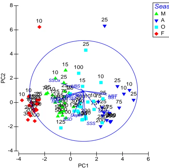
The variation of physical parameters was mainly explained by axe 1 of PCA with 41.7% (Fig 7). The PCA showed that this variation was resulted from a set of physical parameters such as SST and NBT and Secchi disk in increasing trend, and of SSD, NBD and SSOx in

decreasing trend. The second principal component, PCA2, explained such a variation with 19.1% and resulted mainly from a decreasing trend of SSD, SSS, and Depth.

(29)

28 A significant difference in SST and NBT was not observed among the transects (fig 8), with an exception of colder water in the station (T3_10) in front of Manavgat river, mostly in August and in February.

The February SST and NBT lightly increased from the shallow to deeper waters, passing from 19.7 to 20.5 °C and from 18.9 to 20.5°, respectively. On the contrary, these

temperatures decreased from inshore to offshore in August, passing from 27.6 to 25.2°C (SST) and from 27.6 to 24.6°C (NBT). In May and in October the temperatures were no significantly different.

Figure 7 Principal Component analysis (PCA) of physical parameters of Antalya gulf.

-4 -2 0 2 4 6 PC1 -4 -2 0 2 4 6 8 P C 2

Season

M A O F 10 25 75 125 200 300 10 ₇₅25 125 200 10 25 75 125 200 300 65 30 15 50 100 10 25 75 125 200₃₀₀ 25 75 125 200 10 25 75 125 200300 10 25 75 125 200 30010 25 75 125 200 10 25 75 125 200₃₀₀ 5050 100 15 10 25 75 125 200 300 10 25 75 125 200 10 25 75 125 200 300 10 40 Depth STSMNBTSM Sechi SSOx NBOx SSTNBT SSS NBS SSD NBD

(30)

29 Figure 8 Spatio-temporal distribution of sea surface (red) and near bottom temperature (blue) values

(⁰C). (Black numbers are depth in meters).

Salinity did not vary relevantly with depth, nevertheless some exception. Sea Surface Salinity of station in front of Manavgat river (T3_10) was significantly lower than other stations. The

May 2014

August 2014

October 2014

(31)

30 SSS of this station was 36.1 psu in May, 24.1 psu in August, 29 psu in October and 34.5 psu February. In May, SSS increased from inshore to offshore passing from 36.1 to 40.3 psu. However, NBS did not display this trend. In Figure 9, is shownthe very low SSS in May (33.9 psu) of the station close to Manavgat river (T3_10) . SSS in October and in August were homogeneous more among the depth, showing a small range between SSS and NBS for each station. Spatial distribution of salinity was similar to that of the temperatures in

February, but regarding salinity the range of differences was less than temperature, detecting a slight increase from inshore to offshore.

May 2014

August 2014

(32)

31 Figure 9 Spatio-temporal distribution of sea surface (red) and near bottom salinity (blue) values

(PSU). (Black numbers are depth in meters).

The Sea Surface Oxygen (SSOx) and Near Bottom Oxygen (NBOx) were significantly different among seasons and bottom depths, showing for each season a decreasing trend from coast seaward (fig 10). The SSOx reached the peak value in colder waters in May (9.24 for SSOx and 9.26 for NBOx) and February (9.84 for SSOx and 9.44 for NBOx) and it was significantly lower in August (7.46 for SSOx and 7.76 for NBOx).

February 2015

May 2014

(33)

32 Figure 10 Spatio-temporal distribution of sea surface (red) and near bottom oxygen (blue) values (mg L⁻₁). (Black numbers are depth in meters).

The Sea Surface Density (SSD) and Near Bottom Density (NBD) showed a decreasing trend from coast seaward (Figure 11). The density of the sampling station in front of Manavgat river was very low compared to the others (Figure 11). Although the density patterns appeared to be more complex in October as compared with those of the other seasons, SSD decreased from 25.23 to 27.75 passing form the inshore waters to the offshore waters.

October 2014

(34)

33 Figure 11 Spatio-temporal distribution of sea surface (red) and near bottom density (blue) values

(sigma-t). (Black numbers are depth in meters).

May 2014

August 2014

October 2014

(35)

34

3.2 Distribution of diversity

The four surveys in the Antalya Gulf allowed the sampling of 58 crustacean species

belonging to three orders (Stomatopoda, Isopoda and Decapoda) and NN families. Eighteen species were non native species (table 3).

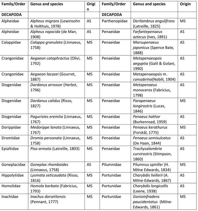
Table 3 Crustacean species collected from Antalya Gulf, with order and family, and with their origin (MS: Mediterranean Sea; AS: Alien Species).

Family/Order Genus and species Origi n

Family/Order Genus and species Origin

DECAPODA DECAPODA

Alpheidae Alpheus migrans (Lewinsohn

& Holthuis, 1978)

AS Parthenopidae Derilambrus angulifrons

(Latreille, 1825)

MS Alpheidae Alpheus rapacida (de Man,

1908)

AS Penaeidae Farfantepenaeus aztecus (Ives, 1891)

AS Calappidae Calappa granulata (Linnaeus,

1758)

MS Penaeidae Marsupenaeus

japonicus (Spence Bate,

1888)

AS

Crangonidae Aegaeon cataphractus (Olivi,

1792)

MS Penaeidae Metapenaeopsis

aegyptia (Galil & Golani,

1990)

AS

Crangonidae Aegaeon lacazei (Gourret,

1887)

MS Penaeidae Metapenaeopsis m.

consobrina(Nobili, 1904)

AS Diogenidae Dardanus arrossor (Herbst,

1796)

MS Penaeidae Metapenaeus

monoceros (Fabricius,

1798)

AS

Diogenidae Dardanus calidus (Risso,

1827)

MS Penaeidae Parapenaeus longirostris (Lucas,

1846)

MS

Diogenidae Paguristes eremita (Linnaeus,

1767)

MS Penaeidae Penaeus hathor

(Burkenroad, 1959)

AS Dorippidae Medorippe lanata (Linnaeus,

1767)

MS Penaeidae Penaeus kerathurus

(Forskål, 1775)

MS Dromiidae Dromia personata (Linnaeus,

1758)

MS Penaeidae Penaeus semisulcatus

(De Haan, 1844)

AS Epialtidae Pisa armata (Latreille, 1803) MS Penaeidae Trachysalambria

curvirostris (Stimpson,

1860)

AS

Goneplacidae Goneplax rhomboides (Linnaeus, 1758)

AS Pilumnidae Pilumnus spinifer (H. Milne Edwards, 1834)

MS Hippolytidae Lysmata seticaudata (Risso,

1816)

MS Portunidae Charybdis hellerii (A.

Milne-Edwards, 1867)

AS Homolidae Homola barbata (Fabricius,

1793)

MS Portunidae Charybdis longicollis

(Leene, 1938)

AS Inachidae Inachus dorsettensis

(Pennant, 1777)

MS Portunidae Gonioinfradens paucidentatus

(Milne-Edwards, 1861)

(36)

35 Inachidae Macropodia longirostris

(Fabricius, 1775)

MS Portunidae Liocarcinus depurator

(Linnaeus, 1758)

MS Inachidae Macropodia tenuirostris

(Leach, 1814)

MS Portunidae Portunus hastatus

(Linnaeus, 1767)

MS Latreillidae Latreillia elegans (Roux,

1830)

MS Portunidae Portunus pelagicus

(Linnaeus, 1758)

AS Leucosiidae Ixa monodi (Holthuis, 1956) AS Portunidae Thalamita poissonii

(Audouin, 1826)

AS Majidae Maja goltziana (d’Oliveira,

1888)

MS Processidae Processa edulis (Risso,

1816)

MS Majidae Maja squinado (Herbst, 1788) MS Sicyoniidae Sicyonia lancifer (Olivier,

1811)

AS Paguridae Anapagurus chiroacanthus

(Lilljeborg, 1856)

MS Solenoceridae Solenocera

membranacea (Risso,

1816)

MS

Paguridae Anapagurus petiti (Dechancé

& Forest, 1962)

MS ISOPODA Paguridae Pagurus alatus (Fabricius,

1775)

MS Aegidae Rocinela dumerilii

(Lucas, 1849)

MS Paguridae Pagurus excavatus (Herbst,

1791)

MS Cymothoidae Cerotothoa oestroides

(Risso, 1816)

MS Paguridae Pagarus prideaux (Leach,

1815)

MS Cymothoidae Nerocila bivittata (Risso,

1816)

MS Palinuridae Palinurus elephas (Fabricius,

1787)

MS STOMATOPODA Pandalidae Chlorotocus crassicornis (A.

Costa, 1871)

MS Parasquillidae Parasquilla ferussaci

(Roux, 1828)

MS Pandalidae Plesionika edwardsii (Brandt,

1851)

MS Squillidae Erugosquillamassavensi s (Kossmann, 1880)

AS Pandalidae Plesionika heterocarpus (A.

Costa, 1871)

MS Squillidae Squilla mantis

(Linnaeus, 1758)

MS

The annual distribution of dominance (D), the frequency of occurrence (FO)and the numerical occurrence of the crustacean species were given in table 4.

Looking the annual dominance, no constant species were found in the study area,

nevertheless some crustacean species were identified as common in the area. The most dominant species were Pagurus prideaux (Leach, 1815) and Parapenaeus longirostris (Lucas, 1846) both occurring in 38.46% of stations with a frequency of occurrence of 7.83%. These were followed by Charybdis longicollis (Leene, 1938) that occurred in 33.33 % of stations (FO = 6.79%) and Marsupenaeus japonicus (Spence Bate, 1888) that occurred in 26.92% of stations (FO = 5.48%). Most of the species were considered rare and 10 species were very rare, summing up at 17.25% of total species and being recorded only in a few stations (D% 1.28% and FO 0.26%).

(37)

36 Table 4. Annual distribution of dominance (D in %), frequency of occurrence (FO in %), numerical

occurrence for abundance (NO1 in %), for biomass (NO2 in %) percentageofcrustacean species.

O rd er /S p ec ie s D % MA Y FO % MA Y N O 1 % MA Y N O 2 % MA Y D % A U G FO % A U G N O 1% A U G N O 2 % A U G D % O CT FO % O CT N O 1% O CT N O 2 % O CT D % F EB FO % F EB N O 1 % F EB N O 2 % F EB D % Y EA R FO % Y EA R N O 1 % Y EA R N O 2 % Y EA R D e ca p o d a A e ga e o n c ata p h ra ctu s 13 .6 4 3. 06 0. 04 0. 34 6. 25 2. 33 0. 03 0. 14 23 .8 1 3. 82 0. 17 0. 99 5. 26 0. 90 0. 02 0. 10 12 .8 2 2. 61 0. 09 0. 52 A e ga e o n la ca ze i 0 0 0 0 0 0 0 0 0 0 0 0 5. 26 0. 90 0. 13 0. 70 1. 28 0. 26 0. 02 0. 13 A lp h e u s mi gr an s 0 0 0 0 0 0 0 0 0 0 0 0 5. 26 0. 90 0. 00 0. 12 1. 28 0. 26 0. 00 0. 02 A lp h e u s ra p ac id a 0 0 0 0 0 0 0 0 4. 76 2 0. 76 3 0. 03 1 0. 03 8 0 0 0 0 1. 28 0. 26 0. 01 0. 01 A n ap ag u ru s ch ir o ac an th u s 0 0 0 0 0 0 0 0 0 0 0 0 5. 26 0. 90 0. 01 0. 12 1. 28 0. 26 0. 00 0. 02 A n ap ag u ru s p e ti ti 0 0 0 0 0 0 0 0 4. 76 0. 76 0. 05 0. 19 5. 26 0. 90 0. 01 0. 15 2. 56 0. 52 0. 02 0. 10 Ca la p p a gr an u la ta 18 .1 8 4. 08 2. 39 0. 18 12 .5 0 4. 65 7. 53 0. 26 19 .0 5 3. 05 4. 40 0. 22 10 .5 3 1. 80 15 .3 0 0. 56 15 .3 8 3. 13 6. 04 0. 28 Ch ar yb d is h e ll e ri i 0 0 0 0 0 0 0 0 0 0 0 0 10 .5 3 1. 80 0. 97 0. 44 2. 56 0. 52 0. 18 0. 09 Ch ar yb d is lo n gi co ll is 36 .3 6 8. 16 4. 42 3. 63 12 .5 4. 65 2. 22 1. 16 42 .8 6 6. 87 18 .9 9 13 .7 7 36 .8 4 6. 31 4. 79 3. 26 33 .3 3 6. 79 10 .1 6 7. 17 Ch lo ro to cu s cr as si co rn is 4. 55 1. 02 0. 02 0. 16 0 0 0 0 9. 52 1. 53 0. 03 0. 26 5. 26 0. 90 0. 01 0. 08 5. 13 1. 04 0. 02 0. 17 D ar d an u s ar ro ss o r 18 .1 8 4. 08 0. 27 0. 44 0 0 0 0 4. 76 0. 76 0. 03 0. 09 10 .5 3 1. 80 0. 07 0. 15 8. 97 1. 83 0. 11 0. 20 D ar d an u s ca li d u s 0 0 0 0 6. 25 2. 33 0. 18 0. 15 4. 76 0. 76 0. 08 0. 05 0 0 0 0 2. 56 0. 52 0. 05 0. 04 D e ri la mb ru s an gu li fr o n s 18 .1 8 4. 08 0. 32 0. 34 25 9. 30 0. 93 1. 05 23 .8 1 3. 82 0. 15 0. 34 21 .0 5 3. 60 0. 48 0. 88 21 .7 9 4. 44 0. 34 0. 52 D ro mi a p e rs o n ata 9. 09 2. 04 0. 23 0. 09 0 0 0 0 9. 52 1. 53 0. 19 0. 50 10 .5 3 1. 80 0. 19 0. 20 7. 69 1. 57 0. 18 0. 26 Fa rf an te p e n ae u s az te cu s 9. 09 2. 04 1. 16 0. 31 6. 25 2. 33 0. 67 0. 14 38 .1 0 6. 11 6. 83 1. 49 10 .5 3 1. 80 1. 83 0. 23 16 .6 7 3. 39 3. 52 0. 73 G o n e p la x rh o mb o id e s 4. 55 1. 02 0. 01 0. 05 0 0 0 0 9. 52 1. 53 0. 03 0. 25 0 0 0 0 3. 85 0. 78 0. 01 0. 11 G o n io in fr ad e n s p au ci d e n ta tu s 0 0 0 0 0 0 0 0 4. 76 0. 76 0. 04 0. 04 0 0 0 0 1. 28 0. 26 0. 02 0. 01 H o mo la b ar b ata 27 .2 7 6. 12 0. 31 0. 94 0 0 0 0 9. 52 1. 53 0. 02 0. 09 21 .0 5 3. 60 0. 32 1. 08 15 .3 8 3. 13 0. 16 0. 54 In ac h u s d o rs e tt e n si s 22 .7 3 5. 10 0. 07 0. 33 0 0 0 0 0 0 0 0 15 .7 9 2. 70 0. 04 0. 33 10 .2 6 2. 09 0. 03 0. 17 Ix a mo n o d i 0 0 0 0 12 .5 4. 65 0. 21 0. 33 4. 76 0. 76 0. 00 0. 03 5. 26 0. 90 0. 03 0. 12 5. 13 1. 04 0. 03 0. 07 La tr e il li a e le ga n s 4. 55 1. 02 0. 00 0. 03 0 0 0 0 0 0 0 0 10 .5 3 1. 80 0. 01 0. 38 3. 85 0. 78 0. 00 0. 08 Li o ca rc in u s d e p u ra to r 0 0 0 0 18 .7 5 6. 98 0. 74 1. 71 9. 52 1. 53 0. 04 0. 07 10 .5 3 1. 80 0. 08 0. 15 8. 97 1. 83 0. 10 0. 23 Ly sma ta s e ti ca u d ata 0 0 0 0 0 0 0 0 4. 76 0. 76 0. 01 0. 12 0 0 0 0 1. 28 0. 26 0. 00 0. 05 M ac ro p o d ia lo n gi ro str is 9. 09 2. 04 0. 04 0. 75 0 0 0 0 0 0 0 0 10 .5 3 1. 80 0. 01 0. 20 5. 13 1. 04 0. 02 0. 28 M ac ro p o d ia te n u ir o str is 4. 55 1. 02 0. 01 0. 12 6. 25 2. 33 0. 01 0. 18 4. 76 0. 76 0. 00 0. 04 10 .5 3 1. 80 0. 01 0. 17 6. 41 1. 31 0. 01 0. 10 M aj a go ltz ia n a 9. 09 2. 04 0. 22 0. 09 0 0 0 0 0 0 0 0 5. 26 0. 90 0. 15 0. 10 3. 85 0. 78 0. 10 0. 05 M aj a sp . 0 0 0 0 6. 25 2. 33 0. 08 0. 18 4. 76 0. 76 0. 02 0. 05 0 0 0 0 2. 56 0. 52 0. 01 0. 04 M aj a sq u in ad o 0 0 0 0 6. 25 2. 33 4. 09 0. 25 19 .0 5 3. 05 4. 56 0. 34 5. 26 0. 90 3. 26 0. 23 7. 69 1. 57 2. 83 0. 20 M ar su p e n ae u s ja p o n ic u s 13 .6 4 3. 06 2. 53 0. 52 6. 25 2. 33 4. 06 0. 70 23 .8 1 3. 82 6. 65 4. 20 42 .1 1 7. 21 18 .7 0 4. 93 21 .7 9 4. 44 7. 27 2. 79 M e d o ri p p e la n ata 36 .3 6 8. 16 3. 02 1. 54 18 .7 5 6. 98 1. 65 1. 16 23 .8 1 3. 82 0. 76 0. 62 26 .3 2 4. 50 1. 58 1. 30 26 .9 2 5. 48 1. 71 1. 10 M e ta p e n ae o p si s ae gy p ti a 4. 55 1. 02 0. 01 0. 04 0 0 0 0 14 .2 9 2. 29 3. 58 7. 45 10 .5 3 1. 80 0. 14 0. 47 7. 69 1. 57 1. 47 2. 95 M e ta p e n ae o p si s mo gi e n si s co n so b ri n a 0 0 0 0 0 0 0 0 4. 76 0. 76 0. 01 0. 04 5. 26 0. 90 0. 02 0. 05 2. 56 0. 52 0. 01 0. 02 M e ta p e n ae u s mo n o ce ro s 4. 55 1. 02 0. 08 0. 04 0 0 0 0 4. 76 0. 76 0. 03 0. 03 5. 26 0. 90 0. 29 0. 07 3. 85 0. 78 0. 09 0. 04 P ag u ru s al atu s 0 0 0 0 0 0 0 0 0 0 0 0 5. 26 0. 90 0. 04 0. 09 1. 28 0. 26 0. 01 0. 02 P ag u ru s e xc av atu s 13 .6 4 3. 06 0. 68 2. 22 0 0 0 0 4. 76 0. 76 0. 01 0. 04 21 .0 5 3. 60 0. 37 0. 76 10 .2 6 2. 09 0. 29 0. 87 P ag ar u s p ri d e au x 40 .9 1 9. 18 5. 25 11 .9 1 25 9. 30 4. 59 15 .0 2 61 .9 0 9. 92 6. 21 23 .0 2 21 .0 5 3. 60 7. 56 23 .4 7 38 .4 6 7. 83 5. 99 18 .7 0 P ag u ru s sp . 0 0 0 0 0 0 0 0 4. 76 0. 76 0. 24 1. 00 0 0 0 0 1. 28 0. 26 0. 10 0. 38 P ag u ri ste s e re mi ta 4. 55 1. 02 0. 01 0. 08 0 0 0 0 4. 76 0. 76 0. 01 0. 05 0 0 0 0 2. 56 0. 52 0. 00 0. 04 P ar ap e n ae u s lo n gi ro str is 31 .8 2 7. 14 69 .7 1 66 .1 9 43 .7 5 16 .2 8 71 .1 1 69 .6 6 42 .8 6 6. 87 29 .0 0 32 .0 2 36 .8 4 6. 31 20 .4 8 44 .7 3 38 .4 6 7. 83 44 .4 7 49 .3 8 P e n ae u s h ath o r 4. 55 1. 02 0. 43 0. 09 0 0 0 0 19 .0 5 3. 05 4. 38 2. 40 36 .8 4 6. 31 4. 90 1. 99 15 .3 8 3. 13 2. 79 1. 33 P e n ae u s ke ra th u ru s 4. 55 1. 02 0. 57 0. 08 6. 25 2. 33 0. 45 0. 29 14 .2 9 2. 29 1. 67 0. 65 0 0 0 0 6. 41 1. 31 0. 90 0. 30 P e n ae u s se mi su lc atu s 0 0 0 0 12 .5 4. 65 0. 36 0. 30 19 .0 5 3. 05 3. 00 0. 58 26 .3 2 4. 50 11 .0 3 1. 57 14 .1 0 2. 87 3. 25 0. 56 P il u mn u s sp in if e r 0 0 0 0 0 0 0 0 0 0 0 0 5. 26 0. 90 0. 00 0. 08 1. 28 0. 26 0. 00 0. 01 P is a ar ma ta 31 .8 2 7. 14 0. 27 0. 77 6. 25 2. 33 0. 04 0. 19 23 .8 1 3. 82 0. 18 0. 90 21 .0 5 3. 60 0. 84 3. 03 21 .7 9 4. 44 0. 31 1. 19 P le si o n ik a e d w ar d si i 4. 55 1. 02 2. 67 1. 41 6. 25 2. 33 0. 46 2. 77 9. 52 1. 53 1. 65 3. 23 10 .5 3 1. 80 0. 15 0. 79 7. 69 1. 57 1. 58 2. 13 P le si o n ik a h e te ro ca rp u s 9. 09 2. 04 0. 83 6. 75 0 0 0 0 4. 76 0. 76 0. 03 0. 30 15 .7 9 2. 70 0. 70 4. 09 7. 69 1. 57 0. 40 3. 07 P o rtu n u s h as ta tu s 0 0 0 0 0 0 0 0 4. 76 0. 76 0. 32 0. 08 5. 26 0. 90 0. 33 0. 33 2. 56 0. 52 0. 19 0. 09 P o rtu n u s p e la gi cu s 9. 09 2. 04 3. 76 0. 10 0 0 0 0 4. 76 0. 76 4. 92 0. 15 5. 26 0. 90 2. 93 0. 12 5. 13 1. 04 3. 71 0. 11 P ro ce ss a e d u li s 0 0 0 0 0 0 0 0 4. 76 0. 76 0. 02 0. 16 0 0 0 0 1. 28 0. 26 0. 01 0. 06 Si cy o n ia la n ci fe r 0 0 0 0 0 0 0 0 4. 76 0. 76 0. 02 0. 05 5. 26 0. 90 0. 06 0. 13 2. 56 0. 52 0. 02 0. 04 So le n o ce ra me mb ra n ac e a 0 0 0 0 0 0 0 0 9. 52 1. 53 0. 04 0. 21 5. 26 0. 90 0. 09 0. 23 3. 85 0. 78 0. 03 0. 13 Th al ami ta p o is so n ii 0 0 0 0 12 .5 0 4. 65 0. 50 4. 08 9. 52 1. 53 0. 56 2. 60 15 .7 9 2. 70 0. 29 0. 91 8. 97 1. 83 0. 33 1. 59 Tr ac h ys al amb ri a cu rv ir o str is 0 0 0 0 12 .5 0 4. 65 0. 11 0. 30 9. 52 1. 53 0. 12 0. 55 0 0 0 0 5. 13 1. 04 0. 06 0. 24 P h yl lo so ma P al in u ru s e le p h as 0 0 0 0 0 0 0 0 4. 76 0. 76 0. 02 0. 10 0 0 0 0 1. 28 0. 26 0. 01 0. 04 Iso p o d a Ce ro to th o a o e str o id e s 0 0 0 0 0 0 0 0 4. 76 0. 76 0. 01 0. 16 0 0 0 0 1. 28 0. 26 0. 00 0. 06 N e ro ci la b iv itt ata 0 0 0 0 0 0 0 0 0 0 0 0 5. 26 0. 90 0. 07 0. 28 1. 28 0. 26 0. 01 0. 05 R o ci n e la d u me ri li i 4. 55 1. 02 0. 01 0. 03 0 0 0 0 0 0 0 0 5. 26 0. 90 0. 03 0. 12 2. 56 0. 52 0. 01 0. 03 St o m at o p o d a Er u go sq u il la ma ss av e n si s 18 .1 8 4. 08 0. 69 0. 43 0 0 0 0 14 .2 9 2. 29 0. 40 0. 36 10 .5 3 1. 80 1. 70 0. 72 11 .5 4 2. 35 0. 69 0. 42 P ar as q u il la f e ru ss ac i 0 0 0 0 0 0 0 0 4. 76 0. 76 0. 02 0. 04 0 0 0 0 1. 28 0. 26 0. 01 0. 02 Sq u il la ma n ti s 0 0 0 0 0 0 0 0 9. 52 1. 53 0. 48 0. 07 0 0 0 0 2. 56 0. 52 0. 19 0. 03

(38)

37 3.2.1 Distribution of number of species

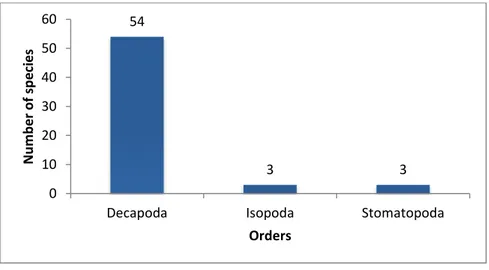
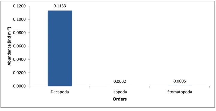
Three orders of Crustacea were observed (Fig 12). Decapoda showed the highest species number (54) follow by Stomatopoda order and Isopoda order (both with 3 species ).

Figure 12 Number of species of each order of Crustacea

Twenty-four families belonging to Decapoda were found (fig 13). The richest families in number of species collected were Penaeidae and Portunidae, respectively with 10 and 7 species. These were followed by Paguridae family with 6 species. In the family Portunidae, Charybdis longicollis was the most dominant species (33.33%) with a frequency of

occurrence was 6.79%.

The family Majidae was represented by 3 species, where the most frequent was the

commercial crab Maja squinado with a frequency of occurrence of 1.57%. Furthermore, 15 families were composed of only one species each, and among these Medorippe lanata (Linnaeus, 1767; Dorippidae) was the most frequently observed (26.92%). Ten species of decapoda were observed in a low frequency (0.26 % for each).

54 3 3 0 10 20 30 40 50 60

Decapoda Isopoda Stomatopoda

N u m b e r o f sp e ci e s Orders

(39)

38 Figure 13 Number of species of each family of Decapoda

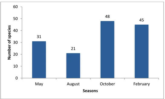
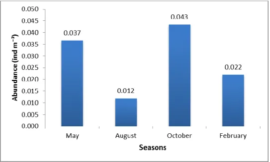
The number of species decreased from May to August, and then increased in colder seasons when it peaked the maximum value in October with 48 species. In February the number slightly decreased to 45 species (Fig 14) with lowest values registered in May (31) and in August (21).

Figure 15 showed the number of species for each order of Crustacea registered in each season.

Figure 14 Distribution of number of species of Crustacea in the seasons.

2 1 2 3 1 1 1 1 1 1 3 1 1 3 6 1 3 1 10 1 7 1 1 1 0 2 4 6 8 10 12 Alp h ei d ae Calap p id ae Cran gon id ae Diog en id ae Dorip p id ae Drom ida e Ep ialt id ae G o n e p lacid ae H yp p o ly tid ae H o m o lid ae In ach id ae La trei lli d ae Le u co sid ae Ma jid ae Pa gu rid ae Pa linu rid ae Pa n d al id ae Pa rth en o p id ae Pe n ae id ae Pilu m n id ae Po rtu n id ae Pro ce ss id ae Sic yo n iida e Sole n o ce rid ae N u m b e r o f sp e ci e s Families 31 21 48 45 0 10 20 30 40 50 60