Analysis of aircraft load spectrum by means of flight simulator

(1)

UNIVERSITA’ DI BOLOGNA

SCHOOL OF ENGINEERING AND ARCHITECTURE

Forlì Campus

Second Cycle Degree in

INGEGNERIA AEROSPAZIALE/ AEROSPACE ENGINEERING

Class LM-20

THESIS

in

Aerospace Structures

Analysis of aircraft load spectrum by means of

flight simulator

CANDIDATE

SUPERVISOR

Dario Donati

Enrico Troiani

Academic Year 2014/2015

Session II

(2)

Dedication

To my Father and Mother to whom I’ll be forever indebted.

(3)

Table of Figures

Figure 1: Typical S-N curve ... 10

Figure 2:Cyclic slip leads to crack nucleation ... 12

Figure 3: Fatigue life periods ... 13

Figure 4: Parameters for design against fatigue ... 16

Figure 5: Design on the edge of failure concept ... 17

Figure 6: Safe-life approach design ... 18

Figure 7:De Hallivand Comet, fuselage explosion ... 19

Figure 8:Example of fail-safe designed structure ... 20

Figure 9:Rear spar top chord failure under fail-safe design approach ... 22

Figure 10:Potential of infinite life of a structure designed under Damage tolerance approach ... 23

Figure 11: Damage tolerance inspection periods ... 24

Figure 12: Typical damage tolerance diagram: crack growth and residual strength diagram ... 24

Figure 13:Safe-life VS Damage tolerance design approach ... 25

Figure 14: Damage tolerance inputs and outputs ... 26

Figure 15: Aircraft design philosophy ... 27

Figure 16: Crack growth curve of a multiple path structure... 27

Figure 17: Minimum detectable and critical crack length ... 28

Figure 18: Elliptical hole in a flat plate ... 31

Figure 19: Example of Residual strength diagram with Feddersen interpolation ... 36

Figure 20: Maximum permissible crack length on residual strength diagram ... 36

Figure 21: Typical crack growth curve with design life H ... 37

Figure 22: Fracture mechanism concepts for Damage Tolerance analysis ... 39

Figure 23: Crack opening modes ... 40

Figure 24: Stress concentration factor concept ... 42

Figure 25: Stress concentration factor for different geometry notches ... 42

Figure 26: Infinite element at the crack tip ... 43

Figure 27: CTS specimen typically used for fracture toughness experiment test ... 48

Figure 28: Geometry factor curve ... 48

Figure 29: Fracture collapse VS plastic collapse ... 51

(6)

Figure 32: Fatigue crack growth regions ... 55

Figure 33: Crack growth prediction based on similarity principle ... 59

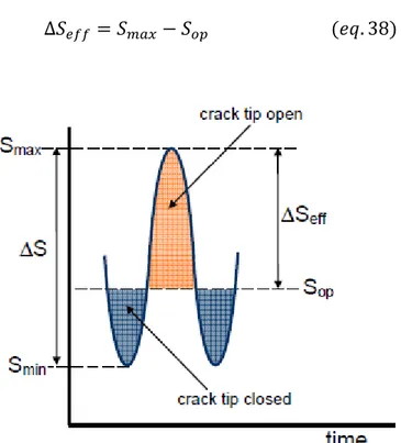
Figure 34: Elber's experiment results about crack closure phenomenon ... 62

Figure 35: Effective stress range ... 63

Figure 36: Crack tip opening ... 65

Figure 37: Crack growth retardation phenomenon ... 66

Figure 38: Thickness effect on retardation phenomena ... 66

Figure 39: Material Yield strength effect on retardation phenomena ... 67

Figure 40: Simple VA load sequence ... 67

Figure 41: Crack growth retardation due to overload ... 68

Figure 42: Yield zone model concept ... 72

Figure 43: Humps formation on crack surface due to overloads ... 76

Figure 44: Load sequence considered in PERFFAS model ... 78

Figure 45: Dugdale model ... 80

Figure 46: Equivalent schematization to Dugdale model ... 80

Figure 47: Rule of load spectrum in fatigue analysis procedure ... 81

Figure 48: Typical wing load spectrum per flight ... 82

Figure 49: Regular and symmetrical load history ... 84

Figure 50: Regular not-symmetric load history ... 85

Figure 51: Irregular load history ... 86

Figure 52: Level cross counting method ... 86

Figure 53: Typical exceedance diagram ... 87

Figure 54: Number of peaks per interval ... 87

Figure 55: Exceedance diagram for a non-symmetric load history ... 88

Figure 56: Difference between flat and steep load spectrum ... 89

Figure 57: 1D range counting method procedure ... 91

Figure 58: Typical 2D range counting matrix ... 92

Figure 59: Simple load sequence ... 93

Figure 60: Effect of intermedia small range ... 93

Figure 61: Cyclic plasticity loop ... 94

(7)

Figure 64: Basic idea behind the Endo Rainflow algorithm ... 96

Figure 65: Endo algorithm concept ... 96

Figure 66: Typical Semi-Random load sequence ... 98

Figure 67: Semi random Stress History generation ... 100

Figure 68: Accuracy variation with different number of load levels ... 101

Figure 69: FALSTAFF standardized loading sequence ... 103

Figure 70: TWIST standardized load sequence ... 104

Figure 71: Boeing C-17 Globemaster III ... 107

Figure 72: Euler and Aerodynamic angles ... 112

Figure 73: 3D Digital Datcom output ... 128

Figure 74: Typical outputs of Digital Datcom software ... 129

Figure 75: Root locus coming from design procedure used ... 139

Figure 76: General overview of the 6DOF flight dynamic model in Simulink environment ... 142

Figure 77: Non-linear equation of motion subsystem ... 143

Figure 78: ISA atmospheric model Simulink block ... 145

Figure 79: Gravity model Simulink block ... 146

Figure 80: Pitot tube representation for airspeed measurements ... 146

Figure 81: Barometric altimeter simulation for altitude measurements ... 147

Figure 82: Speed Variation ... 149

Figure 83: Altitude variation ... 149

Figure 84: Pitch angle comparison ... 149

Figure 85: Bank angle comparison ... 150

Figure 86: 2D trajectory tracked ... 150

Figure 87: 3D trajectory tracked ... 150

Figure 88: Automatic 2D trajectory tracked with RNP constrinments ... 151

Figure 89: 2D Trajectory tracked ... 151

Figure 90: 3D Trajectory tracked with RNP constrains ... 151

Figure 91: Cross track errors ... 152

Figure 92: Along track errors ... 152

Figure 93: Altitude error ... 152

(8)

Figure 96: Simple wing schematization ... 157

Figure 97: Inertial force time history ... 158

Figure 98: Lift force spectrum ... 159

Figure 99: Volume and contact forces on a generic body ... 160

Figure 100: Body interactions ... 163

Figure 101: Infinitesimal 3D material portion of tetrahedral shape ... 164

Figure 102: 2D infinitesimal material portion of tetraedic shape ... 165

Figure 103: Beam loads characteristic distributions ... 172

Figure 104: Double T section dimensions ... 174

Figure 105: Generated stress history ... 175

Figure 106: Stress history generated divided in levels ... 178

Figure 107: Exceedance diagram of the obtained stress history ... 180

Figure 108: Histogram representing number of peaks per interval ... 180

Figure 109: Summary table of the processed load spectrum ... 182

Figure 110: 2D Rainflow counting matrix ... 185

Figure 111: Testing constant amplitude load sequence ... 186

Figure 112: Testing damping load sequence ... 186

Figure 113: 2D Rainflow 2D counting matrix for CA testing loading sequence ... 187

Figure 114: Rainflow 2D counting matrix for damping testing load sequence ... 187

Figure 115: Critical locations for crack development ... 194

Figure 116: Residual strength diagram with Feddersen interpolation ... 195

Figure 117: Crack growth results from non-interaction model ... 199

Figure 118: Crack growth results from Yield zone model ... 201

Figure 119: Crack growth results from crack closure model ... 203

Figure 120: Time period H to reach critical crack length ... 205

Figure 121: Probability of detection curve ... 206

Figure 122: Different fracture control procedure ... 208

Figure 123: Fracture control for different crack growth process ... 209

Figure 124: Fracture control inspection interval prescribed ... 213

Figure 125: Different fracture control plan ... 214

(9)

Figure 128: Load characteristics related with elliptical lift distribution ... 225

Figure 129: Load characteristics related with triangular inertial force distribution ... 225

Figure 130: Part through crack and through crack ... 226

Figure 131: Semi-elliptical initial flaw extension ... 227

Figure 132: Stress intensity factor variation on the crack front of a semi-elliptical crack ... 229

Figure 133: Part through crack shape variation during crack extension ... 230

(10)

10

1 INTRODUCTION

What is fatigue?

Fatigue failures in metallic structures are a well-known phenomenon. The failures were already observed in 19𝑡ℎ century, and the first investigation on fatigue were carried out in that time by August Wohler. He recognized that, a single load application, far from the static strength of the structure, did not do any damage to the structure. However, if the same load was repeated many times, it could induce a complete failure. This observation conduced him to develop his famous S-N curve where the maximum applicable repeated stress as a function of the number of times that it can be applied before failure is represented.

Figure 1: Typical S-N curve

In the 19𝑡ℎ fatigue was thought to be a mysterious phenomenon in the materials because fatigue damage could not be seen. Failures apparently occurred without any previous warning. In the 20𝑡ℎ was learned that repeated load applications can start a fatigue mechanism in the material leading to nucleation of a microcrak, crack growth and ultimately to complete, failure of the structure. Understanding of the fatigue mechanism is essential for considering various technical conditions which affect fatigue life and fatigue crack growth. In fact, fatigue prediction methods can only be

(11)

11

evaluated if fatigue is understood as a crack initiation process followed by a crack growth period. For this reason, fatigue life is generally split in two different periods: crack initiation period and

crack growth period.

Fatigue process

The initiation period is supposed to include some microcracks growth but the fatigue cracks are still too small to be visible by eyes. In the second period, the crack is growing until complete failure.

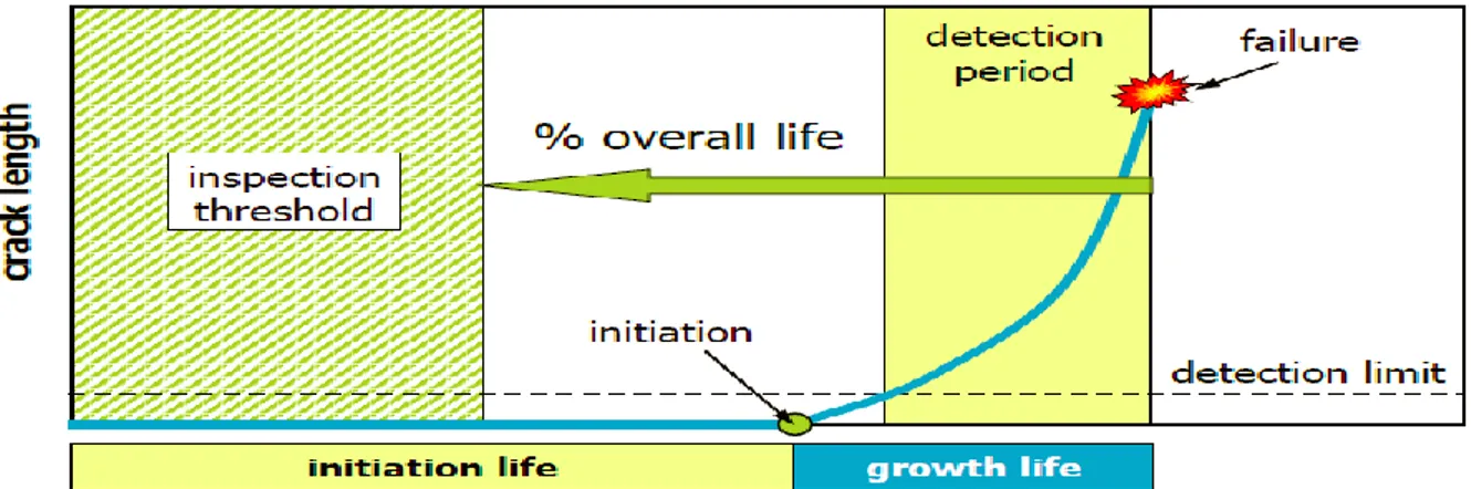
It is of significantly importance to split the fatigue life of a structural component in these two different periods and treat them separately. In fact, several practical conditions have a large influence on crack initiation period but only limited or, no influence at all, on crack growth period. Moreover, fatigue prediction methods are also different for the two periods. The stress concentration factor 𝐾𝑡 (Chapter 3) is the important parameter for predictions on crack initiation.

On the other hand, stress intensity factor 𝐾 (chapter 3) is the most important parameter to predict crack growth.

Nucleation of microcraks generally occurs very early in the fatigue life. It takes place almost immediately in the fatigue. However, fatigue failure does not occur if the applied loads are below the so called fatigue limit whose value is a function of the selected material and the applied mean stress. In spite of early crack nucleation, microcrak remains invisible for a considerable part of the total fatigue life. After a microcrack has been nucleated, crack growth can still be a slow and erratic process, due to the effects of the micro structure such as grain boundary. Deeper details about microscopic effects are out of the purpose of this work and for this reason they will not be described here in deep. More details about the fatigue process can be found in [1] Anyway, what is important to underline here, is that, once some microcrack growth has occurred away from the nucleation site, a more regular crack growth process is observed. This is the beginning of the second period introduced before. In few words, the crack initiation period and crack growth period can be described as follow:

1. Crack initiation period

Fatigue crack initiation, is a consequence of cyclic slip in slip bands. These cyclic slip requires cyclic shear stress. In particular, on a microscopic level, these shear stresses are not homogeneously

(12)

12

distributed through the material. In some grains at the material surface, especially due to the lower containment that is present because of at one side environment is present, condition for cyclic slip are more favourable. If a slip occurs in a surface grain, a slip step will be created at the material surface. It implies that a rim of new material is exposed to the environment. An important aspect, that probably is the key point of the fatigue process, is that, slip during the increase of the load also implies a strain hardening in the slip band. The consequence is that, upon unloading a larger shear stress, in the reverse direction, will be needed on the same slip band. For this reason reverse slip does not occur on the same slip band but on a parallel one. In fact, if cyclic slip would be a fully reversible process, fatigue phenomenon would not exist.

The following figure intends to summarize the general fatigue process during this firs period:

Figure 2:Cyclic slip leads to crack nucleation

As already mentioned, initiation period is a material surface phenomena.

2. Crack growth

This second period, related with a crack already propagated inside the material, is no longer a surface phenomenon but it is considered to be a bulk property of the material. In fact as will be introduced in following chapter, crack growth resistance is a characteristic of the typical material considered. How fast the crack will grow inside the material depends on the crack growth resistance of the material itself. It is generally expressed in term of crack growth rate, the crack length increment per cycle.

(13)

13

This quick introduction done up to now on the general fatigue process, can be summarized by the following figure.

Figure 3: Fatigue life periods

The second period is that one on which our work is focused. As will be discussed later on, crack growth relations are descried by the so called fracture mechanism concepts. All these concepts and their importance on modern design approach against fatigue failure will be presented later on in this thesis. Relations on which these concepts are based will not be mathematically derived in deep. In fact, a predicting engineering does not care about it, but it is accepted that it can be done. The real concern is what it means for the solution of practical problems.

Main purposes of this work

Design offices prefer standardized calculation procedures for predictions on fatigue strength, fatigue life, crack growth and residual strength. Standardized procedures can be useful, but it should be realized that such procedures may imply a considerable risk of unconservative or overconservative results. The main reason is that, such calculation procedures, start from some generalized conditions, which are not really similar to that of the problem. It then requires understanding, experience and engineering judgment to evaluate the significance of the calculated result. In case of some doubts about calculated predictions, it is useful to perform supporting fatigue tests. Some people in fact consider experiment as highly superior that theoretical calculation saying that “Experiment never fails”. It could be considered true but however, must be recognized that experiments can provide results applicable to the condition of the experiment only. This was not realized in the past and many accidents happened for this

(14)

14

reason. Also experiments require question about test condition and realistic service simulated condition so that they need understanding, experience and engineering judgment. In other words, all these observations are to say that, whether design against fatigue failure is done by analysis, calculation or experiments, it requires a profound knowledge of the fatigue phenomenon in a structure, material and the large variety of condition that can affect fatigue.

On the basis of this observation, the work developed on this thesis has the purpose to reduce standardized procedures used to design an aircraft against fatigue failure. As will be clear in the following, one important parameter needed to perform analysis about crack growth rate, on which modern design approach are based, is represented by service load spectrum. Service load spectrum for the structure to be used should be as much as possible similar to the real one at which the designed structure will be subjected. Today, in aeronautical design approach, standardized load sequences that will be introduced in Chapter 2 are one of the most common used methods to represent service load spectrum for the airplane to be designed. They are used because provide a quite economical way in term of money and time to proceed. However, these standardized load sequences could be in same case to much general for the specific design to be carried out. For this reason, the central focus of this work is the development of a numerical methodology to design an aircraft, against fatigue failure that, using load spectrum derived from an appositely designed flight simulator allowing to represent closely typical missions, providing the most important results of the modern damage tolerance approach using concepts provided by fracture mechanism. This way to proceed should provide results less general with respect those coming out from damage tolerance design approach using the standardized load sequences mentioned before.

The following of this thesis will be structured as follow: in chapter 2 the main approaches developed in the history of the design against fatigue are presented. Doing this will be pointed out many different accidents that were the starting point to improve current methodology to arrive at the modern damage tolerance approach. The basic concept on which this new design approach is based will be here in this chapter introduced. The basic one is represented by fracture mechanism. The main relation supporting fracture mechanism theory will be introduced and described in Chapter 3, they are fundamental to understand the different steps on which the numerical approach developed is based. In Chapter 4 the importance of load spectrum and how they can be processed will be described in deep. Here a description of the main standardized sequence commonly used today in aeronautical approach will be also described. Chapter 5 deals with the

(15)

15

designed flight dynamic simulator. Within this chapter the principal concepts needed to understand and use this one to produce specific load spectrum will be introduced in deep starting from the dynamic equation needed to represent forces and moments up to the control system used to manually and automatically flight the aircraft along predefined trajectories. Moreover all the principal blocks developed in Matlab/Simulink environment will be described. All the previous concepts will be then used in Chapter 6 to explain step by step the points followed to develop our methodology. The intent of our work is the development of a first methodology providing damage tolerance approach. For this reason in doing this, many assumptions have been introduced to simplify the problem. In this chapter all the assumptions introduced are described and explained so that, once this methodology has been tested and verified they can be removed to produce more real results.

(16)

16

2 EVOLUTION OF AIRCRAFT FATIGUE DESIGN

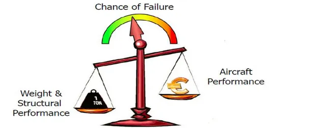
Over time, subjected to repeated service loading, the residual strength of the structure will decrease. The objective of designing against fatigue is to ensure that the residual strength remains above the design limit load for the useful life of the structure, through design or prescribed inspections.

Figure 4: Parameters for design against fatigue

Safe-life philosophy

In this type of approach, practise is to establish a finite life (safe life) based upon empirical data on the life of the structure until failure. In other words, the safe-life design products are designed to survive a specific “design life” with a chosen reserve. The infinite-life design, is a subset of the safe-life methodology where, operational stresses, are set to be below the fatigue limit of the material. This type of approach to design against fatigue failure, is generally employed in critical systems which are either, very difficult to repair or may cause severe damage to life and property. These types of systems are designed to work for years without requirement of any repairs.

(17)

17

Designing under this approach, the basic instrument to be used is the S-N curves generated for the specific element that we are going to design or coming out from tests on coupon elements of the same material but with different geometry. In fact, generally the S-N curves , are provided for a specific material but considering a simple rotating bending coupon (constant amplitude).

Especially in this second case, in which the S-N curve is based on coupons and not on samples of the structure, many different observations are needed before to use this one. Typical important questions that must be carried out designing under this approach are:

 How representative is the load on the coupon with respect to the load acting on the real structure in service?

 How comparable are the surface condition of the coupon and the real structure?

 Which are the environmental conditions used to make the tests on the coupon?

The answers at each of these questions are extremely important because, learning from the past, each of these parameters can strongly affect the fatigue life of a component in service.

For all these reasons (and many others!) a large amount of scatter is typically present in an S-N curve. Using safe-life design approach, scatter and uncertainties must be taken into account by using safety factor which could increase the weight of the structure without any need of this. Starting from these observations one can understand how, the principal drawback of structural elements designed under safe-life approach, is the fact that they are generally over-built with respect what is needed, which may be uneconomical. Of course, it is especially true in case where, an infinite-life design approach is used. This explains why, this particular design approach, is not practical for aerospace purpose. The following figure (figure 5) explains a quite clear concept about the problem of designing against fatigue in aerospace field.

(18)

18

This figure summarizes the needed to design on the edge of failure, typical of the aerospace field. Another drawback, designing under safe-life approach is that, once the design life is reached, the component must be substituted to maintain the designed safety even if it may still have a

considerable life ahead. A schematic visualization of the Safe-life design approach is available in the following figure.

Figure 6: Safe-life approach design

Safe-life design approach, also called finite-life design approach, has been applied in aerospace industry starting from the early 1950. Regulations, at that time, to design under this approach can be simply summarized as follow:

“The structure should be designed in so far as practicable, to avoid point of stress concentration where variable stresses above the fatigue design limit are likely to occur in normal service”

Summarizing, the two main tasks of a designer applying this methodology are:

1. Design so that stress levels are below the endurance limit everywhere in the structure 2. Retire the structure prior to the fatigue life

For this reason the main instrument needed to apply this methodology are:

 Wohler curve (or only fatigue limit in case of infinite-life approach)

 Load spectrum

 Miner rule

Regarding to aerospace industry, the first failure of airplanes designed under this approach happened in 1954 at the De Hallivand Comet. Here the inconvenient was related with a problem not detected during fatigue tests because of an unfortunate load sequence creating a retardation

(19)

19

effect (plasticity at the tip of the crack creating the so called crack closure phenomena) ,not known at that time, that was not present in the real structure because of a smaller load sequence. In particular, failure happens for explosive decompression of the fuselage. Fuselage was designed to maintain pressure of 8000ft at 40000ft. Safe-life approach used a design limit of 16000 flights or 10 years. However, as mentioned, the problem here was related with the load sequence used during fatigue test producing a plasticity effect (Chapter 3) beneficial from a fatigue life point of view. The front section of the fuselage was tested to 11psi while overpressure valve in service was set to 8.5psi. Plastic deformation at defects ( n particular failure happened from defects at rivet hole) reduced stress raiser, resulting in 18000 cycles fatigue life. This problem was not known before.

Figure 7:De Hallivand Comet, fuselage explosion

Starting from 1959 Safe-life design approach was substitute by a newer approach, the so called

Fail-safe approach. However, Safe-life approach continues to be an option for particular elements.

Especially on helicopters, engines and undercarriages this design approach is still used in combination with fail-safe approach.

(20)

20 Fail-Safe philosophy

Here, the main concept is to ensure that, redundancies in a structure are present such that

obvious partial failure can be sustained. Designing under fail-safe approach means, in other words, design under a multiple stiffening elements concept. In this way, if one element fails, the load is redistributed and structure is still capable to carry loads safely. Anyway, redistribution of loads, once one element fails needs to be calculated in each case/failure. An example of a fail-safe system is reported in figure. It is a good example to understand the importance of recalculating the load distribution in each possible case/failure. In fact, as can be expected, loads redistribution on the system will be different in the case where the steel beam or the bronze beam fails.

Figure 8:Example of fail-safe designed structure

Significantly, a system’s being “fail safe”, does not means that failure is impossible/improbable to occur but rather that, system’s design, prevents or mitigate unsafe consequence of the system’s failure. That is, if and when a “fail safe” system fails, it is safe or at least no less safe than when it is operating correctly.

A key concept of this approach is that, a failure of a stiffeners, is easily detected and can be easily repaired or substituted. In fact, in fail-safe design approach is assumed that a complete element failure or partial failure would be obvious during a general area inspection and would be corrected within a very short time. The probability of detecting damage during routine inspections before it

(21)

21

could progress to catastrophic limits is very high. In other words, fail-safe design can be firstly seen as a safe-life design. In fact, also in this case, initially the structure is design to achieve a

satisfactory life with no significance damage. Then, in addition to the previous approach, structure is also designed to be inspectable in service and able to sustain significant and easily detectable damage before safety is compromised.

In aerospace industry, fail-safe approach has been applied starting from 1959. What is important to observe at this point is that, Paris relation (basic relation used today to design against fatigue as will be described in the following of this thesis) has been developed in 1960. It is an important observation because it underlines that, fail-safe design approach is not based on crack growth propagation. In fact, the previous mentioned inspections, on which this methodology is based, are not prescribed inspections but, on the other hand, they are simple routine inspections in which failure has an high probability to be discovered.

Regulation prescribed to design under fail-safe approach can be summarized as follow:

“It shall be shown by analysis/tests that catastrophic failure or excessive structural deformations are not probable after fatigue failure or obvious partial failure of Principle Structural elements (PSE). After such a failure, the remaining structure shall be capable of withstanding static loads corresponding with certain prescribed flight loading condition”

Principal Structural Elements (PSE), named in this sentence, are defined as those elements which significantly contribute to carry flight, ground, and pressurization loads and whose failure could result in a catastrophic failure of the airplane.

The first failure of an airplane designed under this approach happened in 1977. It was a Boeing 707 who lost its right horizontal stabilizer due to a fatigue failure of the rear spar top chord after 47600 hours of flight and 16670 landing even if the Design Service Goal (DSG) of the designed airplane, i.e. the flight cycles or flight hours used in the design was 60000 flight hours and 20 years.

The aircraft had been maintained correctly to an approved maintenance program but inspections methods and maintenance programs prescribed by the fail-safe design approach were inadequate to detect partial cracks. Following failure of the rear spar top chord, structure could not sustain loads long enough to enable detection of failure through inspections.

(22)

22

Figure 9:Rear spar top chord failure under fail-safe design approach

After this accident in 1978 there was the introduction of an additional regulation prescribing the increment of inspections for ageing aircraft

Damage Tolerance philosophy

Starting from 1980 recommendation for damage tolerance for large civil airplane was introduced. Damage tolerance can be seen as an extension of the concept of fail-safe.

The damage tolerance philosophy can be described as:

“The ability of structure to sustain anticipated loads in the presence of fatigue, corrosion or accidental damage until such damage is detected, through inspections or malfunctions, and repaired.”

Hence, the most important innovation, introduced by damage tolerance philosophy is that, during the design phase, damage is considered to occur and this damage will be associated with a reduction of strength over time. For this reason, a detection window, based on damage growth prediction, need to be define. This is the commonly used approach in aerospace engineering to manage the extension of cracks in a structure applying principles of fracture mechanism. This philosophy became the prevailing engineering philosophy after 1980, when a deeper knowledge about fracture mechanism was available. Before this time, redundancy approach, required by a fail-safe design, as described in the previous paragraph, was the prevalent method.

In a general way, the main task, designing under this design philosophy is to show that catastrophic failure, due to fatigue corrosion or accidental damage, will be avoided throughout the

(23)

23

operational life of the structure. In particular, this type of evaluation must be conducted for each part which could contribute to catastrophic failure such as wing, empennage, control surface and their systems, fuselage, landing gear and their primary structural elements (PSE). Each evaluation must include:

 Typical loading spectra, temperature and humidity expected during the operational life of the structure

 Identification of critical points (primary structural elements and detail design point), the failure of which, will cause a catastrophic failure of the aircraft

 Service history of airplanes with similar structures must be used in the evaluation

A structure can be considered damage tolerant if a maintenance program has been implemented. It will result in the detection and repair of accidental damage, corrosion and fatigue cracking before such damage reduces the residual strength of the structure below an acceptable limit. Damage tolerance philosophy, relies on three important capabilities that are the basic concepts of the fracture mechanism theory:

 Residual strength prediction

 Damage growth prediction

 Damage detection limits

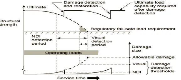
The basic idea behind this philosophy is that, when damage has been detected, it can be repaired and then, a new damage tolerance analysis must be performed to prescribe a new inspection window. Hence, inspections must be established as necessary to prevent catastrophic failure. Starting from this basic idea, this approach has the potential for an infinite life of the structure as shown in figure 10.

(24)

24

From performed damage tolerance analysis, designer can be able to determine an inspection threshold that can be considered as a safe-life for inspection, i.e. no inspections should be done during this period because crack is not visible (initiation period) . However, a detection interval must be prescribed before detection limit is reached. Within these inspection intervals,

inspections must be performed to monitor crack growth. The following figures (11,12) summarize all the concepts introduced up to know.

Figure 11: Damage tolerance inspection periods

(25)

25

Crack growth curve represented in figures above has been determined using the fracture mechanism analysis concepts which, as will be shown in the next chapter, are based on some material constants and a given service load spectrum coming out from structures already in service, working in a similar operational environment.

The following figure 13 makes more clear the improvement introduced by damage tollerance philosophy with respect to the first explained safe-life approach.

Figure 13:Safe-life VS Damage tolerance design approach

Again this figure shows how, during the initial life period of the component, no inspections are needed. Here, can also be seen clearer the fact that, in damage tolerance analysis, not only one inspection should be performed but many inspection intervals must be prescribed so that, when the crack is detected, structure is repaired with the positive consequence of increasing its

operation life ahead respect to its initial nominal life. As will be described in Chapter 6, inspection interval are prescribed using fracture control methods based on probability of detection. All the observations did up to now, make clear how this type of approach is beneficial from an

economical point of view.

With regard to the difference between Damage Tollerance philosophy and fail-safe approach, it can be explained in term of inspections required. In fact, while fail-safe as described before does not prescribe additional inspections to those of routine, confiding on a failure easily visible. On the other hand, Damage tolerance does not require consideration of complete failure or obvious partial element failure but it requires an inspection program tailored to the crack propagation characteristics of the particular part when subjected to the loading spectrum expected in service. This inspection program must be provided to ensure that cracks are detected before they reach a critical length (figure 12). Damage Tollerance places a much higher emphasis on inspections

(26)

26

needed to detect cracks before they progress to unsafe limits. Anyway as we will see in the following paragraph, fail-safe features may be included in structure designed to satisfy damage tolerance requirements.

The following figure, schematically represents all the input needed and the output achievable with a computer software performing damage tolerance analysis.

Figure 14: Damage tolerance inputs and outputs

This figure will result extremely useful in the following. In fact, it can be considered as a good visual summary of inputs and outputs of the methodology for the computer software damage tolerance analysis developed in our work. Details of how these inputs and outputs are obtained and their meaning is described in the next chapters of this thesis

Aircraft design philosophy

Today, designing an aircraft, all three methodologies described before are used. In particular, fail-safe approach is now used as a combination of pure fail-fail-safe and damage tolerance approach. It means that even if the structure is designed with a multiple path load approach, damage growth and inspections are still considered.

The following figure 15 shows a flow-chart representing the idea behind the use of all these methodologies to design an airplane.

(27)

27

Figure 15: Aircraft design philosophy

As can be expected from the introduction done up to now about each of these methodologies, the key question to distinguish when a safe- life or a fail-safe/damage-tolerance approach should be used is: Are inspections possible? Of course, cases in which inspections are not possible a safe-life approach must be used in spite of all its drawbacks introduced before. On the other hand, if inspections are possible, fail-safe/damage-tolerance approach must be used. Under this condition, difference between multiple load path structure and single load path structure must be

considered. In the first case the influence of the failure of each path on the crack growth on the others must be considered, in particular a reduction of the crack growth life (CGL) or, in the same way, an increase in the crack growth rate must be accounted for. A typical behaviour of the variation of the crack growth in a multiple load path structure when a path fails is represented in figure 16.

(28)

28

On the other hand, in case where a single path load structures is selected as design choice, a threshold should be based on crack growth analysis assuming maximum manufacturing defect size (Figure 17). Generally this type of parameter is provided in term of minimum allowable residual strength. Then, starting from this value, using fracture mechanism concepts and other

consideration related with plastic collapse the value of the critical crack length can be obtained. The way to proceed to get this value will be deeply described in the following of this thesis.

Figure 17: Minimum detectable and critical crack length

Input for Damage Tolerance Analysis

Before to introduce a list of the main inputs needed for damage tolerance analysis, which will be analysed in deeper detail in the following paragraphs, we need firstly to summarize which are the main assumptions and capabilities required for a damage tolerance analysis. They are a logic consequence of the basic concepts on which this type of philosophy is based.

A first important assumption is that, a significant proportion of the fatigue life up to failure is occupied by crack growth (remembering that as pointed out in Chapter 1, fatigue life of a structure can be divided in two periods: initialization period and crack growth period). A second important consideration is that, we need to be sure about damage detection and monitoring techniques which must have accuracy compatible with the rates of damage growth and damage influence on residual strength. It is a key point to be sure that detection can be

(29)

29

performed as it is prescribed. On the other hand, these detection techniques are based on the assumption that, predictive capability of damage growth rates and damage extent, are accurate enough to accurately calculate residual strength of damaged structure. Moreover, on the basis of production process, damage tolerance analysis relies on the ability to fabricate structures resistant to damage initiation and damage growth.

The list of inputs mentioned before, needed for the damage tolerance analysis, can be summarized with the following points:

 Service load spectrum for anticipated service environment. This spectrum must be typical of anticipated used. Today TWIST or MINITWIST (for transport aircraft) and FALSTAFF or short FALSTAFF (for military aircraft) are the standard spectrum used to initiate the damage tolerance analysis of the new structure to be designed. The effort of this thesis is to improve this point; generating more informative load spectra for the structure currently designed using an appositely developed flight simulator.

 Stress analysis measured relating with stresses to stresses at the crack site. Important will be consider here effect load sequence on crack growth (Chapter 3).

 Stress intensity factor from start defect size to failure

 Material crack growth rate data for selected material coming from handbook

 Predictive models for crack growth process.

Following of this thesis treats each of these points in deeper detail. In addition, in Chapter 6, they will be used to develop a methodology that, starting from data coming out from the already mentioned flight simulator (whose design is described in Chapter 5 ), used to get typical load spectrum, is able to perform a damage tolerance analysis.

(30)

30

3 FRACTURE MECHANISM

Historical Overview

Several structure failures can be associated with the fracture of one or more of the components making the structure. When such events occur, they are mostly unexpected, sudden and unfortunate, and it is natural to focus attention on minimizing the undesired consequences when designing and analysing modern-day structures. The study of crack behaviour, prevention and analysis of fracture of materials is known as fracture mechanism.

In other word fracture mechanism can be also defined as:

“The study of mechanical behaviour of cracked material subjected to an applied load”

In every discipline, including fracture mechanism, it is of critical importance to examine the historical antecedents. This is the reason why in the previous chapter, describing the history of the design approaches against fatigue, we did some examples of accidents occurred in aerospace field in the past years. People who tend to ignore the past are more prone to repeat mistake. Development in fracture mechanism concepts is quite a new idea.

By the end of the 19th century, the influence of crack on structure strength was widely appreciated but its nature and influence was still unknown. The first study was carried out by an Inglies, a research who observed that, the corner of an elliptical hole in a plate (Figure 18) feels the highest stress and, as the ellipse gets longer and thinner the stresses at the corner become even larger. From his studies we got an estimation of the stress concentration factor at the tip of the corner that can be expressed as:

𝐾_𝑡 =𝜎𝑝𝑒𝑎𝑘 𝜎_𝑛𝑜𝑚 = 1 + 2 𝑎 𝑏 = 1 + 2√ 𝑎 𝜌 (𝑒𝑞. 1)

Where a and b are the semi-major and semi-minor axes respectively and ρ is the root radius at the tip of the ellipse. Deeper details on this relation and its influence in fracture mechanism will be analysed later on in this thesis.

(31)

31

Figure 18: Elliptical hole in a flat plate

Inglies evaluated various hole geometries and he realized that, it is not really the shape of the hole that maters but the length of hole perpendicular to the load and the curvature at the end of the hole.

The basic ideas leading to the start of the modern fracture mechanism can be attributed to a theory of fracture strength of a glass, which was published by A.A Griffith in 1920. Using Inglis’ work as foundation, Griffith proposed an energy balanced approach to study the fracture phenomenon in cracked bodies. A great contribution to the ideas about breaking strength of materials emerged when Griffith suggested that the weakening of material by a crack could be treated as an equilibrium problem. He proposed that the reduction in strain energy of a body when the crack propagates could be equated to the increase in surface energy due to the increase in surface area. The Griffith theory assumed that the fracture strength was limited by existence of initial cracks and that brittle materials contain elliptical microcracks, which introduce high stress concentration near their tips. He developed a relationship between crack length (a), surface energy connected with traction free crack surface (𝛾) and applied stress, which is given by:

𝜎2 =2𝛾𝐸 𝜋𝑎

(32)

32

Plasticity effects in metals limited the theorem and it was not discovered until Irwin’s work in 1948, when a modification was made to Griffith’s model to make it applicable to metals. Irwin’s first major contribution was to extend the Griffith approach to metals including their energy dissipated by local plasticity flow.

It is an interesting fact and pherpas relevant to point out that scientific curiosity towards fracture mechanism became significantly important engineering discipline after the unfortunate failures of Liberty ships during World War II. The Liberty ships were built used a new construction method for mass production in which the hull was welded instead of riveted. The Liberty ship program was an astounding success until 1943, when a Liberty ship broke completely in two while sailing in the North Pacific. An investigation into Liberty ship failures pointed out poor toughness of steel and transition from ductile to brittle behaviour at the service temperatures that ship experienced. It was noticed that the fractures initiated at the square hatched corners on the deck where there was a local stress concentration and the sharp corners acted like starter crack. Research into this problem was led by George Rankine Irwin. It was the research during this period that resulted in the development and definition of what we now refer to as Linear-Elastic-fracture-mechanism (LEFM). A major step ahead, occurred in 1950 when Irwin provided the extension of Griffith theory for an arbitrary crack and proposed the criteria for the growth of this crack. The criterion was that the strain energy release rate (G) must be larger than the critical work (Gc), which is required to create a new unit crack area. Irwin also related strain energy release rate to the stress field at the crack tip. In particular Irwin showed that the stress field in the area of the crack tip is completely determined by a quantity K called the Stress Intensity Factor K. In particular Irwin presented a relation between the energy release rate and the stress intensity factor as:

𝜎𝑖𝑗 =

𝐾𝑓_𝑖𝑗(𝛳)

√2𝜋𝑟 (𝑒𝑞. 2) 𝐾2 = 𝐸𝐺 (𝑒𝑞. 3)

Other scenarios of failures that were experienced during that period was that of the De Hallivand “Comet” commercial aircraft, already introduced in the previous chapter as a key point to pass from the safe-life design approach to a life-safe design approach against fatigue. The failure of this airplane was at that time analysed using the basic concept available of fracture mechanism. In particular, the equilibrium concept showed that the comparison between the critical energy

(33)

33

release rate and the energy release rate has not been large enough to prevent crack propagation in the failure of the commercial aircraft.

In 1960, a significant contribution to the development of LEFM was put forth when Paris advanced an idea to apply fracture mechanism principles to fatigue crack growth. Although he provides convincing experimental and theoretical arguments for his approach, the initial resistance to his work was intense and he could not find a peer-rewind technical journal to publish his manuscript. He finally opts to publish his work in a University of Washington periodical entitled “The Trend in Engineering”.

The Paris’s work was a landmark in the fatigue aspects of fracture mechanism and yields the equation:

𝑑𝑎

𝑑𝑁= 𝐶∆𝐾

𝑚_{(𝑒𝑞. 4)}

Where C and m are material constant parameters fitting the experimental curve results. This is the basic equation on which modern crack growth model used for damage tolerance analysis are based.

Linear elastic fracture mechanism is not valid when significant plastic deformation precedes failure.

The use of fracture mechanism and its main objectives

Fracture control of structures is the concerted effort by designers, metallurgist, production and maintenance engineers and inspectors to ensure safe operations without catastrophic fracture failures. Of the various structural failure modes (buckling,fracture,excessive plastic deformation) fracture is only one. Very often a fracture occurs due to an unforeseen overload on the undamaged structure. Usually, it is caused by a structural flaw or a crack: due to repeated or sustained “normal “ service loads a crack may develop (starting from a flaw or stress concentration) and grow slowly in size, due to the service loading. Cracks and defects impair the strength. Thus, during the continuing development of the considered crack, structural strength decreases until it becomes so low that the service load cannot be carried any more, and fracture

(34)

34

happens. Fracture control is intended to prevent fracture due to defects and cracks at the maximum load experienced during operation service.

If fracture is to be prevented, the strength should not drop below a certain safe value. This means that cracks must be prevented from growing to a size at which the strength would drop below the acceptable limit. In order to determine which size of crack is admissible, one must be able to calculate how the structural strength is affected by cracks especially as a function of their size. For this reason, one must first identify locations where cracks could develop. Analysis then must provide information on crack growth times and on structural strength as a function of crack size. These are the main purposes of this type of analysis called damage tolerance analysis.

As introduced in previous chapter, damage tolerance can be defined as the property of a structure to sustain defects or cracks. Elimination can be affected by repair or replacing of the cracked structure or component. In the design stage, one still has the options to select a more crack resistance material or improve the structural design to ensure that cracks will not become dangerous during the projection economic service life (Safe-life design approach). Alternatively, periodic inspections may be scheduled, so that, crack can be repaired or components replaced when cracks are detected. Either, the time for replacement or the inspections interval and type of inspection, must follow from the crack growth diagram calculated in the damage tolerance analysis.

Inspections can be performed by a number of non-destructive techniques, provided the structure is inspectable and accessible. Fracture control (Chapter 6) is a combination of measures such as described above, including analysis, to prevent fracture due to cracks during operation. It may include all or some of these measures, namely damage tolerance analysis, material selection, design improvement, possibly structural testing and maintenance/inspections/replacement schedules. The extent of the fracture control measures depends upon the critically of the component, upon the economic consequences of the structure being out of service, and last but not least, the consequential damage caused by a potential fracture failure. For example fracture control of a hammer may be as simple as selecting a material with sufficient fracture resistance but, on the other hand, fracture control of an airplane, includes damage tolerance analysis, tests and subsequent inspections and repair/replacement plans. Deeper observations on fracture control procedure will be introduced in Chapter 6.

Damage tolerance analysis and its results, as introduced in the previous chapter, form the basis of the fracture control plans. In fact, inspections, repairs and replacements must be scheduled based

(35)

35

on results coming out from a damage tolerance analysis. Mathematical tools employed in the damage tolerance analysis are fracture mechanism concepts. They provide equations used to determine how cracks grow and how crack affect the strength of the structure. These concepts and equations will be introduced in a deeper detail in the following paragraphs.

During the last 25 years fracture mechanism has evolved into a practical engineering tool. It is not perfect but no engineering analysis is. As an example of this imperfection, we can consider the relation used to determine bending stress

𝜎 =𝑀

𝐼 (𝑒𝑞. 5)

This relation, used also in our methodology, will be derivate in the following of this thesis but for the moment, what is interesting to note is that it is rather in error when used to calculated structural strength, because it ignores plastic deformation. Anyway it has been successfully used in fracture mechanism analysis in past years. In fact, what must be considered rather than the inadequacy of the concepts is the inaccuracies of the inputs, they have a large influence on the obtained results (Chapter 7). A deeper discussion about fracture mechanism will be carried out in the following of this chapter.

Naturally, results of damage tolerance analysis must be used judiciously, but this can be said of any other engineering analysis as well.

The observations introduced up to now, are just an introduction underlining the importance of fracture mechanism concepts, especially in the new design approach based on damage tolerance analysis. In particular, what comes out from all these considerations is that, the establishment of a fracture control plan requires knowledge of the structural strength, particularly as it is affected by cracks and time involved for cracks to grow to a dangerous size. Thus, fracture mechanism, that provides results for damage tolerance analysis, has two objectives:

 Determination of the effects of crack growth on strength (margin against fracture)

 Determination of crack growth as a function of time

Following figure (Figure 20) shows a general way of how the crack length affects the residual strength of the material. As will be well explained later on, this plot has been created considering the so called Feddersen interpolation needed to get physical results. In fact, results must consider

(36)

36

that the strength of the new free-crack structure has a finite (and not infinite!) residual strength (equal to the ultimate strength) and the residual strength, when the crack length is equal to the width of the structure, must be equal to zero.

These observations will be readdressed in detail later on in this thesis.

Figure 19: Example of Residual strength diagram with Feddersen interpolation

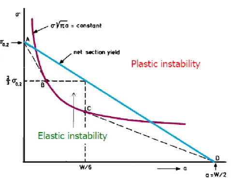
Due to continual growth, crack becomes longer and residual strength reduces. Probability of fracture will be higher. If nothing is done and the structure remains in service, residual strength at a certain point will become smaller than what is allowable so that fracture will occurs. This is what must be prevented: crack should not be allowed from becoming so large that fracture occurs at service loads. Hence the structure or component must be replaced before the crack becomes dangerous, or the crack must be detected and repaired before such time. In other words it means that some decision must be made to set the minimum permissible residual strength, so that, the maximum permissible crack size 𝑎𝑝 can be determined from the residual strength diagram.

(37)

37

Assuming that, minimum residual strength is provided, the maximum allowable crack size can be determined from a plot like that one in Figure 21. Even if the value of the minimum allowable residual strength is provided and from here the maximum allowable crack size can be directly determined, generally the calculation of the entire residual strength diagram is preferable. The residual strength diagram will be different no only for different structural components but it also depends on crack locations. It means that different maximum permissible crack size will be expected as well.

The maximum permissible crack size is generally called critical crack size. A critical crack is that one would cause fracture in service. Based on this definition, a crack will be critical only in the event that a stress larger the minimum residual strength occur.

Anyway knowing that the crack may not exceed 𝑎_𝑝 is of little help. For this reason, second objective of the fracture mechanism is to provide a crack growth curve representing the behaviour of crack length in time, generally expressed as number of cycles. A general crack growth curve is reported figure.

Figure 21: Typical crack growth curve with design life H

Under the action of normal service loading, cracks growth by fatigue, stress corrosion or creep. Starting at some crack size (a0) crack will grow in size during time with a typical behaviour reported in Figure 22. The permissible crack, is also plotted in a graph like that one before (Figure 22).

(38)

38

Still considering Figure 22, if a0 is for example an assumed initial defect, component or structure must be replaced after a certain time (expressed in number of cycle, hours or number of flight) named H. Since crack growth is not allowed beyond 𝑎𝑝, the crack must be detected and repaired

or otherwise eliminated before the time H has expired. Therefore, time between inspections must be less than H. For example doing an inspection at time t1 the crack will be missing being this one smaller than the minimum detection limit. So if the next inspection will be programmed H hours (or cycles or flights) later the crack would be reach the critical length 𝑎𝑝already which is not

permitted. For this reason a general inspection interval could be equal to H/2.

In any case the value of H comes out from damage tolerance analysis which also provides the residual strength diagram.

Fracture mechanism, as all engineering mechanism, uses stress rather than loads. Thus the residual strength diagram is generally expressed in term of stress and it represents the stress that the structure can sustain before fracture occurs. Residual strength should not be confused with residual stress that is the stress is rising in a structure while there are no loads applied. Also these types of stresses have a strong influence in fatigue life of the considered component but their meaning is completely different.

Stress can be used as the basis for the analysis if there is a relationship between the applied stress and the process taking place at the crack tip. As the crack tip events are governed by the local stresses at the crack tip, it is required that the local crack tip stress be described as a function of the applied stress.

To get a better idea about all the concepts introduced up to know, regarding the application of the fracture mechanism concepts that will be deeper considered later on, the following flow-chart (Figure 18) can be used to summarize visually the main steps needed to perform this analysis

(39)

39

Figure 22: Fracture mechanism concepts for Damage Tolerance analysis

Two of the most important concepts needed to track each of the charts of the previous flow chart are:

 Basic concepts and equations of the fracture mechanism

 Load spectrum

For this reason, before to deal with this flow chart, describing step-by-step the developed methodology to get a numerical damage tolerance analysis starting from load sequence generated using a developed flight simulator, the basic concepts and equations of fracture mechanism and the principal aspects of load spectrum and how they can be obtained to perform analysis must be quickly introduced so that the developed methodology will result more clear. Anyway what is

(40)

40

important to underline at this level of detail is that to derive these relationships one must distinguish between 3 modes of loading. They are shown in the following figure (Figure 24).

Figure 23: Crack opening modes

These modes of loading (no modes of cracking) are usually simply referred by Roman numerals as I,II,III. In a deeper detail they can be called as:

 Mode I: tension mode

 Mode II: in-plane shear mode

 Mode III: out-plane shear mode.

The crack tip stress equations are very similar for each of the modes and consequently the fracture and crack growth analysis. It is the reason why in the following of this thesis we will refer only to mode I (Tensile mode) being also the most common one. Note that, however, in reality, these modes do not occur individually but they generally occur in combination. This consideration will be reconsidered in Chapter 7. In the following paragraphs a list of the main concepts of fracture mechanism with a short explanation on their importance is reported. For deeper details, not useful for the purpose of our work, information can be found in [2]

Basic Fracture mechanism concepts

In this chapter we are going to introduce quickly each of the basic concepts of fracture mechanism needed for fracture analysis developed in our work. In fact, using these concepts will be possible to obtain the two important diagram, objects of damage tolerance analysis, as introduced in the previous paragraph:

1. The residual strength diagram 2. Crack growth life

(41)

41

Stress concentration factor

This parameter is not directly straightforward in damage tolerance analysis and in addition, it is not a real fracture mechanism concept. By the way, its knowledge and so its introduction here, is fundamental to determine location of the critical point from a fatigue point of view. As can be seen from the previous flow-chart, determination of this critical location, represents the starting point for the subsequent analysis. This is the reason why in this chapter, introducing all the main concepts to develop a fracture control strategy this concept has been considered.

Importance of this parameter comes out due to the fact that, in a structure, the presence of a notch like for example a geometrical hole or a geometrical section variation cannot be avoided They are causing inhomogeneous stress distribution with a stress concentration at the root of the notch itself.

For this reason, a Stress Concentration Factor Kt, defined as the ratio between the peak stress at the root of the notch and the nominal stress which would be present if a stress concentration did not occur (Figure 24) is needed to determine the maximum stress acting in a critical location.

𝐾_𝑡 =𝜎𝑝𝑒𝑎𝑘

𝜎_𝑛𝑜𝑚 (𝑒𝑞. 6)

A quite accurate analytical solution for the strip with a hole has been obtained. In particular the exact solution is available for an infinite sheet with an elliptical hole. For this particular case the Kt value can be obtained using the relation already introduced in a previous paragraph that is here reported for simplicity:

𝐾_𝑡= 1 + 2𝑎

𝑏 = 1 + 2√ 𝑎

𝜌 (𝑒𝑞. 7)

Looking at this relation some important observations about stress concentration can be done:

 A small notch root radius will give an higher Kt

 Larger is the dimension of the notch in the direction perpendicular to the applied stress and larger is the Kt value

(42)

42

 Larger is the dimension of the notch in a direction parallel to the applied load and smaller is the Kt vale

Figure 24: Stress concentration factor concept

The stress concentration factor, named Kt, is an elastic concept. It gives a direct indication of the severity of the stress concentration, because it is an amplification factor of the stress level which is nominally present in the net section of the notch. The smallest vale of Kt that we could have is 1 and it happens when a homogeneous stress distribution is present.

In other words the stress concentration factor can be also defined as a parameter that gives information about how much homogenous are the stress distribution inside a structure. This second definition can be probably better understood considering the following figure:

(43)

43

Looking at this figure, reduction in Kt values can be expected passing from a circular hole to an elliptical also considering its first definition. On the other hand, reduction of Kt with a series of hole is quite unexpected: it is related with the reduction of inhomogeneity of the stress inside the material in this configuration as prescribed by the second definition given for the stress concentration factor

Kt values can be obtained with different methods:

 By calculation: analytical methods, finite element methods (FEM)

 By measurements: strain gage ,measurements, photo-elastic measurements

The severity of the stress concentration and so the intensity of the tress concentration factor is depending on the geometry of the notch configuration. This is why designers should always reduce stress concentrations as much as possible in order to avoid fatigue problems

Stress intensity factor

In a different way with respect the previous one, this parameter is the key one in fracture mechanism.

Let us consider a body of arbitrary shape with a crack of arbitrary size, subjected to arbitrary stress: tension, bending or both. Material will be considered elastic and so following the Hooke’s law. In this particular case, the elasticity theory can be used to calculate stress field around crack tip.

(44)

44

Stresses 𝜎𝑥, 𝜎𝑦, 𝜏𝑥𝑦 can be obtained. Details on how they are derived can be found in reference

[2]. What we are going to consider here are just the solution and an explanation of them.

Stress on a material element around the tip of the crack can be described by the following set of equations: 𝜎𝑋 = 𝑆√𝜋𝑎 √2𝜋𝑟𝑐𝑜𝑠 𝛳 2(1 − 𝑠𝑖𝑛 𝛳 2 𝑠𝑖𝑛 3𝛳 2 ) − 𝑆 𝜎_𝑌 =𝑆√𝜋𝑎 √2𝜋𝑟𝑐𝑜𝑠 𝛳 2(1 + 𝑠𝑖𝑛 𝛳 2 𝑠𝑖𝑛 3𝛳 2 ) 𝜏𝑋𝑌 = 𝑆√𝜋𝑎 √2𝜋𝑟𝑐𝑜𝑠 𝛳 2(𝑠𝑖𝑛 𝛳 2 𝑠𝑖𝑛 3𝛳 2 ) (𝑒𝑞. 8)

Where S is the applied stress and other terms are clear looking at Figure 26. These relations can be summarized as:

𝜎_𝑖𝑗 = 𝐾

√2𝜋𝑟𝑓𝑖𝑗(𝛳) (𝑒𝑞. 9)

Where:

𝐾 = 𝑆√𝜋𝑎 (𝑒𝑞. 10)

is the so called Stress Intensity Factor which represents the severity of the stress at the tip of the crack.

What we can be observed from these relations is that, stresses at the tip depend upon the distance x from the crack tip and in particular they are greater at smaller distance.

These relations appear to be quite simple and it can be applied to describe the stress at each crack tip in every elastic body. The stress intensity factor K appears in each solution but its definition is different for different modes. As a consequence, stress intensity factor is often labelled in accordance with the mode of loading. Since equations before are true for all cracks problem as mentioned, there is no objection against selecting a simple familiar geometry to provide some