Scuola di Ingegneria e Architettura
Corso di Laurea Magistrale in Ingegneria e Scienze Informatiche
Edge AI:
Deep Learning techniques for Computer
Vision applied to embedded systems
Elaborato finale in Machine Learning
Relatore:
Prof. Davide Maltoni
Co-relatore:
dott. Vincenzo Lomonaco
Presentata da:
Giacomo Bartoli
II Sessione
will run smarter and safer on the road. Robots, not just humans, will
help us to brave the disaster zones to save the trapped and wounded.
We will discover new species, better materials, and explore unseen
frontiers with the help of the machines.
Little by little, we're giving sight to the machines. First, we teach
them to see. Then, they help us to see better. For the first time,
human eyes won't be the only ones pondering and exploring our
world. We will not only use the machines for their intelligence, we
will also collaborate with them in ways that we cannot even imagine.
This is my quest: to give computers visual intelligence and
to create a better future for the world.
More than half a century ago the computer was invented. Since that day many felt the essence of thinking, the heart of intelligence was found. Reproducing intelligence seemed to be possible by the way computers worked. All of a sudden, it became possible to simulate thinking, problem solving, even natural language: Artificial Intelligence was born. The human brain was interpreted as a computer. We all agree on the fact that computers have been one of the biggest achievements in history, but computers have not fulfilled the expectations of producing intelligence as we normally understand it. Here are some cases where AI seemed to be more smarter than humans:
• In 1997, world chess champion Garry Kasparov played against Deep Blue, a program built by IBM. As you already probably know, Kas-parov was defeated by the machine.
• In 2011, Watson, another software made by IBM, won against a hu-man player. The game was called Jeopardy and it was, essentially, a quiz show where players were asked questions concerning any domain: general knowledge, history, politics, economics etc.
Both these cases do not necessarily imply that a computer must be smart in order to achieve these goals. In fact, a chess algorithm can perform very well in searching through many positions and possible moves without requir-ing so much intelligence. Even retrievrequir-ing information from a pre-built archive is not something we can define as smart. While scientists and engineers were pushing themselves to build robots capable of doing commonplace activities
(path navigation, obstacle avoidance, face recognition) they realized that these tasks were extremely hard for machines. What is easy for people is extremely hard for computers and, viceversa, what is often hard for humans is easy for computers. By the mid-1990s, researchers from Artificial Intelli-gence had to admit that perhaps the idea of computers as smart machines was misguided. As Rolf Pfeifer and Christian Scheier wrote in their book “Understanding Intelligence” [1], the brain does not simply ”run programs” but it does something completely di↵erent. What the brain does is reinforc-ing connections among neurons, which are activated dependreinforc-ing on specific stimuli. Essentially, the brain learns from experience. The idea of creating a class of algorithms that learn from experience is summed up by a subfield of Artificial Intelligence called Machine Learning. The more examples we give them, the more they learn and, subsequently, this knowledge can be applied for inference over new examples.
When little children still struggle to talk, parents still talk to them as if they could understand everything. This way, the brain of the children is nourished by examples. Furthermore, when children start uttering their first words and they use a term wrong, the parents correct them with the right word and, again, children learn. This is what in Machine Learning is called Supervised Learning: a model is fed by thousands of examples and then it is able to predict, act, classify. However, if the model is wrong about a prediction it can be automatically corrected, learning from its own mistakes. In the last decade, Machine Learning techniques have been used in di↵er-ent fields, ranging from finance to healthcare and even marketing. Amongst all these techniques, the ones adopting a Deep Learning approach were re-vealed to outperform humans in tasks such as object detection, image clas-sification and speech recognition.
This thesis introduces the basic concepts of Machine Learning and Deep Learning, and then deepens the convolutional model (CNN). The second chapter specifically introduces Deep Learning architectures present in the scientific literature for object recognition. Then we introduce the concept of
”Edge AI”, that is the possibility to build learning models capable of mak-ing inference locally, without any dependence on expensive servers or cloud services. A first case study we consider is based on the Google AIY Vision Kit, an intelligent camera equipped with a graphic board to optimize Com-puter Vision algorithms. Then we focus on two applications: we want to test the performances of CORe50, a dataset for continuous object recognition, on embedded systems. The techniques developed in the previous chapters will then be used to solve a challenge within the Audi Autonomous Driving Cup 2018, where a mobile car equipped with a camera, sensors and a graphic board must recognize pedestrians and stop before hitting them.
Pi`u di mezzo secolo fa il computer fu inventato. A partire da quel giorno, molte persone intuirono che l’essenza del ragionamento, il cuore dell’intelligenza fu trovato. Sembrava a tutti possibile sfruttare il modo in cui i computer operavano per riprodurre intelligenza. All’improvviso sembr`o possibile simulare il pensiero, svolgere in maniera automatizzata attivit`a di problem solving ed anche riprodurre il linguaggio naturale: l’Intelligenza Ar-tificiale era appena nata. Il cervello umano veniva interpretato proprio come un computer.
Siamo tutti d’accordo sul fatto che il computer sia stato uno dei pi`u grandi traguardi nella storia, tuttavia i computer non hanno raggiunto l’aspettativa di riprodurre intelligenza cos`ı come noi la intendiamo. Analizziamo i seguenti casi in cui l’AI sembrava essere pi`u intelligente di esseri umani:
• Nel 1997, Garry Kasparov, campione mondiali di scacchi, gioc`o contro Deep Blue, un programma costruito da IBM. Come noto, Kasparov fu battuto dal calcolatore.
• Nel 2011, Watson, un altro programma fatto da IBM, vinse contro un altro campione. Il gioco in questione si chiamava Jeopardy e consisteva in una specie di quiz con domande relative ad ogni possibile ambito: cultura generale, storia, politica, economia ecc ecc.
Entrambi i casi non richiedono necessariamente intelligenza da parte della macchina. Infatti, la ricerca di possibili combinazioni e mosse, come nel caso degli scacchi, non richiede troppa intelligenza. Anche reperire informazioni
da un archivio `e qualcosa che non si pu`o considerare intelligente. Mentre scienziati ed ingegneri concentravano le loro forze nello sviluppo di robot ca-paci di intraprendere attivit`a per umani considerate comuni (muoversi in un ambiente, evitare ostacoli, riconoscere facce, a↵errare oggetti) si resero conto che questi task erano estremamente difficili per le macchine. Ci`o che `e facile per le persone `e molto difficile per i computer e, viceversa, cio che `e difficile per le persone `e facile per i computer.
A cavallo degli anni 90’, ricercatori nell’ambito dell’Intelligenza Artificale dovettero ammettere che forse l’idea di computer inteso come una macchina intelligente era sbagliata. Come Rolf Pfeifer e Christian Scheier scrivono nel loro libro ”Understanding Intelligence” [1], il cervello non manda sem-plicemente programmi in esecuzione ma fa qualcosa di completamente verso. Ci`o che il cervello fa `e rinforzare le sinapsi, le connessioni tra di-versi neuroni a seconda degli stimoli che ricevono dall’esterno. Pi`u stimoli riceviamo, pi`u le connessioni si rinforzano. In poche parole, il cervello ap-prende dall’esperienza. L’idea di creare una classe di algoritmi che impara dall’esperienza `e riassunta in una sottobranca dell’Intelligenza Artificiale chiamata Machine Learning. Pi`u esempi diamo in pasto a questi algoritmi e pi`u loro apprendono e, di conseguenza, sono in grado di utilizzare questa conoscenza per fare inferenza su nuovi esempi.
Quando i bambini, ancora piccoli, stentano a parlare, i genitori parlano loro come se potessero intendere ogni cosa. In questa maniera, il cervello dei bambini `e nutrito in maniera continua di esempi. In pi`u, quando il bambino impara le prime parole e le usa in maniera sbagliata il genitore lo corregge. Questo `e ci`o che in Machine Learning viene chiamato come Apprendimento Supervisionato: un modello `e alimentato da migliaia di esempi e, di con-seguenza, diventa in grado di predire, agire, classificare. Tuttavia, se il mod-ello si sbaglia in uno di questi task pu`o essere automaticamente corretto. Si apprende dai propri errori.
Negli ultimi dieci anni le tecniche di Machine Learning sono state applicate ai pi`u svariati ambiti, dalla finanza alla medicina fino al marketing. Tra tutte
queste tecniche, quelle basate sul Deep Learning hanno dimostrato di avere performance migliori degli essere umani in task come rilevazione di oggetti, classificazione di immagini e riconoscimento del parlato.
L’elaborato in questione introduce i concetti base dell’apprendimento auto-matico e del Deep Learning, per poi approfondire il modello convoluzionale (CNN). Il secondo capitolo espone e confronta le architetture di Deep Learn-ing presenti in letteratura per il riconoscimento di oggetti. Si introduce poi il concetto di ”Edge AI”, ovvero la possibilit`a di costruire modelli di apprendimento in grado di fare inferenza localmente, senza alcuna dipen-denza da servizi cloud o server costosi. Il caso di studio `e basato sul Google AIY Vision Kit, una camera intelligente dotata di una scheda grafica per l’ottimizzazione di algoritmi di Computer Vision. Lo scopo finale `e duplice: da una parte si vogliono testare le performance di CORe50, dataset per il riconoscimento continuo di oggetti, su sistemi embedded. In seguito, le tecniche sviluppate nei capitoli precedenti saranno utilizzate per risolvere una challenge all’interno dell’Audi Autonomous Driving Cup 2018, dove una macchina dotata di camera, sensori e scheda grafica deve riconoscere i pedoni e fermarsi.
Introduction i
Introduzione i
1 Machine Learning 1
Machine Learning 1
1.1 Machine Learning Data . . . 2
1.2 Machine Learning Problems . . . 2
1.3 Introduction to Deep Learning . . . 4
1.3.1 Artificial Neuron . . . 6
1.3.2 Artificial Neural Network . . . 8
1.3.3 Convolutional Neural Network . . . 10
1.4 Training details . . . 13
1.4.1 Stochastic Gradient Discent . . . 13
1.4.2 SoftMax as function for the output level . . . 14
1.4.3 Cross-Entropy as loss function . . . 14
1.4.4 Regularization . . . 15
1.4.5 Momentum . . . 16
1.4.6 Learning Rate . . . 16
2 Computer Vision 19 2.1 Deep Architectures for Object Detection . . . 20
2.1.1 R-CNN . . . 21 v
2.1.2 Fast R-CNN . . . 22
2.1.3 Faster R-CNN . . . 24
2.1.4 YOLO . . . 26
2.1.5 SSD Multibox . . . 28
2.1.6 Performance evaluation . . . 29
3 Tensorflow for Object Detection 35 3.1 High Level APIs with Keras . . . 36
3.2 High Level APIs with Eager Execution . . . 39
3.3 Low Level APIs: Tensors, Graphs and Sessions . . . 41
3.4 Tensorflow Object Detection APIs . . . 45
3.4.1 Training a model and export a frozen graph . . . 45
3.4.2 Out of the box inference . . . 47
4 Edge AI 51 4.1 MobileNets . . . 52
4.2 A case study: Google AIY Vision Kit . . . 55
4.2.1 Vision Bonnet . . . 56
4.3 Getting started: AIY demos . . . 57
4.4 Custom deploy . . . 59
4.4.1 Creating the dataset . . . 61
4.4.2 Setting the training pipeline . . . 64
4.4.3 Training phase and evaluation . . . 67
4.4.4 Exporting the frozen graph . . . 69
4.4.5 Coding . . . 69
4.4.6 Running the model on the Vision Kit . . . 74
4.4.7 Running the model as Android app . . . 75
5 CORe50 at the Edge 77 5.1 Introduction . . . 77
5.2 Parsing data, setting the TF pipeline . . . 78
5.4 Comparing Mobilenet vs SSD Mobilenet . . . 82
6 Audi Autonomous Driving Cup 85 6.1 The Vehicle . . . 86
6.2 The Challenge . . . 87
6.3 Artificial Intelligence driving tasks . . . 88
6.3.1 Zebra crossing task . . . 88
6.3.2 Crossing task . . . 89
6.3.3 Adult versus child . . . 89
6.3.4 Yielding to Emergency Vehicles . . . 90
6.4 Deep Learning techniques for driving tasks . . . 90
6.5 Performance evaluation . . . 91
6.6 Testing the model on the ADTF . . . 92
6.6.1 Testing inference speed . . . 93
6.6.2 Deploy on the Audi car . . . 96
Conclusions 99
Appendix 99
A embedded ssd mobilenet pipeleine 101
B Script for converting labels 107
C Script for converting PNG images to JPEG 109
D Script for creating CORe50 csv file 111
E Splitting classification and detection errors 115
1.1 Example of overfitting . . . 4
1.2 Comparing Machine Learning and Deep Learning performances 5 1.3 Artificial Neuron . . . 6
1.4 Standard Logistic Function . . . 6
1.5 Hyperbolic Tangent . . . 7
1.6 Artificial Neural Network . . . 8
1.7 Visual Cortex System . . . 10
1.8 Convolution operation with filter . . . 11
1.9 Pooling operation using max, 2x2 filter and stride=2 . . . 12
1.10 ReLU, Rectified Linear Unit . . . 12
1.11 Convolutional Neural Network . . . 13
1.12 SGD and Learning Rate . . . 14
1.13 The e↵ect of momentum . . . 16
2.1 Image Classification, Localization, Detection and Segmentation 20 2.2 Selective Search . . . 21
2.3 R-CNN . . . 22
2.4 Fast R-CNN Architecture . . . 23
2.5 RoI Pooling Layer . . . 23
2.6 Faster R-CNN Architecture . . . 25
2.7 Region Proposal Network . . . 25
2.8 YOLO, image divided into bounding boxes . . . 26
2.9 YOLO, class probabilities . . . 27 ix
2.10 YOLO, bounding box and conditional . . . 27
2.11 YOLO, threshold detection . . . 28
2.12 YOLO architecture . . . 28
2.13 SSD architecture . . . 29
2.14 Precision-Recall curve for the class dog . . . 30
2.15 Intersection over the Union . . . 31
2.16 IoU stop sign . . . 31
2.17 Precision/Recall curve for IoU . . . 32
3.1 Object Detection using Tensorflow APIs . . . 50
4.1 Edge AI workflow . . . 52
4.2 Standard Convolution Filter . . . 53
4.3 Depthwise Convolutional Filter . . . 53
4.4 Pointwise Convolutional Filter . . . 53
4.5 MobileNet Architecture . . . 54
4.6 MobileNet Checkpoints . . . 54
4.7 Google AIY Vision Kit . . . 55
4.8 Vision Bonnet . . . 56
4.9 Myriad 2 Vision Processing Unit . . . 57
4.10 Joy Detector demo . . . 58
4.11 Image Classification Camera demo . . . 59
4.12 Pikachu . . . 60
4.13 CSV labels and bbox . . . 62
4.14 Pikachu detector on Google AIY Vision kit . . . 75
4.15 Pikachu detector as Android app . . . 76
5.1 Screenshot of pre-trained checkpoints . . . 79
5.2 SSD Mobilenet accuracy . . . 80
5.3 SSD Mobilenet loss . . . 80
5.4 CORe50 detection . . . 81
6.1 AADC vehicle, computer and sensors . . . 87
6.2 Zebra crossing . . . 88
6.3 Crossing . . . 89
6.4 Adult versus child . . . 89
6.5 Yielding to emergency vehicles . . . 90
6.6 Precision . . . 91
6.7 Precision per category . . . 92
6.8 Detecting adult, child and emergency car. . . 92
2.1 Object Detection performances . . . 32 4.1 Vision Bonnet constraints . . . 65 4.2 5-Fold Cross Validation . . . 68 4.3 5-Fold Cross Validation results . . . 68 4.4 5-Fold Cross Validation results . . . 76 5.1 CORe50 benchmarks for classification . . . 82 6.1 Audi’s car inference time . . . 96
Machine Learning
Machine Learning is a subject located at the intersection among Statistics, Data Analysis, Pattern Recognition and Artificial Intelligence. As already explained in the introduction, the main idea is that of feeding a model with many examples and, later on, applying inference. Thus, machines “mag-ically” learn from data. The point is to define the correct model for the learning phase. More formally, we can say that “a computer program is said to learn from experience E with respect to some classes of tasks T and perfor-mance measure P if its perforperfor-mance at tasks in T, as measured by P, improves with experience E” [2] . A dataset is normally split into three parts: the first part, called the training set, is used for the training phase; the second one, the test set, is aimed at the evaluation, while the last one, the validation set, is suitable for tuning hyper parameters. The training phase is charac-terized by the learning process and knowledge acquisition of the model. The subsequent application of said knowledge is the testing phase.
If, during the training phase, data are labelled then it is called Supervised Learning. The goal is to find a function that maps the input data on its corresponding classes. In case there are no labels, which makes the problem harder than before, it is called Unsupervised Learning. The training set can even be partially labelled: this is what Semi-supervised Learning means. The last paradigm of Machine Learning is Reinforcement Learning: an agent takes
action interacting with the environment. To each action there corresponds a reward. The goal of the agent is to maximize the sum of the total rewards. This approach has shown to be incredibly e↵ective when an agent must learn behaviours: control theory, simulation, gaming.
1.1
Machine Learning Data
Machine Learning algorithms can handle di↵erent kinds of data:
• Numerical: these are values associated with measurable characteristics. There is an order among them and they can be both discrete or contin-uous. They can be represented as vectors in a multidimensional space. Ex: finding the height, weight or foot size of a given person .
• Categorical: values associated with qualitative characteristics. Binary values are considered categorical as well. Ex: finding the sex or blood type of given a person.
• Sequences: these data express a relationship between time and space. What really matters is their position into a sequence and the reference with predecessors and successors. Ex: a sequence of words, streams of data.
1.2
Machine Learning Problems
Machine Learning techniques can be applied for facing several problems, which are:
• Classification: starting from a labelled dataset, the aim is to correctly classify new patterns as belonging to their classes. Ex: given the weight and height of a person, is that a male or female? Traditional approaches to classification tasks are: supported vector machines (SVM), decision trees, perceptron, nearest neighbors and other models.
• Clustering: grouping data that share the same characteristics. Data are not labelled. The purpose is to minimize intra-cluster distance and maximize inter-cluster distance. Clustering algorithms are: K-means, K-median, X-means, etc.
• Regression: the task of approximating a mapping function from input variables to a continuous output variable. Even if it may seem close to classification, the main di↵erence is the fact that regression considers continuous variables as output, while classification works only with discrete values.
• Dimensionality Reduction: mapping a space Kn to Km where m < n.
This operation surely implies the loss of some information that is not supposed to be important. The most used technique is called PCA (Principal Component Analysis) and it exploits eigenvectors to discard the variance.
• Representation Learning: identifies a set of algorithms aimed at the automatic processing of data provided during the learning phase, for the discovery of a better representation of said data. Representation Learning takes the raw data provided during the pre-processing phase before they are classified. Many of the deep learning techniques (such as convolutional neural networks) operate this way, using raw data as input and automatically extracting the necessary features to solve the problem.
During the training phase we want to find a model that maps features to labels and then we proceed with the test of the model on the validation set. The model must be able to generalize and find relationships between features and labels even on a new dataset. This is how we measure performances. However, it can happen that the model seems to perform very well but then it underperforms on the validation set. This is what is known as overfitting: the model knows how to fit the data, but there is no real understanding of
Figure 1.1: Example of overfitting
the relationship between data and labels. Figure 1.1 shows an example of overfitting.
Machine Learning algorithms have a performance limit. When this limit is reached, even if data input is increased, performances do not improve. To overcome this limit it is necessary to introduce more powerful techniques based on a Deep Learning approach. In figure 1.2 it is possible to see the di↵erence between Machine Learning and Deep Learning algorithms in terms of performances.
1.3
Introduction to Deep Learning
Deep learning is the field of research in Machine Learning that is based on di↵erent levels of representation, corresponding to hierarchies of charac-teristics of factors, where high-level concepts are defined on the basis of low-level ones. Deep learning based techniques have been applied successfully in computer vision, automatic speech recognition, natural language processing, audio recognition and bioinformatics. This chapter introduces the concept of artificial neuron, Neural Network (ANN), Multilayer Perceptron (MLP) and
Figure 1.2: Comparing Machine Learning and Deep Learning performances Convolutional Neural Network (CNN).
The following are just a few examples to give an idea of how Deep Learning is being applied in di↵erent contexts [3]:
• Autonomous Guide: researchers in the automotive industry have de-veloped deep learning algorithms for automatic detection of objects, such as stop signs and traffic lights. Furthermore, deep learning is used to detect the presence of pedestrians, helping to reduce the risk of accidents.
• Aerospace and Defense: Deep learning is used to identify objects from satellites that are able to help locate areas of interest and identify safe or unsafe areas for troops.
• Medical Research: researchers use deep learning to automatically de-tect cancer cells. Some teams at UCLA have built an advanced mi-croscope that produces a large data set used for the training of a deep learning application that can accurately identify cancer cells.
• Industrial Automation: Deep learning helps improve the safety of work-ers when using heavy machinery by automatically detecting the pres-ence of people and objects at an unsafe distance from the machines. • Assistive Technologies: Deep learning is used in automatic auditory
and vocal translation. For example, home assistance devices with voice recognition and knowledge of user preferences are supported by deep learning applications.
1.3.1
Artificial Neuron
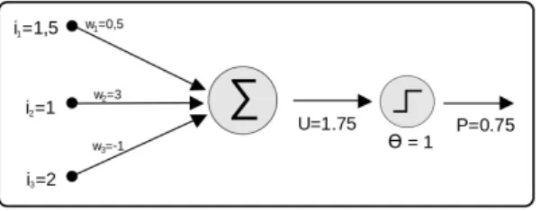
Taking inspiration from biology, in 1943 McCulloch and Pitts introduced the notion of artificial neuron, which is shown in figure 1.3.
Figure 1.3: Artificial Neuron
An artificial neuron is essentially a function that takes input from other neurons. Each input is associated to a weight. Inside the neuron, which is represented as a circle in the figure above, the dot product (input x weights) is calculated and then an activation function is applied.
The activation function is typically the Standard Logistic Function, or any function that belongs to the Sigmoid family:
f(x) =
1 1 + e xi
Where xi is the dot product given a neuron at index i:
xi=
X
wi⇥ pi
Properties of the Standard Logistic Function: • Dom: [-1,1], Cod: [1,0]
• limx! 1f (x) = 0, limx!1f (x) = 1
Another common activation function is the Hyperbolic Tangent, shown in figure 1.5:
Figure 1.5: Hyperbolic Tangent
f (x) = tanh(x) Properties of the Hyperbolic Tangent: • Dom: [-1,1], Cod: [-1,+1]
• limx! 1f (x) = 1, limx!1f (x) = 1
Sigmoid functions are often used in Neural Networks (ANN) to introduce non-linearity into the model and to ensure that certain signals remain within
specific ranges. A popular artificial neural element computes the linear com-bination of the corresponding input signals and applies a sigmoid function limited to the result. This model can be seen as a ”regular” variant of the classical threshold neuron.
1.3.2
Artificial Neural Network
An Artificial Neural Network (ANN) is obtained by grouping di↵erent artificial neurons into di↵erent layers. Figure 1.6 shows an example of ANN.
Figure 1.6: Artificial Neural Network
An Artificial Neural Network (ANN) is composed of a series of neurons, represented as circles in the figure, which take as input the weights of the edges coming from the neurons of the previous level. The ANN then calcu-lates the dot product and applies the activation function to the result and it propagates the output to the next level. A network with these charac-teristics is called feedforward because the output always goes towards the next layer. Another feature of the network shown in the figure is that of being fully connected : each neuron propagates the result of its computation to each neuron of the following layer. A network that is both feed-forward and fully connected is called Multilayer Perceptron (MLP). A neural network is considered ”deep” when several layers are stacked and each layer contains thousands of neurons. Recent models present between 7 and 50 layers.
The core of the Deep Learning algorithms consists in finding the right weights at the edges of the network so that the sum of the errors of the output neurons is minimized. To achieve this goal it is necessary to establish:
• which function to use in each neuron (activation function).
• which function to use to calculate the sum of errors (loss function). • which algorithm to use to find the right weights of the network
(back-propagation algorithm).
We have already explained the meaning of the activation function, thus no further clarification is needed. Concerning the loss function, one of the most used, especially for regression problems, is the Mean Square Error (MSE):
⌘(w, x) = 1 n
X
tc zc2
Where:
• z represents the output vector produced by the network z = [z1, .., zn]
• x represents the input vector x = [x1, .., xn]
• t represents the desired output.
The aim of the Deep Learning algorithms is to find parameters (weights) and hyper-parameters to minimize the total MSE. The most used method is the backpropagation algorithm, which consists in tracing back the network (from the output level up to the input level) and adjusting the weights, which in principle are initialized randomly. At each step, the new weights are calculated using the gradient descent, a well known optimization technique that allows to find local minimum of multi-variable functions, and therefore to minimize the error, according to an additional parameter called Learning Rate. This latter parameter determines the speed of convergence of the gradient: if the learning rate is too high, the algorithm converges quickly but risks overshooting, e.g.: not finding the local minimum and continuing to
oscillate among more possible solutions. Viceversa, if the learning rate is too small, the gradient descent algorithm risks converging too slowly. Learning is therefore a complex optimization problem because the number of weights involved can be very high. Recent models reach up millions of parameters.
1.3.3
Convolutional Neural Network
Artificial Neural Networks, in particular the MLP model, are extremely powerful because, according to the Universal Approximation Theorem, are capable of approximating any function. However, they do not apply well to images. In fact, images are 2D grid structured arrays. Given a few mil-lion pixels, the parameters explode. In addition, images have transversely repeated patterns. It is possible to exploit the presence of patterns to give the same weights to the edges and make the problem easier for computers. The same thing happens in the brain: data coming through the retina to the primary visual cortex (v1) pass through neural layers that create hierarchical features. This process is illustrated in figure 1.7.
Figure 1.7: Visual Cortex System
The intuition stems from an experiment by D.Wiesel and T. Hubel [4], which dates back to 1962, when the two researchers realized that cats, and similarly humans, have two types of cells: simple and complex cells. Simple cells are excited to recognize small and simple patterns, while complex cells aggregate information from simple cells to recognize more generic patterns.
There is a hierarchy of simple and complex cells which is repeated. This repetition creates a hierarchical structure, where initial the layers are able to recognize simple patterns, while complex patterns are distinguished by the last layers.
Convolutional neural networks (CNN) are based exactly on the same hierar-chical representation. However, instead of using a fully connected network, a local filter convolution is applied to every area of the input image. The con-volution operation is essentially a filter that is passed over every area of the input image of the CNN. This operation, described in figure 1.8, represents exactly the simple cell.
Figure 1.8: Convolution operation with filter
The complex cell is instead represented by the pooling operation: it takes a set of simple cells and applies an operation that is typically the maximum or the average to aggregate information. The idea is to present a sort of ’summary’ to the next level, so we use the maximum or the average. Pooling operation is shown in figure 1.9.
CNNs apply a convolution layer and a pooling layer in series. At the end there is always a fully connected layer, that is the classifier, and it classi-fies the learned features. The result is a neural network where weights are shared and connections to the next level are local. As a consequence, the number of weights to be found is much lower than an MLP, so the problem, computationally speaking, is easier. The activation function typically used
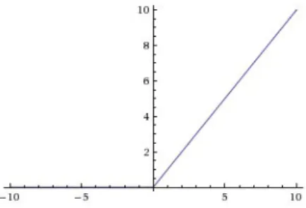
Figure 1.9: Pooling operation using max, 2x2 filter and stride=2 in CNNs is the ReLU (figure 1.10), which is similar to a sigmoid, but has some advantages that favors convergence:
Figure 1.10: ReLU, Rectified Linear Unit
f (x) = max(0, x)
The ReLU as activation function implies that neurons are activated in a sparse manner. Combining convolution and pooling, CNNs are excellent for image classification problems. Hence, the final architecture for Convolutional Neural Network is shown in figure 1.11:
Figure 1.11: Convolutional Neural Network
1.4
Training details
During the training phase, hyper-parameters are particularly relevant. This section aims at analyzing the most important parameters, the one that can a↵ect the training phase the most in terms of training time, convergence and accuracy.
1.4.1
Stochastic Gradient Discent
Stochastic Gradient Descent (SGD) is one of the most popular optimiza-tion algorithms. It is widely used in neural networks as it is the basis of the backpropagation algorithm. The idea of the SGD is to minimize an objective function J(x) formed by N parameters by updating the value of the parameters based on the di↵erence with the negative gradient of J(x). The parameter is then updated step by step, according to a given value LR, called the Learning Rate. In short, we descend a function J(x) step by step, until this leads us to a local minimum value. How long is the step? This corresponds to the Learning Rate value, as shown in figure 1.12.
Figure 1.12: SGD and Learning Rate
1.4.2
SoftMax as function for the output level
As already explained, it is possible to use both tan(h) or the Standard Logistic Function as activation functions on the output layer . In the first case, output values are included between -1 and 1. Using a Standard Logistic Function, output values will be included between 0 and 1. However, in both cases there is no guarantee that the sum on the output neurons is 1, which is a fundamental requirement so that they can be interpreted as a probabilistic distribution.
When a neural network is used as a multi-class classifier, the use of the Soft-Max activation function makes it possible to transform the values produced by the last level of the network into class probabilities:
sof tmax(x) = e
x
P
1..nex
1.4.3
Cross-Entropy as loss function
Using MSE as a loss function is not an optimal choice for classification since the output values do not represent probabilities and the non-imposition of the sum constraint equal to 1 makes learning less e↵ective [5]. Given a multiclass classification problem, the use of Cross-Entropy as a loss function is highly recommended:
CE(x) = Xp(x)⇥ log(q(x))
Cross-entropy is mostly used to understand the di↵erence between two probability distributions. The target distribution, the one that the model is trying to match, is expressed in terms of a one-hot distribution. How close is the predicted distribution to the real distribution? That is what the cross-entropy loss determines. In the formula above, p(x) stands for the target probability, while q(x) represents the actual probability.
1.4.4
Regularization
Regularization techniques can be used to reduce the risk of overfitting by a neural network with many parameters. This trick is very important when the training set is not large compared to the capacity of the model. Neural networks whose weights are close to zero tend to be more stable and this often leads to a better generalization [5]. To force the network to adopt weights of small value, a regularization term to the loss can be added. For instance, in the case of Cross-Entropy Loss:
Jtot = CE + Jreg
Jreg can be obtained as follows:
• L1: Jreg= P|wi|
• L2: Jreg= 12 ⇥ Pwi2
In both cases the parameter can be set arbitrarily. L1 can have a sparsifying e↵ect (i.e. bring numerous weights to 0) greater than L2. In fact, when the weights assume values close to zero, the calculation of the square in L2 has the e↵ect of excessively reducing the corrections to the weights, making it difficult to reset them.
1.4.5
Momentum
While stochastic gradient descent remains a popular optimization strat-egy, learning with it can sometimes be slow. The method of momentum is designed to accelerate learning, especially in presence of high curvature, small but consistent gradients, or noisy gradients [6]. The momentum algorithm accumulates an exponentially decaying moving average of past gradients and continues to move in their direction. The name momentum derives from an analogy with physics, in which the negative gradient is a force moving a particle through parameter space, according to Newton’s laws of motion. Momentum in physics is mass times velocity. In figure 1.13 it is possible to see the e↵ect of the momentum, draw in red lines.
Figure 1.13: The e↵ect of momentum
1.4.6
Learning Rate
We said before that learning rate is an hyper parameter that represents how long is the step while moving towards a local minimum. This definition implicitly means that steps must be of the same length. In this scenario, we would probably choose a short step, meaning a low value for the LR, because
we want to be sure to find a local minimum and to avoid overshooting, despite the fact that this would be time consuming. However, it is easy to understand that the best choice would be that of taking a ”longer” step when we are far from the minimum, and of progressively decreasing the length of the step as we get closer to the solution. This can be achieved by using predefined learning rate schedules or adaptive learning rate methods.
Learning Rate Schedules
Learning rate schedules aim at adapting the learning rate during training by planning a predefined schedule. Learning rate schedules methods are: time-based decay, step decay and exponential decay.
Time-Based Decay can be expressed in mathematical form as follows: lr = lr0/(1 + kt)
where lr, k are hyperparameters and t is the iteration number. The learning rate is updated by a decreasing factor in each epoch.
Step Decay schedule drops the learning rate by a factor every few epochs. The mathematical form of step decay is :
lr = lr0⇥ dropf loor(
epoch epochsdrop)
A typical way is to to drop the learning rate by half every 10 epochs. Another common schedule is exponential decay:
lr = lr0 ⇥ e kt
where lr, k are hyper parameters and t is the iteration number. Adaptive Learning Rate
There is still one issue to be discussed concerning the use of the learning rate schedule: hyper-parameters must be defined a priori and the same hyper parameters are applied for each update. Sometimes, we may be interested
in updating the parameters in di↵erent extent. A better way to do this is to use Adaptive gradient descent algorithms: Adadelta, Adagrad, Adam, RMSprop. These methods use a heuristic approach, avoiding extensive fine tuning for the hyper-parameters.
Adagrad adapts the learning rate performing updates: frequently occur-ring features are associated with smaller updates, while infrequent features are associated with larger updates. Due to this behaviour, Adagrad is well-suited for dealing with sparse data. Previously, an update over all parameters ⇥ was performed using the same learning rate ⌘. Adagrad uses a di↵erent learning rate for every parameter ⇥i at every time step t.
Adadelta is an extension of Adagrad that seeks to reduce its aggressive, monotonically decreasing learning rate. Instead of accumulating all past squared gradients, Adadelta restricts the window of accumulated past gradi-ents to some fixed size [7].
Adam (Adaptive Moment Estimation) calculates adaptive learning rates for each parameter. In addition to storing an exponentially decaying average of past squared gradients, Adam also keeps an exponentially decaying average of past gradients, similar to momentum [8].
There are still other methods as adaptive learning rate that are not men-tioned. At this point, one might be wondering which criteria we must con-sider for picking up the right learning rate method. The truth is that, despite Adam being considered the state of the art, there is no rule for this task. In fact, training a neural network requires experience, and hyper-parameters tuning depends on the problem, the architecture of the network, the dataset, the domain and other details. Experience in training neural architectures surely plays a key role [9].
Computer Vision
T.S. Huang provides a brilliant definition for Computer Vision [10]. Com-puter Vision has a dual goal. From the biological science point of view, com-puter vision aims at providing computational models of the human visual system. From an engineering point of view, computer vision aims at build-ing autonomous systems which could perform some of the tasks which can also be performed by the human visual system (and even surpass it in many cases). Of course, the two goals are intimately related. The properties and characteristics of the human visual system often give inspiration to engineers who are designing computer vision systems. Conversely, computer vision al-gorithms can o↵er insights into how the human visual system works.
The tasks of Computer Vision typically are:
• Image Classification: it is the task of assigning a label, from a fixed set of categories, to an input image. This is one of the core problems in Computer Vision that, despite its simplicity, presents a large variety of practical applications.
• Image Classification and Localization: given an image, what we want is the most relevant object and provide a rectangle to identify where the object is.
• Object Detection: given an image, the aim of object detection is to 19
extract relevant objects and their location. This means that object detection is not just a classification task, but also a regression task. In fact, the final output is a label plus a tuple of numbers: x0, y0, width,
height.
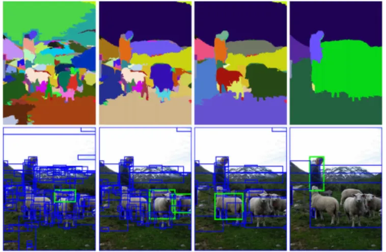
• Instance Segmentation: it can be considered as a sort of object recogni-tion, with the di↵erence that in this case segmentation is more precise, because it creates an area that overlaps the detected object. The result of image segmentation is a set of segments that collectively cover the entire image, or a set of contours extracted from the image [11].
Figure 2.1: Image Classification, Localization, Detection and Segmentation
All these tasks are illustrated in figure 2.1. In this thesis, we will focus mainly on Object Detection.
2.1
Deep Architectures for Object Detection
This section will introduce the main architectures that exploit Deep Learn-ing for Object Detection. It should be noted that the architectures proposed are the result of a fairly recent scientific work which is in constant evolution. All these models share the same core: they are all based on Convolutional Neural Networks (CNN).
2.1.1
R-CNN
The purpose of the R-CNN (Region CNN) [12] is to identify the main objects given an input image. Therefore, the first step is identifying the re-gions where the objects could potentially be and subsequently applying CNNs for the identification phase. This phase, called Regions Proposal Phase, is computed through an algorithm called Selective Search [13]. This algorithm considers the image through windows of di↵erent sizes, and for each dimen-sion tries to group adjacent pixels by texture, color or intensity, as shown in figure 2.2.
Figure 2.2: Selective Search
The result of this phase are the Regions of Interest, which are areas of the starting image that contain potential objects to be detected. Each Region of Interest is adjusted to ensure that the input of the Region of Interest matches the CNN (warping phase). Each image is processed by CNN, typically AlexNet, and then SVM is applied for the classification task, on the last layer, the fully connected one, while Bounding Box Regression is used for the localization task. The initial regions proposed by the Selective Search algorithm may not be perfectly centered with respect to the subject they contain. Precisely for this reason, the last step of Bounding Box Regression is a further refinement to ensure that the subject is centered in relation to
the coordinates of the rectangle in which it is inscribed. Therefore we can consider the R-CNNs just like CNN, where the input is suggested by the Selective Search algorithm and the last layer performs the classification task using SVM. It is evident that the R-CNNs su↵er from a critical problem: each Region of Interest becomes the input of a CNN, so the number of CNNs is equal to the number of Regions of Interest, usually a few thousands per image. This makes the problem not suitable for real-time applications, where the detection time must be almost instantaneous. Figure 2.3 shows R-CNN architecture.
Figure 2.3: R-CNN
2.1.2
Fast R-CNN
Fast R-CNNs [14] are a further improvement of the R-CNN. The substan-tial di↵erence consists in placing a RoI Pooling layer between the CNNs and the last fully connected level. While with the R-CNN the components to be trained were CNN, SVM and Bounding Box respectively, the Fast R-CNNs are better because only one component (the RoI Pooling layer) is used for the training phase. The RoI Pooling layer receives as input both the Region Proposals, obtained again by the Selective Search algorithm, and the last layer of CNN. The resulting output are vectors that have the same size that are processed by the fully connected layer. Similarly to the classical R-CNNs,
classification and regression are made on the basis of this last level, with the di↵erence that the classification task is no longer assigned to SVM but to the Soft-Max algorithm, which returns a confidence value. The regression part remains unchanged, using the Bounding Box Regressor. Figure 2.4 shows the Fast R-CNN architecture, while figure 2.5 shows just the RoI Pooling Layer.
Figure 2.4: Fast R-CNN Architecture
Figure 2.5: RoI Pooling Layer
When analyzing the architecture of a Fast R-CNN network, it is clear that all the inputs and outputs necessary for the classification and localization tasks come from a single network, which therefore proves to be much more efficient than a classic R-CNN, where to each object there corresponds a CNN.
2.1.3
Faster R-CNN
Even with all these improvements, a sore point remains in the (Fast) R-CNN: the Region Proposal phase. As we have seen, the first step to discover the position of objects is to generate a lot of potential regions of interest to be tested. The Selective Search algorithm is quite slow and turns out to be the bottleneck of the whole process. The Faster R-CNNs [8] distinguish themselves precisely because they are able to make classification and region proposals thanks to a single CNN. In fact, note that the RoIs strongly depend on the features extracted from the image, which are also calculated by the first levels of CNN. Why not using the same results coming from the CNN for region proposals instead of running the Selective Search separately? This way we obtain the regions of interest almost for free, the only shrewdness is to train the CNN.
Faster R-CNNs consist of two modules:
• RPN (Region Proposal Network): given the input of the convolutional layer, it finds the rectangles for the localization. These rectangles are identified only if there is a relevant subject inside.
• RoI Pooling Layer: classifies each proposal and applies a correction factor so that the subject is centered with respect to the rectangle in which it is inscribed.
The Region Proposal Network (RPN) is definitely the element that makes Faster R-CNN more interesting than the approaches seen so far. Specifically, the RPN uses a sliding window that is scrolled on the feature map and classifies what is below the sliding window as an object/non-object proposing a bounding box in the first case. However, we know that these bounding boxes will have di↵erent proportions depending on the object that has been identified. For example, a person will be framed in a rectangle where the height will be significantly greater than the width. Vice versa, a TV monitor will be identified by a rectangle with a 4: 3 aspect ratio. The RPN also deals with finding rectangles with the appropriate proportions. To do so, we
propose a series of anchor boxes with associated confidence values. Anchor boxes whose confidence value falls below a certain threshold are discarded, while the rest are passed to the RoI Pooling layer for the classification phase. Figures 2.6 and 2.7 show respectively the Faster R-CNN architecture and the RPN.
Figure 2.6: Faster R-CNN Architecture
2.1.4
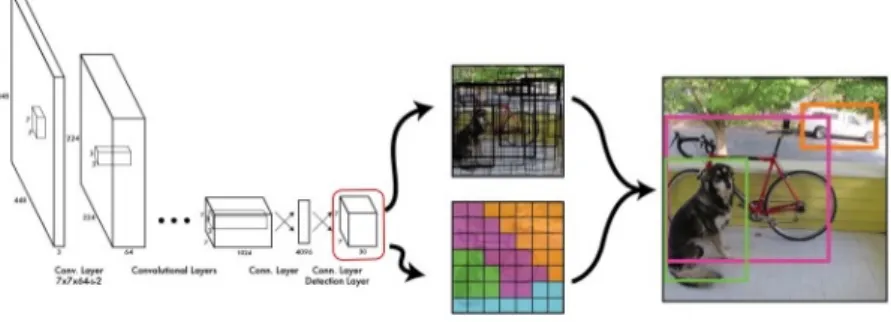
YOLO
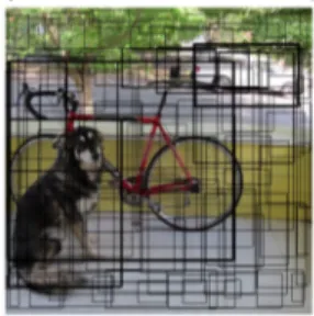
Previous detection systems reuse classifiers or locators to perform detec-tion. They apply the model to an image in multiple positions and scales. Regions with a high image score are considered relevant. YOLO [15] uses a completely di↵erent approach. A single neural network is applied to the entire image. In fact, YOLO stands for You Only Look Once. This network di-vides the image into regions and calculates bounding boxes and probabilities for each of them. This approach has several advantages over classifier-based systems. It makes predictions with a single evaluation of the network, unlike systems like R-CNN that require thousands of evaluations for a single image. How is it possible to do everything with a single neural network? The first step of the processing is to divide the input image into a grid, where each cell is responsible for predicting bounding boxes and their respective confidence values. If the box contains an object, the associated confidence value will be very high, vice versa if it does not contain any object, then the confidence will be very low. This step is shown in figure 2.8.
Figure 2.8: YOLO, image divided into bounding boxes
At this point we know exactly how many relevant objects there are in the image, but not what they are. Therefore, each cell also takes care of calculating the probability that for the object to belong to a certain class (class probability), as shown in figure 2.9.
We are talking about conditional probability, which means that the cal-culated value does not represent the probability to contain that object; it means that if that cell contains an object, then the probability for that
ob-Figure 2.9: YOLO, class probabilities
ject to be a bike, a dog or a car is equal to the calculated value. Subsequently the class probability is multiplied by the conditional probability to obtain a grid where each bounding box considers both the probability of containing this object related to the possibility that there is an object inside. Figure 2.10 illustrates this process.
Figure 2.10: YOLO, bounding box and conditional
We then consider only the rectangles whose confidence value is higher than a certain threshold, which is described in figure 2.11.
Despite some generalization errors, YOLO represents the state of the art in object detection algorithms and its speed in detecting objects inside images makes the network particularly adaptable to solve tasks in real time. The architecture of YOLO is summarized in figure 2.12.
The same authors of YOLO have then introduces some improvements in order to enhance the processing time such as anchor boxes generation and a
Figure 2.11: YOLO, threshold detection
Figure 2.12: YOLO architecture
tree data structure allowing the label sharing between detection and classi-fication, since detection usually has coarse grained label, which corrisponds to the parent node in the tree [16] [17].
2.1.5
SSD Multibox
In November 2016, Wei Liu et al.[18] introduced the Single Shot Multi-Box Detector. SSD speeds up the processing phase by eliminating the RPN. Starting from a small convolution filters, SSD is able to calculate both lo-cation and class score. Then, feature maps are extracted and a convolution filter is applied to each cell. What is new is the multi-scale feature maps: multiple layers are used to detect objects independently. This is done by 6 convolution layers after the VGG-16 layer [19]. In fact, VGG-16 as base
net-work is a brilliant idea due to its strong performances in image classification and its popularity for problems where transfer learning helps in improving results. Thus, a set of convolution layers enables multiple scale feature ex-tractions while decreasing the size of the input layer step by step.
Figure 2.13: SSD architecture
In addition, extra convolutional layers help handling bigger objects, while the non-maxima suppression algorithm is used to filter multiple boxes that may appear. The final architecture is exposed in figure 2.13. The model is quite simple if compared to previous architecture because it discards the proposal generation step. All the processing phase is handled in a single network. Despite SSD could seem similar to YOLO, it is necessary to remark that YOLO uses predefined grid cells, so the aspect ratio is fixed, while SSD allows more aspect ratios (6 in total). Due to this reason, SSD bounding boxes are generally more accurate than the one predicted by YOLO.
2.1.6
Performance evaluation
mAP stands for mean Average Precision and it is considered the standard measure for evaluating object detection algorithms by the scientific commu-nity. Here we should remember that that object detection means both clas-sification and regression, we need a measure for evaluating both tasks at the same time. Using accuracy as metric would introduce some biases. In fact, a typical data set may contain many classes and their distribution is non-uniform (for example, there might be many more cats than cars). To face this problem, we must introduce the notion of Precision and Recall:
P recision = true object detections
total number of detections by the system
A precision value close to 1 means that whatever the classifier predicts as positive is in fact a correct prediction.
• Recall measures the false negative rate:
Recall = true object detections
total number of objects in the data set
A recall value close to 1 means that almost all objects in the dataset will be positively detected.
Precision and Recall are linked by a relationship of inverse proportionality: when one grows, the other decreases and vice versa. For instance, if we want to calculate the AP (Average Precision) for the class ’dog’, the Preci-sion/Recall curve is created by varying the threshold that determines what is considered as a model-predicted positive detection of the class, as shown in figure 2.14.
Figure 2.14: Precision-Recall curve for the class dog Given this curve, AP can be calculate as follows:
AP = 1 n
X
Recalli
P recision(Recalli)
Concerning the localization problem, the most common metric is the In-tersection over the Union (IoU). The basic idea is to provide a number scoring how well the ground truth object overlaps the object boundary predicted by
the model. IoU can even be explained visually, which makes everything easier to understand. Figures 2.15 and 2.16 explain IoU visually.
Figure 2.15: Intersection over the Union
Again, the IoU threshold is a fundamental parameter and, as previously stated, we can calculate Precision-Recall by varying IoU thresholds.
Figure 2.17: Precision/Recall curve for IoU
In figure 2.17 dashes represent spaced recall values where the AP is cal-culated. Finally, the mean Average Precision or mAP score is equal to the mean AP over all classes and over all IoU thresholds. This way there is only one score that comprehends both classification and localization. However, thresholds may vary depending on the competition or dataset. Right now, we can evaluate all the deep learning architectures for object detection that have been previously explained. Table 2.1 compares di↵erent deep architec-tures for object detection [20].
mAP Speed (FPS) Speed (s/img)
R-CNN 62.4 .05 FPS 20 s/img
Fast R-CNN 70 .5 FPS 2 s/img
Faster R-CNN 78.8 7 FPS 140 ms/img
YOLO 63.7 45 FPS 22 ms/img
SSD 74.3 59 FPS 29 ms/img
Table 2.1: Object Detection performances, tested on Pascal VOC
It is necessary to specify that the table below has been elaborated to give a summary view of the main characteristics of these networks. To be more precise, each of these neural networks should be evaluated in their versions
and updates. In addition, although Pascal VOC is considered the standard by the scientific community, there are also other datasets on which to perform benchmarking such as COCO, ImageNet etc. However, data show that:
• R-CNNs are the worst solution both for accuracy and speed.
• R-CNNs, Fast R-CNNs, Faster R-CNNs clearly show a huge bottleneck due to the selective search algorithm.
• YOLO and SSD are nearly the only two suitable for solving real-time tasks.
In the next chapters we will first introduce Tensorflow for Object Detec-tion and we will then focus on those networks that can solve real-time tasks and, at the same, optimize the use of resources (computing, memory, battery capacity), a typical scenario of embedded systems.
Tensorflow for Object
Detection
Tensorflow is the most popular library for Machine Learning. It was ini-tially built for scaling and running over multiple CPUs and now it is even available for mobile operating systems. In Tensorflow models are represented as a dataflow graph that contains a set of nodes described as operations. These are units of computation: they can be simple, as addition or multi-plication, but also complicated, such as convolutions. Each operation takes as input a tensor and it provides a new tensor as output. Tensors are just the way data are represented in Tensorflow, they are multidimensional ar-rays of numbers and they flow among operations. This chapter provides basic notions for building Machine Learning models using Tensorflow, introducing:
• High Level APIs (Keras and Eager Execution) • Low Level APIs (Tensors, Graphs and Sessions)
The content of this chapter is a small summary of Tensorflow documenta-tion. The aim is to provide a general overview of the concepts that underlie the construction of deep learning models [21].
3.1
High Level APIs with Keras
Keras is a high-level API to design deep learning models. It is used for fast prototyping, advanced research and production, with three key advantages:
• User friendly: a simple interface optimized for common use cases. It provides a clear feedback regarding user errors.
• Composable: Keras models are made by connecting configurable build-ing blocks together.
• Easy to extend: writing custom layers, creating new layers, loss func-tions.
What developers do with Keras is, essentially, composing layers for building models. The basic model is the sequential: tf.keras.Sequential. This is a simple Multilayer Percepetron model:
import tensorflow as tf
from tensorflow import keras model = keras.Sequential()
model.add(keras.layers.Dense(64, activation=’relu’)) model.add(keras.layers.Dense(64, activation=’relu’)) model.add(keras.layers.Dense(10, activation=’softmax’))
The above mentioned code creates a MLP with 3 layers: 64 neurons for layers 1 and 2 with ReLU as activation function, while the last layer has 10 output neurons using softmax for classification.
We can train and evaluate this model using the ’compile’ method with 3 arguments:
• Optimizer: This object specifies the training procedure. We can spec-ify which kind of training policy to adapt, such as AdamOptimizer, RMSPropOptimizer, or GradientDescentOptimizer.
• Loss: The function used to calculate the error during the optimization phase. Common choices include mean square error (MSE) or Cross Entropy.
• Metrics: Used to monitor training. These are string names or callables from the tf.keras.metrics module.
By calling the ’compile’ method we can train and evaluate the model:
model.compile(optimizer=tf.train.AdamOptimizer(0.001), loss=’categorical_crossentropy’,
metrics=[’accuracy’])
Before starting the training phase, we need to set up the dataset. This can be easily done by in-memory Numpy Arrays and using the ’fit’ method, that takes 3 arguments: epochs, batch size and validation data.
import numpy as np
data = np.random.random((1000, 32)) labels = np.random.random((1000, 10))
model.fit(data, labels, epochs=10, batch_size=32)
In case we need bigger datasets or we just need to clean data before process-ing them, Keras APIs provide all the methods to perform these operations. Lastly, we can evaluate the model and predict new data:
model.evaluate(x, y, batch_size=32) model.evaluate(dataset, steps=30) model.predict(x, batch_size=32) model.predict(dataset, steps=30)
The final code for a simple fully connected neural network (MLP) is:
inputs = keras.Input(shape=(32,))
x = keras.layers.Dense(64, activation=’relu’)(inputs) x = keras.layers.Dense(64, activation=’relu’)(x)
model = keras.Model(inputs=inputs, outputs=predictions) model.compile(optimizer=tf.train.RMSPropOptimizer(0.001),
loss=’categorical_crossentropy’,metrics=[’accuracy’]) model.fit(data, labels, batch_size=32, epochs=5)
For instance, it is extremely easy to build a MNIST classifier [22] using Keras:
import tensorflow as tf
# downloading the mnist dataset
mnist = tf.keras.datasets.mnist
# splitting test and train set
(x_train, y_train),(x_test, y_test) = mnist.load_data() x_train, x_test = x_train / 255.0, x_test / 255.0
# composing the model
model = tf.keras.models.Sequential([ tf.keras.layers.Flatten(), tf.keras.layers.Dense(512, activation=tf.nn.relu), tf.keras.layers.Dropout(0.2), tf.keras.layers.Dense(10, activation=tf.nn.softmax) ])
# configuring the training parameters
model.compile(optimizer=’adam’,
loss=’sparse_categorical_crossentropy’, metrics=[’accuracy’])
# start the training
model.fit(x_train, y_train, epochs=5)
# evaluating the model
model.evaluate(x_test, y_test)
3.2
High Level APIs with Eager Execution
What makes Tensorflow eager execution di↵erent from Keras APIs is the fact that operations are evaluated immediately, with no graph needed. In fact, operations return values without building the entire graph. It can be a good choice for getting started with Tensorflow and for debugging the model. The main advantages are:
• An intuitive interface: structure your code using Python data struc-tures. Quickly iterate on small models and small data.
• Easier debugging: call operations directly to inspect models.
• Natural control flow: use procedural control flow instead of Tensorflow graph.
By enabling tf.enable eager execution() TensorFlow operations will re-turn the result immediately:
import tensorflow as tf tf.enable_eager_execution() x = [[2.]]
m = tf.matmul(x, x)
print(m) #[[4.]]
Since there is not a computational graph to build and run later in a session, it is easy to inspect results using ’print()’ or a debugger. Evaluating, printing, and checking tensor values does not break the flow for computing gradients [21].
Models can be organized in classes. Here is a model class that creates a two layer neural network that can classify the standard MNIST handwritten digits.
class MNISTModel(tfe.Network):
def __init__(self):
super(MNISTModel, self).__init__()
self.layer1 = self.track_layer(tf.layers.Dense(units=10)) self.layer2 = self.track_layer(tf.layers.Dense(units=10))
def call(self, input):
# Actually runs the model
result = self.layer1(input) result = self.layer2(result)
The ’build’ method is called the first time the layer is used. It is possible to create variables during init () if their full shapes are already known. We use tfe.Network, which is a container for layers. It also contains utilities for inspection, saving and restoring values. Even without training the model, we can imperatively call it and inspect the output:
model = MNISTModel()
batch = tf.zeros([1, 1, 784])
print(batch.shape) # (1, 1, 784)
result = model(batch)
print(result)
# tf.Tensor([[[0., ..., 0]]], shape=(1, 1, 10), dtype=float32)
To train any model, we define a loss function to optimize, calculate gradients, and use an optimizer to update the variables.
def loss_function(model, x, y): y_ = model(x) return tf.nn.softmax_cross_entropy_with_logits(labels=y, logits=y_) optimizer = tf.train.GradientDescentOptimizer(learning_rate=0.001) for (x, y) in tfe.Iterator(dataset): grads = tfe.implicit_gradients(loss_function)(model, x, y) optimizer.apply_gradients(grads)
3.3
Low Level APIs: Tensors, Graphs and
Sessions
If you really want to know how Tensorflow works at its cor,e then Low Level APIs are needed, which consist of three elements:
• Tensors • Graphs
• Sessions
The central unit of data in Tensorflow is the tensor. A tensor consists of a set of primitive values shaped into an array of any number of dimensions. Given a tensor, its rank is the number of dimension, and its shape is a tuple of numbers specifying the array lenght for each dimension. Tensorflow uses numpy arrays to represent tensor values. [23]
A computational graph is a series of operations. The graph is composed of two types of objects:
• Operations: these are the nodes of the graph. The input is a tensor and the output is another tensor.
• Tensors: these are the edges in the graph. They are the values that flow through the graph.
A simple computational graph for adding two numbers can be coded as fol-lows:
a = tf.constant(3.0) b = tf.constant(4.0) total = a + b
print(total) #this will not print 7.0
Printing the value of the tensor will not provide the final result. To execute this graph you need to start a session. A session encapsulates the state of the Tensorflow runtime, and runs Tensorflow operations. A tf.Session object is like the python executable:
sess = tf.Session()
print(sess.run(total)) # 7.0
A graph can be parameterized to accept external inputs, known as place-holders. A placeholder is a promise to provide a value later, like a function argument.
y = tf.placeholder(tf.float32) z = x + y
We can use Placeholders for simple experiments, but Datasets are the pre-ferred method of streaming data into a model. To get a runnable tf.Tensor from a Dataset you must first convert it to a tf.data.Iterator, and then call the Iterator’s get next method. Creating an iterator is easy with the make one shot iterator method. For instance, in the code below the next item tensor will return a row from the my data array on each run call:
my_data = [ [0, 1,], [2, 3,], [4, 5,], [6, 7,], ] slices = tf.data.Dataset.from_tensor_slices(my_data) next_item = slices.make_one_shot_iterator().get_next()
We will now see how to built a feedfoward neural network using Low Level APIs: # Define placeholders X = tf.placeholder(tf.float32, shape=[None, 4]) y = tf.placeholder(tf.int32, shape=[None, 3]) # Define variables w1 = weight_variable([1], 2]) b1 = bias_variable([2]) w2 = weight_variable([2, 3]) b2 = bias_variable([3]) # Define network # Hidden layer z1 = tf.add(tf.matmul(X, w1), b1) a1 = tf.nn.relu(z1) # Output layer
z2 = tf.add(tf.matmul(a1, w2), b2) y_pred = tf.nn.softmax(z2)
y_one_hot = tf.one_hot(y, 3)
# Define loss function
loss = tf.losses.softmax_cross_entropy(y, y_pred, reduction=tf.losses.Reduction.MEAN)
# Define optimizer
optimizer = tf.train.AdamOptimizer(0.01).minimize(loss)
# Metric
accuracy = tf.reduce_mean(tf.cast(tf.equal(tf.argmax(y, axis=1), tf.argmax(y_pred, axis=1)), tf.float32))
for _ in range(n_epochs):
sess.run(optimizer, feed_dict={X: X_train, y: y_train})
In this example, variables X train and y train contain the whole training set, mini-batches as big as the whole dataset. It is clear that building a MNIST classifier using Low Level API is quite complex. We will not focus on this part, but if you are interested the code is available on Github: https://github.com/cjalmeida/tensorflow-mnist
3.4
Tensorflow Object Detection APIs
Designing accurate machine learning models capable of localizing and identifying objects in a single image remains a core challenge in computer vision. The TensorFlow Object Detection API is an open source framework built on top of TensorFlow that makes it easy to construct, train and deploy object detection models. Object Detection is based on low level APIs and has nothing to do with Keras or Eager Execution. This section will provide a general overview about how object detection APIs work, more details will be given in chapter 4.
3.4.1
Training a model and export a frozen graph
Object Detection APIs are a set of classes for training custom models for object detection. The good point is that the general architecture does not require to code writing for the training phase. In fact, the training is completely handled by a config file, where the developer can specify:
• Model configuration: this defines what type of model will be trained. • Train configuration: decides what parameters should be used during
the training.
• Evaluation configuration: determines what set of metrics will be re-ported for evaluation.
• Training input: defines what dataset the model should be trained on. • Evaluation input: defines what dataset the model will be evaluated on. Once all these things are defined, we still need a file for the labels and .record files that contain the images for the training and evaluation phases in a Tensorflow own binary storage format. Labels can be expressed in a .pbtxt file according to the following pattern:
item { id: 1 name: ’class_name_1’ } item { id: n name: ’class_name_n’ }
TF record files can be created by simply using using the generate tfrecord.py class that is included in the Object Detection package. This class needs a .csv as input and it provides a .record file as ouput. After that, it is easy to setup a training pipeline. The library has already some examples available, which may be customized just by changing some parameters. The training phase can be started by running:
python legacy/train.py --logtostderr
--train_dir=train_directory
--pipeline_config_path=CONFIG_FILE
Concurrently, we can run the evaluation phase:
python legacy/eval.py --logtostderr
--pipeline_config_path=CONFIG_FILE
--checkpoint_dir=directory_to_save_checkpoints --eval_dir=eval_directory
The training phase continuously generates checkpoints, which contain the weights of the network, that are evaluated by eval.py. Through Tensorboard it is possible to monitor the whole process. Tensorboard can be started by typing: