POLITECNICO DI MILANO
SCUOLA DI INGEGNERIA INDUSTRIALE E DELL’INFORMAZIONE
Master of Science in Automation and Control Engineering
A comparison among different
sampling-based planning techniques
Name: Carlos Martínez Alandes Matriculation number: 820937 Supervisor: Prof. Luca Bascetta Co-supervisor: Eng. Matteo Ragaglia
Acknowledgements
I want to acknowledge my family because nothing would have been possible without their support, not just economical but also moral and psychological, for bringing me this incredible chance to become better student and better person.
I would like to acknowledge also my tutors, who have been helping and being patience with me every moment during this thesis.
Abstract
Nowadays the applications of the robotics are becoming infinite. We can find robots in every aspect of the life, even if we often don’t realize that we are in front of one. We can differentiate some kinds of robots: some of those robots are controlled by an operator, other are set to do some specific job/movement, and others work autonomously with total independence on the operator, interacting by themselves with the environment. In this thesis we are focusing on this last kind of them, and we are going to introduce one of the most widely used libraries in terms of path planning, the OMPL (Open Motion Planning Library) and elab-orate a comparison among all the sampling based planning methods included in this library. To do so, we will create an specific problem that will be solve by different methods.
Oggi le applicazioni dei robot stanno diventando infinite. Possiamo trovare i robot in ogni aspetto della vita, anche se spesso non ci rendiamo conto che siamo di fronte ad uno. Possiamo distinguere alcuni tipi di robot: alcuni di questi robot sono controllati da un operatore, altri sono impostati per fare qualche lavoro specifico / movimento, e altri lavorare autonomamente con totale indipendenza sull’operatore, interagendo da soli con l’ambiente. In questa tesina ci stiamo con-centrando su questo ultimo tipo di loro, e introduciamo una delle biblioteche più utilizzate in termini di pianificazione del percorso, l’OMPL (Open Motion PLan-ning Library) ed elaborare un confronto tra tutti i metodi basati in campionatura inclusi in questa libreria. Per fare ciò, creeremo un problema specifico che sarà risolto con metodi diversi.
Contents
1 Introduction 9
1.1 Target of the thesis . . . 10
2 State of art 11 3 OMPL 15 3.1 Environment creation in 3D . . . 19 4 Planning Methods 21 4.1 Geometric Planners . . . 21 4.1.1 PRM . . . 22 4.1.2 RRT . . . 25 4.1.3 EST . . . 28 4.1.4 Optimizing Planners . . . 29 4.2 Control-based Planners . . . 33 4.2.1 KPIECE . . . 34 5 Comparative experiments 37 5.1 Geometric Planners . . . 38 5.2 Control Planners . . . 39 5.3 Optimizing Planners . . . 42 5.3.1 RRT vs RRT* . . . 42 5.3.2 PRM vs PRM* . . . 42 5.3.3 RRT* vs PRM* . . . 44 6 Conclusion 47 List of Figures 51 List of Tables 53 7 Appendix 55 .1 Example.cpp . . . 55 .2 StatePropagator.cpp . . . 58
Chapter 1
Introduction
During last years the autonomous vehicles have become very popular since they allow the performance of dangerous tasks while avoiding the human operator to be in danger. However, not only in critical and dangerous tasks but in every kind of them, for example the ones involving commercial applications, like a robot that brings some object from the store to the customer, or in health care, autonomous urban navigation and much more.
Because of that is important the accuracy of their movements in order not to be a threat for the environment, both, the material one and the human.
One of the keys of this raising popularity has been the big amount of progress have been made in the area of motion planning, where the basic problem is to find a trajectory for a robot between a start state and a goal state while avoiding any collision with the obstacles in the middle.
More concretely, the sampling based motion planning, which is a powerful method that employs sampling of the state space of the robot in order to quickly and effectively solve planning problems, above all for systems that are subjected to differential constraints or those with high number of degrees of freedom. Older approaches to solve these particular problems might take too much time because of the motion constraints or the size and dimension of the state space. Sampling methods give the possibility to quickly cover a much larger and more complex piece of the state space to get goal state from a state space through a valid and feasible path.
Another interesting feature of the sampling-based methods is that most of them provide a probabilistic completeness, which means that if a solution exists, the probability of finding converges to one as the number of samples goes to infinite. However, sampling-based approaches do not know if the problem has solution solution or not.
10 Introduction
1.1
Target of the thesis
During the last years it has been an increasing relevance the sampling-based plan-ning methods, a lot of research and investigations have been done with them. Also the creation of a wide variety of extensions and variants of all of the different ap-proaches. Usually all this variants have been carried by different researches. That makes difficult to compare the different techniques because they were tested on different environments, using different systems, lying on the use of different li-braries and languages. This reason has motivated the realization of this thesis in which, making use of the OMPL, Open Motion Planning Library, an extended library where most of the sampling-based methods have been implemented.
In order to put all these planning methods to work under the same situation, we have created an environment consisting in a square map [100]x[100] with some circle obstacles in the inside.
All the simulations will be done in the same computer, so the results will be easy comparable and reliable, and using the configuration space mentioned above. The idea to solve the same problems with all the different sampling-based plan-ning methods and elaborate a comparison between the outputs given, is because after that it will be obtain sort of a list of the advantages and disadvantages of each method so for future uses it could be useful to decide which one to choose depending on the problem to be solved.
Chapter 2
State of art
When dealing with motion planning problems, traditionally we can divide the resolution of a motion planning problem in three main different approaches: 1) Roadmaps. It attempts to creates a connection inside the free space with a network of sampled states called roadmap. In order to give a proper rep-resentation of the State Space, this roadmap needs to have easily connections between the nodes in the free space and those belonging to the roadmap. After the roadmap is fully built, the known states, goal and start, are attempted to connect with the roadmap, and it is searched a path connecting them.
2) Cell decomposition. This approach instead, tries to decompose the free space into separated cells in a way that two states in the cell could be path connected. Then a graph is built to represent how the cells are aside each other. Then in order to find a path solving the motion planning, the graph is searched to have a chain of cells containing the initial configurations. A path is obtained from this chain. This approach has been applied for example in the method known as Trapezoidal Decomposition [1].
3) Potential Field Approach. In this approach no graph is built. Instead, it is based on a potential function, elaborated [2] as a lead to find the path connect-ing the start and goal states. This function, generally is given as a function of two subfunctions, one it would be a positive, or attractive, potential, getting the robot closer to the goal state. And the second would be a negative, or repulsive, potential attempting to steer the robot away from obstacles. Then, computing the negative of the gradient of such function in a certaind configuration q, it is ob-tained the direction of that configuration. Thank to the avoided precomputation, this approach is widely used in real-time problems in which an online resolution of the query is needed.
12 State of art
In this thesis we are going to focus on sampling-based algorithms which in-volve the two first approaches mentioned before, roadmap and cell decomposition. Sampling-based algorithms are defined as those algorithm representing the configuration space with a set of sampled state creating a roadmap. As a general view, an algorithm in this category samples N random configurations in the state space, rejecting those which are not valid, i.e collide either with the boundaries or with the obstacles. After that in order to find a solution path that links the given start and goal configurations, these are added to de roadmap. Then, with some specifications, the algorithms looks for a path linking start and goal states in the roadmap. If this is the case the planner is successful. Usually, this planners are probabilistic completes, meaning that if the time spent is higher the probability to find a solution is 1.
Here some modifications are considered like instead building the connection be-tween all the nodes in the roadmap, just created a growing tree from the star configuration; in case of connecting different nodes, doing it by regions of neigh-bours nodes, not with the whole roadmap; assuming different ways to sample the nodes, uniform, nonuniform, quasirandom, pseudorandom.
As a consequence of this modifications, some different categories of sampling-based methods have been developed.
• Probabilistic roadmap • Tree-based algorithms • Cell decomposition methods
Probabilistic Roadmap Probabilistic roadmap [10], as it is shown in Figure 2.1 a bunch of states have been sampled, black points. Keeping those that are collision-free, i.e. are inside the white areas. The next step is to establish a connection between some sampled states, the criterion used in this kind of algo-rithms is to connect a state with all those nodes that are inside a given radius, leading to the construction of the roadmap. Once the roadmap has been done the algorithm include the star and goal states in the roadmap and searches for a path connecting them.
Tree-based algorithms In Figure 2.2 it can been seen the tree built by using the algorithm RRT, in which a tree is created rooted at some start configuration. The construction of the tree is based on a randomly sampled states consecutively connected to the closet node in the tree. In such way, the tree grows toward the goal state very quickly. This algorithm and others, like the optimized version, RRT*, will be deeply discussed in the next chapters.
13
Figure 2.1: Probabilistic roadmap Figure 2.2: RRT
Figure 2.3: Trapezoidal Decomposition
Cell Decomposition Methods In this category the procedure is quite dif-ferent from the two previous approaches. As it can observed in figure 2.3 the configuration space is analysed as follows. First, it starts launching vertical lines, when one of these vertical lines intersects with and edge, of an obstacles, a bound-ary cell is created. The algorithms sweeps the verticals line until this arrives to a vertex, or intersects with an edge different from the previous one. Once all the configuration space has been analysed, the creation of the cells results as in the right part of Figure 2.3.
In this thesis we are going to mention two of the planner in OMPL with cell decomposition methods, KPIECE and EST.
Chapter 3
OMPL
OMPL, the Open Motion Planning Library, is a library composed by the most important sampling-based motion planning algorithms. OMPL itself does not in-clude any code related to, e.g., collision checking or some plotting process. This part is left as a user’s choice.
The Open Motion Planning Library provides a way to represent all the important concepts of motion planning, such as the state space, control space, state validity, sampling, goal representations, and planners.
OMPL is flexible and applicable to a wide variety of robotic systems. As a conse-quence to this flexibility, the outputs given by the implementation of code based in this library are not geometric representations of the robot or the configuration space. This is also designer’s choice since there exists a big amount of file formats, data structures and other ways of representation for robotic systems. Taking into account these things, the user must select a computational representation for the robot and provide an explicit state validity/collision detection method. There does not exist a default collision checker in OMPL, which allows the library to operate with relatively few assumptions, allowing it to plan for a huge number of systems while remaining compact and portable.
In Figure 3.1 is shown a overview of the ompl, where we can observe all the classes compounding the whole library. Nevertheless not all the objects from those classes have to be initialized, in fact most of them have default implementations that are enough for general planning.
Thanks to the classe SimpleSetup that creates a setting of all the needed classes, leaving the more customizable up to the user. These remaining classes that have to be initialized by the user are:
- StateSpace: where we decide whether we want to use one of the state spaces already created like SE2, SE3, dubins, or we would like to create our own from a Real Vector State Space or combining them.
- StateValidityChecker: it is a instance we need to initialize since it will determine our environment by being the functions that says whether a state is valid or not.
16 OMPL
17
Here we will include the bounds and the obstacles of our problem.
In case we are dealing with dynamic constraints, we need to add the two as well:
- ControlSpace: which basically needs the dimension of the control vector. - StatePropagator: The function responsible to apply the control to some state.
There are two ways of working with ompl:
Code : One way is the already mentioned, through the coding of a series of instances, initializing them and creating the problem to be solved. To do so it is needed a compiler software. Let’s show how this is done with our example. In this specific case we have a 100x100 square in which there are four circular obstacles, sited at coordinates (25,25), (25,75), (75,25) and (50,50) all of them with a radius of value 10. We want the robot going from (10,10) to (90,90), and each state has 4 coordinates, q = (x, y, θ, v). First we need to initialize the state space and then pass that info through the state validity checker. We chose to do it by selecting a vector with dimension 4 and assigning each coordinate to each position (see algorithm 1). But other ways could be done, such as creating a compound state space from the SE2 which already includes x, y and θ and adding a 4th element for the velocity.
Algorithm 1 Definition of state space and setting bounds
ob::StateSpacePtr space(new ob::RealVectorStateSpace(4)); ob::RealVectorBounds bounds(4); bounds.low[0]=0.; bounds.low[1]=0.; bounds.high[0]=100.0; bounds.high[1]=100.0; bounds.low[2] = -3.14; bounds.high[2] = 3.14; bounds.low[3] = 0.001; bounds.high[3] = 1.;
The next step should be defining the State Validity Checker, in that case we have to pass through the function the current state of the system which has to be checked and cast its info so as we can operate with it. The function will return true if the state is collision free and satisfies the boundaries:
After that we have to establish the start state and goal state, choose which planner we want to be used to solve the problem, and the way we want to see
18 OMPL
Algorithm 2 Definition of State Validity Checker
bool isStateValid(const ob::SpaceInformation *si, const ob::State *state) {
const ob::RealVectorStateSpace::StateType *state2d = state>as<ob:: RealVectorStateSpace::StateType>();
double x = state2d->values[0]; double y = state2d->values[1];
return si->satisfiesBounds(state) && (x-75.)*(x-75.)+(y-25.)*(y-25.)>100. && (x-25.)*(x-25.)+(y-25.)*(y-25.)>100. && (x-25.)*(x-25.)+(y-75.)*(y-75.)>100. && (x-50.)*(x-50.)+(y-50.)*(y-50.)>100.;
// return si->satisfiesBounds(state); }
the output, the path planning. For further details like those see Appendix.
GUI :the second way to use OMPL is through the GUI, OMPL.app, that is a visual representation of OMPL, can be applied to planning motion with rigid bodies and different vehicle types (first-order and second-order cars, a blimp, and a quadrotor). It is based on the Assimp library, and uses a large variety of meshes to give a representation of robots and environments. Currently, it could be use for geometric motion planning for rigid bodies in 2D and 3D, and provides a control-based for a variety of simplified kinodynamic systems (car, blimp, or unicycle), and even a dynamic car using the Open Dynamics Engine. OMPL.app also gives one possible way of representing the dimensions and shape of the robot and how to transform these geometrics and the ones given by the environment into a collision checking through the library using a particular geometric repre-sentation.
To do some example with the app, first we have to select the type of robot, then among all the defaulted environments the one we want it to be the space, we also need to choose the robot, and last we set the planner. When everything is ready, Figure 3.4, we have the possibility to see the results as the states, edges, or states and edges.
In case we would like to create our own environment, the GUI reads file only in COLLADA format for both, robots and enviroments. This will be treated in the next section.
3.1 Environment creation in 3D 19
Figure 3.2: Robot Selection Figure 3.3: Environment selected
Figure 3.4: Full configuration:robot, en-vironment, start and goal
Figure 3.5: Solution path and edges gen-erated
3.1
Environment creation in 3D
First of all, we have to mention that even if the problem is involving the resolution of a state space in 2D, like SE2, the environment needed to be used inside the ompl.app it has to be a 3D image due the geometric interpretations that internally the GUI realizes in order to convert this 3D images in boundaries for the problem that is being solved. In fact we could be using a 3D environment with a 2D robot, or vice verse, but maybe in some situation the resolution could be senseless, reaching a problem configuration without boundaries in some dimension.
To do so, first, we need a 3D software that creates COLLADA files. In our case has been chosen Blender.
Continuing with the same problem as in the previous sections, the environ-ment has been rendered and the result is shown in Figure 3.6. Once this has been created, it will be copied in the correspondent directory and then it is ready to be used.
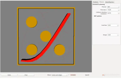
To show the result, in Figure 3.7 it has been used the recently created environ-ment in a Rigid Body robot 2D, a car, and the planner selected was RRT, for its interesting plotting outputs.
20 OMPL
Figure 3.6: 3D image generated by Blender of the environment required
Chapter 4
Planning Methods
Once we have seen how to develop any environment in OMPL through the dif-ferent way to do it, the next step is to choose which planner we want to use to solve our problem.
In OMPL there are two categories of planners:
• Geometric Planners • Control-based planners
In this chapter it will be discussed the different planning algorithms inside these two categories and how some of them work, the mainly used as RRT, PRM. Most of the planner have been developed in both categories, usually first came the geometric and then it was adapted to its control version. An exception of KPIECE, and PDST, which were create as control planner and then converted to geometric ones.
4.1
Geometric Planners
The planners in this category only accounts for the geometry and kinematics constraints of the system.
These geometric planners [3] compute a collision-free path connecting the initial and final configurations of a robot with a minimal number of waypoints, in 2D and 3D environments. As an output geometric planners provide a geometric description of the robot motion, the (x, y, z) coordinates of the path, given a validity checker function.
22 Planning Methods
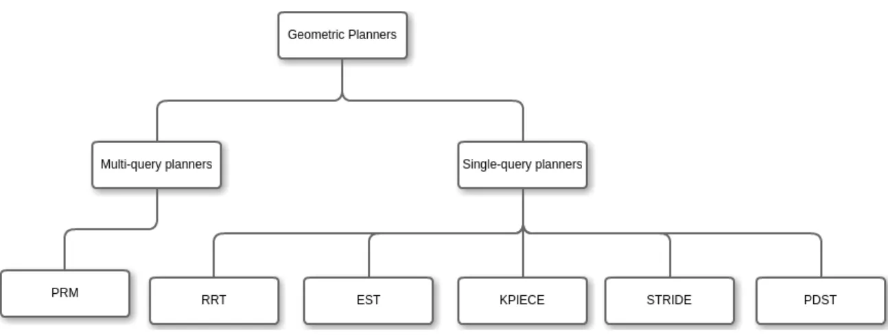
Figure 4.1: Classification of the two categories in geometric planners and all the planners inside them. Although, there is a third category which will be mentioned at the end of this chapter that is the optimizing planners
4.1.1
PRM
Probabilistic RoadMap, this planner is able to compute collision-free paths for robots of almost any type moving among static obstacles (fixed workspaces). But where PRM is very useful is for robots with many dof [4]. A general view of method has two phases:
• Roadmap phase: A roadmap the nodes of which are collision-free configu-rations and the edges are collision-free paths is built repeating two steps:
– Pick a random configuration of the robot, check it for collision and repeat this step until the slected configuration is collision-free.
– with a fast local planner, attempt to connect the former configuration to the roadmap. In Figure 4.2 we can see the final result of all these collision-free connections between the sampled states.
• Path creation phase: To find a path between an initial and goal configu-ration, this step attempts to connect these configurations to the roadmap and searches in the roadmap for a sequence of local paths linking them.
The name of multi-query planner is given because these two phases do not have to be executed sequentially. Instead, they can be mixed to limit or adapt the size of the roadmap to difficulties found during the path creation phase.
4.1 Geometric Planners 23
Figure 4.2: An example of a probabilistic roadmap after the first phase
Algorithm 3 Roadmap phase algorithm V ← ∅ E ← ∅ while |V | < n do repeat q ← a random configuration in Q until q is collision-free V ← V ∪ {q} end while for all q ∈ V do
Nq ← the k closest neighbours of q chosen from V according to dist
for all q0 ∈ Nq do if (q, q0) /∈ Eand M {(q, q0)} 6= N IL then E ← E∪ (q, q0) end if end for end for return G=(V,E)
In OMPL this planner has an implementation that uses one thread to con-struct a roadmap while a second thread checks whether a path exists in the roadmap between a start and goal state.
24 Planning Methods
The first phase can be seen in algorithm 3. It starts from an empty graph G = (V, E), then a randomly configuration q is chosen. If q is collision-free then is added to the graph and this process is repeated until N nodes are cre-ated, user’s choice. After that, the local planner, , connects q to q0 and if this connection is successful, meaning collision-free, is add as an edge.
Algorithm 4 Path selection phase algorithm
Nqinit ← the k closest neigbors of qinit according to dist
Nqgoal ← the k closest neigbors of qgoal according to dist
V ← {qinit} ∪ {qgoal} ∪ V
set q0 to be the closest neighbour of qinit in Nqinit
repeat
if M (qinit, q0) then
E ← (qinit, q0) ∪ E
else
set q0 to be the next closest neighbour of qinit in Nqinit
end if
until a connection was successful or the set Nqinit is empty
set q0 to be the closest neighbour of qgoal in Nqgoal
repeat
if M (qgoal, q0) then
E ← (qgoal, q0) ∪ E
else
set q0 to be the next closest neighbor of qgoal in Nqgoal
end if
until a connection was successful or the set Nqgoal is empty
P ← shortest path(qinit, qgoal, G)
if P is not empty then return P
else
return failure end if
While the procedure for the second phase it can be seen in Algorithm 4. This algorithm works having as an input an initial configuration, qinit, a goal
configuration qgoal, the number of closest neighbours to examine, k, and the
graph G, which is the output of the first stage. Once all the closest neighbours have been selected and added to Ninit and Ngoal, the algorithm starts checking
whether the path from closest one to qinit is free or not, in case is not free it will
continue with the next neighbour. Proceeding this way it could be sure that the path between qinit and qgoal will be the shortest, within the built roadmap. In
Figure 4.3 it can be seen the resulting path after both algorithms have been run and a path has been found. Among all the paths, in the roadmap, connecting
4.1 Geometric Planners 25
qinit with qgoal this is the shortest, however it is not the optimal one, for this case
it will be needed an optimizing planner.
Figure 4.3: Shortest path selected by PRM
Single-Query Planners What makes single query planners different from the multi-query ones is that the former are based on just one thread. These planner usually grows a tree of states connected by valid motions.
The differences among these planners are the approaches and techniques they use to control where and how tree is expand. Also, there are planner which involve the creation of two trees, in this case one from the start state and other from the goal state and the target of the planner attempts to find a node common to both trees, these planner are called bidirectional planners.
In this section we have selected the two more important algorithms to go deeper in them an later to analyse and compare one with each other: RRT, EST. Other algorithms like KPIECE or STRIDE are included in this category. How-ever, in the case of KPIECE, this will be touch in detail in the section of control-based planners since the first implementation was for dynamics systems.
4.1.2
RRT
A Rapidly-exploring Random Tree (RRT) is seen as an algorithm designed for searching in high-dimensional spaces, but is also a structure where data of each single configuration is saved. RRTs are built incrementally, in such a way that the distance between the random sampled state to the tree is reduced quickly. RRTs are very suitable for motion planning problems involving obstacles and, subjected to differential constraints. RRTs can be considered as a technique for
26 Planning Methods
Figure 4.4: Tree created with RRT
generating open-loop trajectories for non-linear systems specific constraints [5]. Usually, an RRT alone is not enough to solve a planning problem. That is why, it could be interesting to consider it as a component or as a module that can be used for the development of a wide variety of different planning algorithms. A brief description of the method for a general configuration space C (this could be a state space with defined position and velocity).
Algorithm 5 RRT2
1: V ← {xinit; E ← ∅
2: for i = 1, ..., n do
3: xrand→ SampleFree;
4: xnearest← NEAREST(G=(V,E),xrand);
5: xnew ← Steer(xnearest, xrand);
6: if Obstaclefree(xnearest, xrand) then
7: V ← V ∪ {xnew}; E ← E ∪ {(xnearest, xnew)
8: end if
9: end for
10: return G=(V,E)
The function add_edge includes a local planner responsible to check whether qrand is colliding with the obstacles, Cobs, or not, Cf ree.
An example of the previous algorithm is shown in Figure 4.4, where it could be seen the tree generated in whole free space avoiding the obstacles, blue circles. However this is a very simple example, and the problem could become more and more complex as we try to approach some real situations.
4.1 Geometric Planners 27
Figure 4.5: RRT
RRTconnect Inside OMPL we can find a version of RRT which applies the al-gorithm twice, one from the star and other from the goal, a bidirectional version of RRT. In the next example, shown in Figure 4.5 we have a car that has to go from the bottom part of the map to the top while avoiding some small obstacles and a big one in the top left part that creates kind of narrow passage. In order to solve this problem, a modification of RRT has been done, which is basically the use of two trees, one rooted at goal state and other at start state and whit the objective to find a common node to both trees and connect them.
The RRT based algorithms have several properties that make them very suit-able for a wide variety of planning problems: 1) the expansion of the RRT is pushed toward parts of the state space still unexplored; 2) The distribution of the vertices in an RRT approaches the sampling distribution (gaussian, uniform...); 3) an RRT is probabilistic complete under very general conditions; 4) as the PRM, the RRT algorithm is relatively simple, which facilitates performance analysis; 5) an RRT is always connected, even if the number of nodes is small; 6) an RRT can be used as a module, and could be adaptable and flexible, which provides a wide variety of planning systems.
A consequence of this might be that RRTs could be faster that PRM for holo-nomic plannning problems since as mentioned in the advantage 5), RRT remains connected with a few number of edges while PRM creates many extra edges in
28 Planning Methods
Figure 4.6: Visibility region
the creation of the roadmap.
4.1.3
EST
EST, Expansive Space Trees, is a tree-based motion planner that attempts to detect the less explored areas of the space through the use of a grid imposed on a projection of the state space. Using this information, EST continues tree expan-sion primarily from less explored areas. As PRM, it is also based on a roadmap of milestones sampled in the free region of the configuration space. The differ-ence with PRM relies in that this new algorithm tries to expand the roadmap only in the direction that is interesting for the pursued solution [6], meaning the part that contains only the configurations that are connected either to the ini-tial configuration qinit or the goal configuration qgoal, avoiding the extra work of
computing the roadmap for the whole configuration space. To accomplish this requirement the idea is to star sampling in the neighbours of qinit and qgoal, and
then new samples in the neighbours of those which it is known to be connected to qinit and qgoal, until a path is found. In order to have the ability to construct
this dirigible roadmap the concept of visibility set is defined, let V(p) be the set of all configurations seen from a free state p. In figure 4.6 are shown the two trees, blue one and white one, and surrounding each node there is a close are, which represents the visibility region.
The algorithm of EST works as follows: given two configurations qinit and
4.1 Geometric Planners 29
path-connected to either qinit or qgoal. After that, two trees are built rooted on
both, initial and goal, configurations. These two tree are grown until the visibility region of one intersects with the visibility region of the other. The algorithm has basically two steps, expansion and connections, as shown in algorithms 7 and 6. A key point of this algorithm resides in the concept of weight of x, w(x), which is defined as the number of sampled nodes inside Nd(x) [6]. This means that
regions with few nodes have more probability to be sampled. Algorithm 6 Expansion step
pick node x from V with probability 1/ω(x) sample K point from Nd = {q ∈ C|distc(x, q) < d}
for each configuration y that has been picked do
calculate ω(y) and retain those y with probability 1/ω(y)
if y is retained and clearance(y)>0 and link(x, y) returns YES then put y in V and place and edge between x and y.
end if end for
Algorithm 7 Connection step
for every x ∈ Vinit and every y ∈ Vgoal do
if distw(x, y) < l then
link(x, y) end if end for
4.1.4
Optimizing Planners
However, as mentioned before the increasingly relevance of this algorithms to be applied in any aspect of the life made sometimes them very useful but not enough to accomplish some requirements in terms of accuracy or path length, or any other feature likely to be optimized. That is the reason which motivated the development of the optimization algorithms, versions of the already created RRT or PRM, with the difference that the result is given as an optimization of some of the aspects in the planning problem.
In OMPL, for example, two main different optimization objectives have been implemented.
• Path Length: The goal of this optimization objective is to find the shortest collision-free path possible. See Figure 4.7 a).
• Maximum clearance: This objective, for safety reason for example, tries to steer the robot away from the obstacles. See Figure 4.7 b).
30 Planning Methods
(a) Path Length optimization objective (b) Maximum clearance optimization objec-tive
Figure 4.7: Optimization objectives
More optimization objective have been created but they are combination of the two seen above such as: Balanced Optimization, which optimizes a trade-off between path length and maximum clearance by giving them some weight and summing them; Maximize minimum clearance, that is the cost of a given path is only function of the closest distance between the path and a obstacle.
RRT* In order to reach the RRT* that ensures an optimal solution first we have to mention the RRG (Rapidly-exploring Random Graph).
The Rapidly-exploring Random Graph algorithm was introduced as an in-cremental algorithm to build a connected roadmap, possibly containing cycles. The RRG algorithm is similar to RRT. As RRT,it firstly attempts to link the nearest node to the new sampled state. If that connection is successful, the new node is added to the vertex structure. However, RRG is different is the following. Each time a new state xnew is added to the vertices V , then
con-nections are tried from all other vertices in V that are within a ball of radius r(card(V ))= min(γRRG(log card(V )/card(V ))1/d, η), where η is the constant
ap-pearing in the definition of the local steering function [7], and γRRG > γRRG∗ =
2(1+1/d)1/d(µ(Xf ree)/ς
d)1/d . For each successful connection, a new edge is
added to the edge set E. Hence, it could be said that the RRT graph (a directed tree) is a subgraph of the RRG graph (an undirected graph). The two graphs share the same vertex set, and the edge set of the RRT is a subset of that of the RRG. Another version of the algorithm, called k-nearest RRG, can be consid-ered, in which connections are not attempted inside a ball but are limited to k nearest neighbours, with k = k(card (V )) := kRRGlog(card(V )), where kRRG >
kRRG = e(1 + 1/d), and Xnear ←kNearest(G = (V, E), xnew, kRRGlog(card(V ))),
in line 7 of Algorithm 8. A computational advantage of this second method is that kRRG is a constant that depends only on d, and does not depend on the
4.1 Geometric Planners 31
configuration space, unlike γRRG∗ . Moreover, kRRG = 2e is a valid choice for all
problem instances.
Algorithm 8 RRG
1: V ← xinit; E ← ∅ ;
2: for i = 1, ..., n do
3: xrand ← SampleF reei;
4: xnearest← N earest(G = (V, E), xrand);
5: xnew ← Steer(xnearest, xrand);
6: if ObstacleFree(xnearest, xnew) then
7: Xnear ← N ear(G = (V, E), xnew, min(γRRG(log card(V )/card(V ))1/d, η));
8: V ← V ∪ xnew; E ← E ∪ (xnear, xnew), (xnew, xnear);
9: for xnear ∈ Xnear do
10: if CollisionFree(xnear, xnew) then
11: E ← E ∪ (xnear, xnew), (xnew, xnear);
12: end if
13: end for
14: end if
15: end for
16: return G=(V,E);
The RRT∗ algorithm is obtained by modifying RRG, removing those edged that are redundant due to the cycles formed during the algorithm is run. RRT and RRT∗ graphs are directed trees with the same root and vertex set, and edge sets that are subsets of that of RRG, this creates the necessity to a "rewiring" of the RRT tree, in orde to ensure that the nodes are reached through a minimum-cost path.
Before discussing the algorithm, it is necessary to introduce a few new functions. Given two points x1, x2 ∈ <d , let Line(x1, x2) : [0, s]X denote the
straight-line path from x1 to x2. Given a tree G = (V, E), let P arent : V → V be
a function that maps a vertex v ∈ V to the unique vertex u ∈ V such that (u, v) ∈ E. By convention, if v0 ∈ V is the root vertex of G, P arent(v0) = v0.
Finally, let Cost : V <0 be a function that maps a vertex v ∈ V to the cost
of the unique path from the root of the tree to v. For simplicity, in stat-ing the algorithm we will assume an additive cost function, so that Cost(v) = Cost(P arent(v)) + c(Line(P arent(v), v)), although this is not necessary for the analysis in the next section. By convention, if v0 ∈ V is the root vertex of G,
then Cost(v0) = 0.
The RRT algorithm adds points to the vertex set V in the same way as RRT and RRG. It also considers connections from the new vertex xnew to vertices in Xnear,
i.e., other vertices that are within distance r(card(V )) = minγRRT∗ (log(card(V ))/card(V ))1/d, η
in-32 Planning Methods
serted in the edge set E. In particular, (i) an edge is created from the vertex in Xnear that can be connected to xnew along a path with minimum cost, and (ii)
new edges are created from xnew to vertices in Xnear, if the path through xnew
has lower cost than the path through the current parent; in this case, the edge linking the vertex to its current parent is deleted, to maintain the tree structure. As happened with RRG, another version of the algorithm, called k-nearest RRT∗, can be considered, in which connections are sought to k nearest neighbors, with k(card(V )) = kRRGlog(card(V )), and Xnear ← kN earest(G = (V, E), xnew, kRRGlog(i)),
in line 7 of Algorithm 9. Algorithm 9 RRT*
1: V ← xinit; E ← ∅ ;
2: for i = 1, ..., n do
3: xrand← SampleF reei;
4: xnearest← N earest(G = (V, E), xrand);
5: xnew← Steer(xnearest, xrand);
6: if ObstacleFree(xnearest, xnew) then
7: Xnear ← N ear(G = (V, E), xnew, min(γRRG(log card(V )/card(V ))1/d, η));
8: V ← V ∪ xnew;
9: xmin ← xnearest; cmin ← Cost(xnearest) + c(Line(xnearest, xnew));
10: for xnear ∈ Xnear do
11: if CollisionFree(xnear, xnew) ∧Cost(xnear)+c(Line(xnear, xnew)) < cmin
then
12: xmin ← xnear; cmin ← Cost(xnear) + c(Line(xnear, xnew));
13: end if
14: end for
15: E ← E ∪ (xmin, xnew);
16: for xnear ∈ Xnear do
17: if CollisionFree(xnew, xnear) ∧Cost(xnew) + c(Line(xnew, xnear)) <
Cost(xmin) then
18: xparent ← P arent(xnear)Cost(xnear) + c(Line(xnear, xnew));
19: end if
20: E ← E (xparent, xnear) ∪ (xnew, xnear);
21: end for
22: end if
23: end for
24: return G=(V,E);
PRM* In standard PRM algorithm connections are attempted between roadmap vertices that are within a fixed radius r from one another. In PRM* instead the connections radius r is chosen as a function of n, r=r(n):=γP RM(log(n)/n)1/d,
4.2 Control-based Planners 33
where γP RM > γP RM∗ = 2(1 + 1/d)
1/d(µ(X
f ree)/ςd)1/d, d is the dimension of the
space X, µ(Xf ree) denotes volume of the obstacle-free space. In this way the
connection radius decrease with the number of sample. Algorithm 10 PRM*
V ← {xinit} ∪ { SampleFreei}i=1,....,n; E ← ∅
for all v ∈ V do
U ← Near(G = (V, E), v, γP RM(log(n)/n)1/d) {v};
for all u ∈ U do if CollisionFree(v, u) then E ← E ∈ {(v, u), (u, v)} end if end for end for return G=(V,E)
In algorithm 10 it can be seen the procedure of PRM*. Once the milestones of the roadmap have been sampled. All the connections from the v node to the nodes inside the radius neighbour r are checked. If this connection is collision-free the edge from u to v is created and added to the path. With this procedure, as the number of samples increases the connection radius decreases, since the sampling phase and the connection phase are launched simultaneously, it can be ensured that the final path connecting an xinit and xgoal will be optimal.
4.2
Control-based Planners
If the considered system is subject to differential constraints, then a control-based is used. In OMPL these planners rely on the State Propagator was mentioned in Section 2, instead of a simple interpolation to generate motions. While the output solving a problem with a geometric planner is a series of point expressing the geometric configuration, i.e. the coordinates in the state space, in the control planners instead, the output will be a series of point in which are expressed the geometric coordinates, because actually is what determines the path, but also the control inputs, as much as have been defined, and the duration of such inputs.
In Figure 4.8 we can observe a piece of the output printed when running a problem with a control-based planner. In this specific case it was defined a SE2 state space, (x, y, θ), and two control input. In the matrix printed we find the first three columns as the coordinates, for plotting reasons, but what determine this coordinates is the control inputs printed in columns 4 and 5 and its duration, last column.
In this section we will focus on the description of KPIECE, although in this category we can find also other planner like PDST and the control based version
34 Planning Methods
Figure 4.8: Output of a control planner
of RRT and EST,these two are the same as its geometric version already explained in the previous section, but with the extra ability of expressing the path as a function of the control and durations. In the case of PDST is a planner developed in OMPL to solve very specific situations and in this thesis we prefer to focus on more generic situations.
4.2.1
KPIECE
Kinodynamic motion Planning Interior-Exterior Cell Exploration, specifically de-signed for systems with complex dynamics. KPIECE has some particular features as it does not require state sampling or distance metric. However, it requires a projection of the state space and the specification of a discretization, as was made in [8].
An instance of the motion planning will be formulated as S = (Q, U, I, F, f ), where Q is the state space, U the control space, I the set of initial configurations, F the set of final configurations, and f the propagation function.
In algorithm 11 is shown how this algorithm works. In which, c cell chain is understood as a k connected cells in a row, and it has decided to expand from the interior to exterior, reason to use the bias in line 5. Once a state s has been chosen from the motion µ, the tree is expanded from s checking for a valid motion depending on t. If some motion collision free has been found and the tree could be expanded through it, the new motion is added to the tree of motions. Then it is needed to recalculate the discretization. After that for each level of discretization a the progress Pj is calculated with some increase ratio in the coverage given by
the increase in coverage of p. Pj is used as a penalty if not enough progress has
been made by the multiplication of pj.
The AddMotion procedure shown in algorithm 12, first of all divide the motion into submotions so as to avoid that any of the motions collide with the boundary of any cell. Then for all this submotions the algorithm has to find the cell chain
4.2 Control-based Planners 35
Algorithm 11 KPIECE(qstar, Niterations)
1: Let µ0 be the motion of the duration 0 containing only qstart
2: Create an empty Grid data-structure G
3: G.AddMotion(µ0)
4: for i ← 1....Niterations do
5: Select a cell chain c from G, with bias on exterior cells (70% − 80%)
6: Select µ from c according to a half normal distribution 7: Select s along µ
8: Sample random control u ∈ U and simulation time t ∈ R+
9: Check if any motion (s, u, to), to ∈ (0, t] is valid (forward propagation)
10: if a motion is found then
11: Construct the valid motions µo =(s, u, to) with to maximal
12: if µo reaches the goal region,
13: return path to µo
14: G.AddMotion(µo)
15: end if
16: for every level Lj do
17: Pj = α + β · (ratio of increase in coverage of Lj to simulated time)
18: Multuply the score of cell pj in c by Pj if and only if Pj < 1
19: end for
20: end for
Algorithm 12 AddMotion(s, u, t)
1: Split (s, u, t) into motions µ1, ..., µksuch that µidoes not cross the boundary
of any cell at the lowest level of discretization
2: for µo ∈ {µ1, ..., µk} do
3: Find the cell chain corresponding to µo
4: Instantiate cells in the chain, if needed
5: Add µo to the cell at the lowest level in the chain
6: Update coverage measures and lists of interior and exterior cells, if needed
36 Planning Methods
Figure 4.9: Problem planning of a maze with an unique solution
which they belong to, and add this submotion at the lowest level of the chain. Once it has been added it has to update the coverage since it will be necessary to compute the progress in the following step of algorithm 11 and the list of internal and external cells, is something has changed.
to provide an example of a problem solve with this algorithm in figure 4.9 we can observe there are two colors of edges. Each color corresponds to each level of discretization Lj. In this case in OMPL the algorithm KPIECE has been
implement with two levels of discretization. The first one is represented in Figure 4.9 with the blue color, while the second level of discretization es the green one.
Chapter 5
Comparative experiments
In the previous chapter the main different algorithms used in OMPL to solve motion planning problems have been explained in detail: how they work, which technique they are approached with, how their outputs are given and the different existing categories.
However, it would be useful to have a common view of all of them, so as to make easier the decision of which one suits better with the necessity based on their features and the data obtained from the experiments.
To do so we are going to run the same planning problem, the one described in section 2. But subtly changed in order to adapt it to the specific situation. For geometric planners it will be elaborated a comparison between the geometric ver-sion of RRT, PRM, EST and KPIECE.
In the case of control-based planner, the same environment as the same robot will be used but a state propagator must be added, according to de dynamics of the selected car. And the planners selected are RRT, PRM and EST.
In the end, there will be three comparisons among the optimizing planners, two involving the non-optimized version of RRT and PRM against their optimized versions and the last one will rely on the comparison between the two optimizing planners RRT* and PRM*.
In the next sections the data shown in the tables are: time to find a solution, number of states sampled, number of states in the path, length of the path and number of edges for each one of the geometric planners. All this data are given in average, since we are working with randomized planner one experiment could differ too much from other simply because they are based on random samplings, that is why in order to give a general view of the data obtained, for each planner the experiment have been done ten times and from those ten experiments the average of time, number samples, states conforming the path, path length and created edges, was calculated.
38 Comparative experiments Table 5.1: Geometric planners
RRT PRM KPIECE EST Time (ms) 1,29 5,22 1,25 1,53 Samples 35 68 52 92 Path states 8 5 12 6 Cost (length) 146 121 236 161 Edges 34 1067 51 91
5.1
Geometric Planners
In Table 5.1 it can be seen how some parameters change according to the planner is used to solve a specific problem.
If we first focus on the time spent to find a solution, we can see that, except PRM the rest of them have a similar response around 1.5 ms. The fact that PRM has a solution time much higher, even if we are speaking about miliseconds the response is four times larger than in the others, is due to the way of proceed of this planner. As was commented in the previous chapter, PRM samples a milestones which are then connected one each other within a neighbour radius. That task produces an extra effort which implies an increment of the time. To confirm this it must look at the last row in table 5.1 where it can be seen the huge difference between the edges creates by PRM and the edges created by the others, more than ten times.
In order to give some graphic example to allow us to observe this difference we have taken one of those ten experiments run for each planner and we have plotted. In Figure 5.1 we can observe how the environment (b), is almost full of edges, all those extra edges computed by PRM.
The numbers of samples created by the planners gives as an idea of how fast each planner can explore the configuration space. We can evaluate the sampling rate as the number of states sampled per second. In this case we can see a higher value of the sampling rate for the EST planner due to that the expansion step of this planner is done by building two tree one from qinit and one from qgoal, so it
is straightforward to say that is doubling the rate of the others.
The two factors left are commented together since looking at the table we can see a proportional relation between the number of states conforming the path, and the length of such path, the less number of states, the shorter is the path, not always though. First thing we should remark is the big difference between KPIECE and the others. However, this is because KPIECE was designed to work properly in systems with very complex dynamics, and using it to solve a basic planning problem like ours makes it loosing efficiency. As the complexity of the systems increase KPIECE becomes more suitable. Something similar happens with EST, as it is designed to go towards part of the space unexplored, in this
5.2 Control Planners 39
case we know from where to where we want to arrive, so as its colleague losses some power while exploring parts of the map that are not interesting.
5.2
Control Planners
In order to elaborate a complete comparison between the control planner, we must remark the fact that in geometric planners the planner termination con-ditions indicates that in case a solution is found the planner stop running and that solution is given as path. In the case of control-based planners when we implemented the code, in the moment of make the call to the function solve() for each planner, we set the time within the planner has to try to find a solution. For our experiment this time was set to 1 second since is a period of time in which all the planner were able to find a solution, reducing this set time produced that not always and not every planner found a solution path. That is the reason the mean time to find a solution shown in the table 5.2 is quite close to one for the three of them.
As a consequence of the definition of control path, that is a path determined by a set of control inputs along with the duration of such inputs, the trajectories generated by the planner won’t be straight lines. This consequence produces an opposite effect to the pattern seen in the previous section where we had a proportional relationship between states of the path and length of the path, while in this case this relation is inversely proportional. In other words, as we are dealing with curved trajectories, the more and smaller curves, the less path length.
As happened with the geometric planner the sampling rate of EST is much bigger than the other planners due to its two tree growing. In this case that difference is even bigger because as the time increases the number of nodes from which the tree can grow increases and the number samples is not just the doble but it has an exponential increase.
Regarding the last term, the number of edges, as in this sections we are dealing with control planner and all of them are tree-based planners, the tree is always grown in one direction in the sense that from one single node there is just one edge arriving and one edge starting so at the end in tree-based algorithms the number of edges will be always one unit less than the sampled nodes.
Apart from the information provided in table 5.2, a graphical representation of the three algorithms has been made in figure 5.2. It is shown here the great difference in the number of edges of EST with the other two methods. It is also remarkable how in this case, with a dynamic car as was mentioned before, KPIECE works better than in the geometric case, in fact is the one providing the shortest path. Even if the dynamics of the systems are not very complex we can state that KPIECE is a good alternative as long as as the considered system is subjected to dynamical constraints.
40 Comparative experiments
(a) RRT (b) PRM
(c) KPIECE (d) EST
Figure 5.1: Geometric planners: paths and edges
Table 5.2: Control planners
RRT KPIECE EST Time 1,008 1,007 1,007 Samples 15552 30980 166020 Path states 146 221 47 Cost (length) 363 313 339 Edges 15551 30979 166019
5.2 Control Planners 41
(a) RRT (b) EST
(c) KPIECE
42 Comparative experiments
5.3
Optimizing Planners
In this section three comparison will be elaborated regarding optimizing planners. In OMPL we have as optimal planner PRM* and RRT*. First we are going to check that they are really giving an optimal solution against their non-optimized version, in both cases. After that we will attempt to decide which optimal planner gives the best solution.
As happened in the previous section, with the preset window time to find a solution, when dealing with optimazing planners, these are designed to be probabilistic completes, meaning that if we let the planner running infinite time it will provide an optimal solution in almost 100% of the cases. Even if it finds a solution the planner termination condition is not set so will keep refining the solution infinitely. That is why we have two options here, we can either limit the window time within the planner has to find a solution, or limit the number of nodes. Since here we are dealing with a basic planning problem, for the geometric planner will not take a large number of states to reach a solution, so it does not make sense to limit the number of nodes for the optimized version. We decided to limit the time as in the previous situation.
5.3.1
RRT vs RRT*
First remarkable difference we can observe in Table 5.3 is the time needed to find a solution. As we mentioned before the time for the optimizing planner was predefined in order to limit somehow the planner termination condition.
The sampling rate instead is approximately the same. The small number of sampled states is because of it quickly finds a solution. So in terms of computa-tional effort both planner are similar.
Then, the key point when considering optimizing planning is the thing we want to optimize. In our case it was selected the default optimization objective, path length. If we look at the 4th row in table 5.3 we can confirm that RRT* gets an optimal solution. To give shape to these data in figure 5.3 we can see the path provided by RRT* while in figure 5.1 a) was represented RRT. The fact that RRT* path is represented like a composition of straight lines it is an indicator of its optimality since it is known that the shortest path between two point is a straight line.
5.3.2
PRM vs PRM*
In the case of probabilistic road map, the difference between the optimizing ver-sion and the non-optimizing is that in the second phase of the algorithm, con-nection phase, the neighbour radius, in which the algorithm looks for nodes to connect to, is not constant but given as a function of the number of samples
5.3 Optimizing Planners 43 Figure 5.3: RRT* Table 5.3: RRT vs RRT* RRT RRT* Time (ms) 1,29 1001 Samples 35 20665 Path states 8 14 Cost (length) 146 119 Edges 34 20665
44 Comparative experiments Table 5.4: PRM vs PRM* PRM PRM* Time (ms) 5,22 1001 Samples 68 8641 Path states 5 13 Cost (length) 121 118 Edges 1067 398769
nodes. More specifically, the radius decreases as the number of sampled states increases.
In the case of the optimizing planner we find the value of 1 second that was establish in the setup stage. Even if the PRM has higher response than other geometric algorithms, in table 5.4 the difference between times is a big gap. For the sampling rate we can observe similar values. This happens because the first phase of the algorithm is the same, sampling a certain number of milestones in the free space.
The remarkable difference is the generation of the edges, i.e. the connection stage, while in PRM is constant in PRM* is decreasing with the time which allows a reduction of the computational effort.
The path length in this specific problem is approximately the same, so it is not a determinant factor when making the decision.
5.3.3
RRT* vs PRM*
The comparison between RRT* and PRM* is analogue to the one made fore their non-optimizing version. That is why to give some different approach, this time we have introduced the other limitation mentioned before, the maximum number of nodes, while keeping the time always as 1 second.
This modifications does not change the numbers of the column PRM*, in table 5.5 since the limit is not reached but it does with the RRT*.
In this case taking into account the data given in the table we can note that RRT* is quicker even if the sampling rate is smaller.
With respect to the path length as both are optimal, this difference is negligible. It has been demonstrated that they give an optimal solution, so this could not be improved.
The last aspect is the number of created edges, close to 40 times bigger in the case of PRM*, that is the reason that makes it slower than RRT*.
5.3 Optimizing Planners 45 Table 5.5: RRT* vs PRM* RRT* PRM* Time (ms) 364,3 1001 Samples 9999 8641 Path states 16 13 Cost (length) 118,73 118 Edges 9999 398769
Chapter 6
Conclusion
As a conclusion of all commented in the previous chapter regarding the geometric planner, we can say that for this specific case scenario KPIECE and EST could be rejected. Then making a decision about RRT or PRM will depend on some external constrains as for example the time, if it’s an important factor although PRM gives shorter paths, takes more time. In that point is up to the user to decide which are the requirements and how to use them.
With respect to the control planners, we have to start considering the use of KPIECE for such problems, even if it was designed for more dynamical complex problems, it already provides a feasible solution with a cost smaller than the other methods. Maybe this is a consequence of the fact that KPIECE was first developed for problems involving dynamical constraints and then converted to its geometric version.
Again, depending on the requirements the user is asked for, he will have to decide whether using one planner or other regarding what is more relevant if the path length, in such case the candidate will be KPIECE, or it attempts to reduce the computational effort, which is lower in the case of RRT.
When dealing with optimizing planners from our first experiment RRT vs RRT* we get the conclusion that if the user needs a path planning high-ended, with a level of accuracy relevant, the most suitable is RRT*. While if the necessity just implies a path between two point RRT suits better since is at least 100 times quicker.
In the case of PRM and PRM* there are two factor with enough relevance to consider them when making the decision about what planner will be use: the time and the computational effort. And one excludes each other since if you prefer a quick solution rather than an optimal, PRM is the chosen. In the opposite case, shortest path is pursued PRM*,but spending more time.
In the last case scenario, RRT* vs PRM*, with the data obtained, we can conclude that in this kind of problems is RRT* is better in all the relevant aspects: quicker and less computational effort.
Bibliography
[1] H. CHOSET, “Robotic motion planning: Cell decompositions,”
[2] Y. Hwang and N. Ahuja, “A potential field approach to path planning,” IEEE Transactions on Robotics and Automation, vol. 8, 1992.
[3] Z. ALJARBOUA, “Geometric path planning for general robot manipulators,” Proceedings of the World Congress on Engineering and Computer Science, vol. 02, 2009.
[4] L. Kavraki, P. Svestka, J.-C. Latombe, and M. Overmars, “Probabilis-tic roadmaps for path planning in high-dimensional configuration spaces,” Robotics and Automation, IEEE Transactions on, vol. 12, pp. 566–580, Aug 1996.
[5] J. Kuffner and S. LaValle, “Rrt-connect: An efficient approach to single-query path planning,” in Robotics and Automation, 2000. Proceedings. ICRA ’00. IEEE International Conference on, vol. 2, pp. 995–1001 vol.2, 2000. [6] D. HSU, J.-C. LATOMBE, and R. MOTWANI, “Path planning in
expan-sive configuration spaces,” International Journal of Computational Geometry amp; Applications, vol. 09, no. 04n05, pp. 495–512, 1999.
[7] S. Karaman and E. Frazzoli, “Sampling-based algorithms for optimal motion planning,” CoRR, vol. abs/1105.1186, 2011.
[8] I. SUCAN, “kinodynamic motion planning by interior-exterior cell explo-ration,”
[9] S. LA VALLE, “Rapidly-exploring random trees: A new tool for path plan-ning,”
List of Figures
2.1 Probabilistic roadmap . . . 13
2.2 RRT . . . 13
2.3 Trapezoidal Decomposition . . . 13
3.1 Overview of the OMPL framework . . . 16
3.2 Robot Selection . . . 19
3.3 Environment selected . . . 19
3.4 Full configuration:robot, environment, start and goal . . . 19
3.5 Solution path and edges generated . . . 19
3.6 3D image generated by Blender of the environment required . . . 20
3.7 Output of the planning motion in ompl.app with our own environ-ment . . . 20
4.1 Classification of the two categories in geometric planners and all the planners inside them. Although, there is a third category which will be mentioned at the end of this chapter that is the optimizing planners . . . 22
4.2 An example of a probabilistic roadmap after the first phase . . . . 23
4.3 Shortest path selected by PRM . . . 25
4.4 Tree created with RRT . . . 26
4.5 RRT . . . 27
4.6 Visibility region . . . 28
4.7 Optimization objectives . . . 30
4.8 Output of a control planner . . . 34
4.9 Problem planning of a maze with an unique solution . . . 36
5.1 Geometric planners: paths and edges . . . 40
5.2 Control planners: paths and edges . . . 41
List of Tables
5.1 Geometric planners . . . 38 5.2 Control planners . . . 40 5.3 RRT vs RRT* . . . 43 5.4 PRM vs PRM* . . . 44 5.5 RRT* vs PRM* . . . 45Chapter 7
Appendix
.1
Example.cpp
#i n c l u d e <ompl / b a s e / PlannerData . h> #i n c l u d e <ompl / b a s e / P l a n n e r D a t a S t o r a g e . h> #i n c l u d e <ompl / b a s e / PlannerDataGraph . h> #i n c l u d e <ompl / b a s e / s p a c e s / S E 3 S t a t e S p a c e . h> #i n c l u d e <ompl / b a s e / o b j e c t i v e s / P a t h L e n g t h O p t i m i z a t i o n O b j e c t i v e . h> #i n c l u d e <ompl / g e o m e t r i c / p l a n n e r s / r r t / RRTstar . h> #i n c l u d e <ompl / g e o m e t r i c / p l a n n e r s / r r t /RRT. h> #i n c l u d e <ompl / g e o m e t r i c / p l a n n e r s /prm/PRMstar . h> #i n c l u d e <ompl / g e o m e t r i c / p l a n n e r s /prm/PRM. h> #i n c l u d e <ompl / g e o m e t r i c / p l a n n e r s / e s t /EST . h> #i n c l u d e <ompl / g e o m e t r i c / p l a n n e r s / k p i e c e /KPIECE1 . h> #i n c l u d e <ompl / g e o m e t r i c / S i m p l e S e t u p . h> #i n c l u d e <ompl / b a s e / g o a l s / G o a l S t a t e . h> #i n c l u d e <b o o s t / graph / a s t a r _ s e a r c h . hpp> #i n c l u d e <i o s t r e a m > namespace ob = ompl : : b a s e ; namespace og = ompl : : g e o m e t r i c ; b o o l i s S t a t e V a l i d ( c o n s t ob : : S p a c e I n f o r m a t i o n ∗ s i , c o n s t ob : : S t a t e ∗ s t a t e ) { // ob : : S c o p e d S t a t e <ob : : SE2StateSpace> // c a s t t h e a b s t r a c t s t a t e t y p e t o t h e t y p e we e x p e c t c o n s t ob : : R e a l V e c t o r S t a t e S p a c e : : StateType ∗ s t a t e 2 d = s t a t e −> as<ob : : R e a l V e c t o r S t a t e S p a c e : : StateType > ( ) ;56 Appendix
d o u b l e x = s t a t e 2 d −>v a l u e s [ 0 ] ; d o u b l e y = s t a t e 2 d −>v a l u e s [ 1 ] ;
r e t u r n s i −>s a t i s f i e s B o u n d s ( s t a t e ) && ( x − 7 5 . ) ∗ ( x −75.)+( y − 2 5 . ) ∗ ( y −25.) >100. && ( x − 2 5 . ) ∗ ( x −25.)+( y − 2 5 . ) ∗ ( y −25.) >100. && ( x − 2 5 . ) ∗ ( x −25.)+( y − 7 5 . ) ∗ ( y −75.) >100. && ( x − 5 0 . ) ∗ ( x −50.)+( y − 5 0 . ) ∗ ( y − 5 0 . ) > 1 0 0 . ; // r e t u r n s i −>s a t i s f i e s B o u n d s ( s t a t e ) ; } v o i d p l a n W i t h S i m p l e S e t u p ( v o i d ) { // c o n s t r u c t t h e s t a t e s p a c e we a r e p l a n n i n g i n ob : : S t a t e S p a c e P t r s p a c e ( new ob : : R e a l V e c t o r S t a t e S p a c e ( 4 ) ) ; // s e t t h e bounds f o r t h e R^3 p a r t o f SE ( 3 ) ob : : RealVectorBounds bounds ( 4 ) ; bounds . low [ 0 ] = 0 . ; bounds . low [ 1 ] = 0 . ; bounds . h i g h [ 0 ] = 1 0 0 . 0 ; bounds . h i g h [ 1 ] = 1 0 0 . 0 ; bounds . low [ 2 ] = − 3 . 1 4 ; bounds . h i g h [ 2 ] = 3 . 1 4 ; bounds . low [ 3 ] = 0 . 0 0 1 ; bounds . h i g h [ 3 ] = 1 . ;
s p a c e −>as<ob : : R e a l V e c t o r S t a t e S p a c e >()−>se tBo un ds ( bounds ) ; // d e f i n e a s i m p l e s e t u p c l a s s og : : S i m p l e S e t u p s s ( s p a c e ) ; // s e t s t a t e v a l i d i t y c h e c k i n g f o r t h i s s p a c e s s . s e t S t a t e V a l i d i t y C h e c k e r ( b o o s t : : b i n d (& i s S t a t e V a l i d , s s . g e t S p a c e I n f o r m a t i o n ( ) . g e t ( ) , _1 ) ) ; ob : : S c o p e d S t a t e <ob : : R e a l V e c t o r S t a t e S p a c e > s t a r t ( s p a c e ) ; s t a r t [ 0 ] = 1 0 . 0 ; s t a r t [ 1 ] = 1 0 . 0 ; s t a r t [ 2 ] = 0 . ; s t a r t [ 3 ] = 0 . 0 0 2 ; // c r e a t e a g o a l s t a t e ob : : S c o p e d S t a t e <ob : : R e a l V e c t o r S t a t e S p a c e > g o a l ( s t a r t ) ; g o a l [ 0 ] = 9 0 . 0 ; g o a l [ 1 ] = 9 0 . 0 ;
.1 Example.cpp 57 g o a l [ 2 ] = 0 . 0 ; g o a l [ 3 ] = 0 . 5 ; // s e t t h e s t a r t and g o a l s t a t e s s s . s e t S t a r t A n d G o a l S t a t e s ( s t a r t , g o a l , . 0 5 ) ; s s . s e t P l a n n e r ( ob : : P l a n n e r P t r ( new og : : PRMstar ( s s . g e t S p a c e I n f o r m a t i o n ( ) ) ) ) ;
// t h i s c a l l i s o p t i o n a l , but we put i t i n t o g e t more o u t p u t i n f o r m a t i o n s s . s e t u p ( ) ; s s . p r i n t ( ) ; // attempt t o f i n d an e x a c t s o l u t i o n w i t h i n f i v e s e c o n d s // i f ( s s . s o l v e ( 1 0 . 0 ) == ob : : P l a n n e r S t a t u s : : EXACT_SOLUTION) i f ( s s . s o l v e ( 1 0 . 0 ) ) { // s s . s i m p l i f y S o l u t i o n ( ) ; og : : PathGeometric s l n P a t h = s s . g e t S o l u t i o n P a t h ( ) ; s t d : : c o u t << s t d : : e n d l ; s t d : : c o u t << "Found s o l u t i o n w i t h " << s l n P a t h . g e t S t a t e C o u n t ( ) << " s t a t e s and l e n g t h " << s l n P a t h . l e n g t h ( ) << s t d : : e n d l ; // p r i n t t h e path t o s c r e e n s l n P a t h . p r i n t A s M a t r i x ( s t d : : c o u t ) ; s t d : : c o u t << " W r i t i n g PlannerData t o f i l e ’ . / myPlannerData ’ " << s t d : : e n d l ; ob : : PlannerData d a t a ( s s . g e t S p a c e I n f o r m a t i o n ( ) ) ; s s . g e t P l a n n e r D a t a ( d a t a ) ; d a t a . computeEdgeWeights ( ) ; s t d : : c o u t << "Found " << d a t a . numEdges ( ) << " e d g e s " << s t d : : e n d l ; ob : : P l a n n e r D a t a S t o r a g e d a t a S t o r a g e ; d a t a S t o r a g e . s t o r e ( data , " myPlannerData " ) ; } e l s e s t d : : c o u t << "No s o l u t i o n found " << s t d : : e n d l ; } i n t main ( i n t , c h a r ∗ ∗ ) {
58 Appendix // Plan and s a v e a l l o f t h e p l a n n e r d a t a t o d i s k p l a n W i t h S i m pl e S e t u p ( ) ; r e t u r n 0 ; }