1D fluid dynamic simulation of turbochargers for I.C. engines boosting

(1)

Since 1863

Scuola di Ingegneria Industriale e dell'Informazione

Laurea Magistrale ENERGY ENGINEERING

1D FLUID DYNAMIC SIMULATION OF TURBOCHARGERS FOR I.C.

ENGINES BOOSTING.

Supervisor: Prof. Angelo ONORATI Co-Supervisors: Ing. Tarcisio CERRI Giorgio Attilio D'ANTONIO

Author:

Sunny Sunny Matr. 835333

(2)

(3)

1

Acknowledgement:

My first thanks go to my family for their love and support over me in joyous moments and as well as in difficult times during all these years. Without them this day would not have come, and I would not be doing in my life, what I am doing today.

A second thank to the Energy Department of Politecnico di Milano, with whom I got this opportunity to study Masters in Science course and shared a very interesting, exciting and sometimes hectic life.

In particular, I am very grateful to Professor. Angelo Onorati, for teaching me I.C. Engines subject and for giving me the opportunity to carry out this thesis. He is one of the three greatest teachers I have met in my life. I really appreciate for the time he has given to me, despite being very busy, and for guiding me in my path of training and personal growth. With his calm, courteous and professional attitude, as well as with great rigor, he further induced a great amount of interest in me for Engines (CFD simulation). Thanks to Ing. Tarcisio Cerri, whose help was critical to quickly learn several aspects of Gasdyn. whose ability to always find positives in the results, when things were going slim, helped me to stay motivated.

Last, but not least, thanks to Giorgio Attilio D'Antonio and Andrea Montorfano, for their invaluable assistance provided to me and for showing me how simple concepts can make big change and contribution in simulation codes, thanks to the commitment and dedication of the Giorgio.

I would also like to express my gratitude to all the people who have been close to me in the last two years. My colleagues, classmates and friends for supporting me in the hard time and great learning experience in abroad.

(4)

(5)

3

5.5.CONVERGENCE RESULTS ON TD-4: ... 124 5.5.1. One Constrain: ... 124 5.5.2. Two Constrain: ... 126 5.5.3. Three Constrain: ... 128 5.6.CONVERGENCE RESULTS ON F1C: ... 131 5.6.1. Two Constrain: ... 131 5.7.PID CONTROL: ... 134 LIST OF FIGURES: ... 136 LIST OF TABLES: ... 138 BIBLIOGRAPHY ... 139

(8)

(9)

7

Abstract:

(English Language):

Nowadays, the numerical modelling of thermo-fluid dynamic processes that occurs in the internal combustion engines is an indispensable tool of analysis in the design and development of engines. In fact, the use of reliable software and correct processes modelling, can predict the engine performance with a sufficient degree of accuracy, in terms of: power, fuel consumption, pollutants and all the variables that characterize its operation.

The software used for the thesis work is Gasdyn, developed at Politecnico di Milano by the I.C. Engine research team. First part of the thesis includes turbo-matching of steady flow through a turbocharger (whose experimental investigation is carried out on the University of Genova (UNIGE) test facility). Where results obtained from experimental rig are compared with results achieved on Gasdyn simulation platform for turbo-matching.

In the second part of the thesis work, a new algorithm is made and executed in Gasdyn code, to achieve convergence of turbocharger simulation accurately and efficiently. Then this new algorithm is validated and checked for two set of engines “TD-4” and”F1C”

(10)

8

(Italian Language):

Oggigiorno, la modellazione numerica dei processi termofluidodinamici che si verificano all'interno dei motori a combustione interna rappresenta uno strumento indispensabile per l'analisi del progetto e sviluppo dei motori. Infatti l'uso di software affidabile e di modelli corretti dei processi, può consentire la previsione delle prestazioni del motore con un sufficiente grado di accuratezza, in termini di potenza, consumi, inquinanti emessi e di tutte le variabili che caratterizzano il suo funzionamento.

Il software impiegato per questo lavoro di tesi è stato Gasdyn, sviluppato al Politecnico di Milano dal Gruppo Motori. La prima parte della tesi riguarda il turbo-matching di un flusso stazionario attraverso il turbogruppo (l'analisi sperimentale è stata condotta nei laboratori dell'Università di Genova (UNIGE)). I risultati ottenuti sperimentalmente sono stati confrontati con quelli forniti dalle simulazioni in Gasdyn.

Nella seonda parte del presente lavoro di tesi, è stato implementato un nuovo algoritmo all'interno di Gasdyn, con lo scopo ri raggiungere più accuratamente e in modo più efficiente durante la simulazione, la convergenza dei turbogruppi.n Questo nuovo algoritmo è stato poi validato e testato su i due modelli motore denominati "TD-4" e "F1C".

Parole chiave: turbocompressore, Gasdyn, turbo-matching, modelllazione numerica, flusso

stazionario.

(11)

9

Introduction:

The computing speed of today's computers has allowed the development of models that can simulate the operation of internal combustion engines in their entirety. The modeling through calculation codes has become essential in the design and optimization as it greatly reduces time and cost. The realization of an engine of the model allows the limitation of experimental tests to only configurations that have produced satisfactory results in the numerical simulation. It makes possible a further reduction of the measurement campaigns, as it facilitates the identification of the key variables of the phenomenon and estimate the value of quantities which are not easily measured, such as the internal temperature of the cylinders.

The predictive tool used within “Politecnico di Milano” is the Gasdyn software, developed at the Department of Energy from Motors group. It is a thermo-1D computational fluid dynamics model that offers the possibility to calculate the properties of air and flue gas at every point of the engine, in a short time compared to multi-dimensional predictive codes. The research interest is focused on continuous development of the code and its adaptation to an increasingly large series of engines. The thesis work has led to simulate the turbocharger boosting for I.C. engine in Gasdyn to make faster and more accurate simulation of turbocharged engines. The first and the second chapter of the thesis concerning the thermo-fluid dynamic Gasdyn code, which allows a one-dimensional simulation of the unsteady motion of the fluid inside the engine, by combining the method of characteristics with numerical methods of the second order. In Third chapter, we discuss the fundamental equations which is the basis of Gasdyn code, it is explained in detail the process which numerically represents turbine and compressor operation starting from their respective maps. Finally, the ways in which the code identifies the matching between the two components are illustrated.

In fourth chapter, turbo-matching of an automotive turbocharger (IHI RHF3) is done using 1D gasdyn simulation software, where experimental results obtained on the University of Genova (UNIGE) test facility were simulated to get turbo-matching of steady state flow.

In fifth chapter, new algorithm to reach convergence for turbocharger simulation is developed and simulation results on two engines “TD-4” and “F1C” were studied to see the effective of new convergence algorithm.

(12)

10 Future development of this thesis work provide the implementation of Gasdyn code for the simulation of unsteady flow through turbocharger and turbo matching of pulsating flow through turbocharger.

(13)

11

Chapter 1

1. Governing Equations

1.1. Equations of dynamic equilibrium indefinite

Given the importance of the replacement process of the working fluid has a volumetric engine, in order to obtain from certain benefits, research has been directed towards the study of models for the calculation of the flow characteristics in intake and exhaust.

Unfortunately, the phenomena in question are so complex (due to mainly their non-stationary in time) that a physically rigorous description by a calculation model of the events suffered from air and flue gases through the various engine components lead to additional complexity of the program and to the calculation of cost management is not always acceptable. Some models therefore introduce appropriate approximations and simplifications, to obtain a fair compromise between the accuracy of the forecast requests, the complexity of the program and the cost of computation.

The models are proposed to solve the equations that express the balance of: Mass: 𝜕𝜌 𝜕𝑡 + 𝜕(𝜌𝑣)₁ 𝜕𝑥₁ + 𝜕(𝜌𝑣)₂ 𝜕𝑥₂ + 𝜕(𝜌𝑣)₃ 𝜕𝑥₃ = 0 (1.1) Momentum: { 𝜌 ∙ (−𝑑𝑣1 𝑑𝑡 ) = 𝜕𝜎₁ 𝜕𝑥₁+ 𝜕𝜏₃ 𝜕𝑥₂+ 𝜕𝜏₂ 𝜕𝑥₃ 𝜌 ∙ (−𝑑𝑣2 𝑑𝑡 ) = 𝜕𝜏₃ 𝜕𝑥1 +𝜕𝜎2 𝜕𝑥2 +𝜕𝜏1 𝜕𝑥3 𝜌 ∙ (−𝑑𝑣3 𝑑𝑡 ) = 𝜕𝜏₂ 𝜕𝑥₁+ 𝜕𝜏₁ 𝜕𝑥₂+ 𝜕𝜎₃ 𝜕𝑥₃ (1.2)

(14)

12 Energy: 𝑒̇ − 𝑞̇ =1 𝜌∑ ∑ 𝑡𝑖𝑗𝑣𝑖𝑗 3 𝑖=1 3 𝑗=1 (1.3)

according to the spatial dimensions and time, with the aim of arriving to predict, locally and in time, the conditions of motion of the fluids.

It 'well known that the cyclic operation of reciprocating engines, characterized by the opening and closing of lift valves which connect the cylinder with the ducts, generates in the working of the intense pressure and fluid velocity oscillations, which propagate in the systems of intake and exhaust to the silencers. The processes are highly non-stationary, the temperature gradients and entropy in the gas are considerable, and the fluid manifests significantly its compressibility and viscosity. A detailed simulation of the fluid dynamic phenomena in question is based on integration numerical of the Navier-Stokes equations in three dimensions, with the addition of a model for turbulence. The complexity of this approach makes it impractical for the overall study of the engine and have thus developed one-dimensional models, whch have proved of great help in the development of the intake and exhaust systems. Only recently are emerging multidimensional models [1].

(15)

13

1.2. One-dimensional Model

The one-dimensional model used introduces the following assumptions: 1. unsteady motion in time

2. compressible fluid: it adopts the model of ideal gas mixture, with specific variables heat with the temperature and the chemical composition, or perfect gas with constant specific heats.

3. One-dimensional motion, because you believe the longitudinal dimensions the systems studied clearly prevalent than cross.

4. Section of the duct variable assigned with the law. 5. Process non-adiabatic due to heat flows to the walls.

6. Non-isentropic motion for the presence of viscous forces on the walls.

The hypothesis of One-dimensionality implies that all thermodynamic variables such as pressure p, density ρ, fluid velocity u are then considered constant over the cross section of the duct, and variables only in function of a space coordinate x curvilinear, taken generally along the ' axis of the tubes, and the time variable t: then we have p = p (x, t), ρ = ρ (x, t), u = u (x, t), etc .. It also has that, if the entropic level is everywhere uniform, and does not vary with space and time, the flow is said isentropic; if instead the entropy levels are not uniform, the flow is said non-isentropic. Consider an infinitesimal portion of duct with variable section crossed by a compressible fluid [2]:

(16)

14 u = fluid velocity

p = pressure ρ = density F = flow section

Based on the newly formulated hypothesis we can derive the equations of continuity, conservation of momentum and energy to the volume of control dashed in figure 1.1.

1.2.1. Mass conservation equation (continuity)

Conservation of mass requires that the speed of the mass within the volume variation is equal to the net mass flow which crosses the contour.

Variation of mass over time within the control volume: 𝜕(𝜌𝐹𝑑𝑥)

𝜕𝑡 (1.4)

Incoming mass flow rate:

𝜌𝑢𝐹 (1.5)

Outgoing mass flow rate:

(𝜌 +𝜕𝜌 𝜕𝑥𝑑𝑥) (𝑢 + 𝜕𝑢 𝜕𝑥𝑑𝑥) (𝐹 + 𝜕𝐹 𝜕𝑥𝑑𝑥) (1.6)

The balance shows:

(𝜌 +𝜕𝜌 𝜕𝑥𝑑𝑥) (𝑢 + 𝜕𝑢 𝜕𝑥𝑑𝑥) (𝐹 + 𝜕𝐹 𝜕𝑥𝑑𝑥) − 𝜌𝑢𝐹 = − 𝜕(𝜌𝐹𝑑𝑥) 𝜕𝑡 (1.7)

and then, developing and considering only the infinitesimal of the first order, we get: 𝜕𝜌 𝜕𝑡 + 𝜕(𝜌𝑢) 𝜕𝑥 + 𝜌𝑢 𝐹 𝜕𝐹 𝜕𝑥 = 0 (1.8)

(17)

15

1.2.2. Equation of conservation of momentum

The conservation of momentum states that the sum of pressure and frictional forces acting on the surface of the control volume is equal to the sum of the speed of variation of the quantity of motion in its interior and the net flow of the outgoing quantity of motion from it.

Pressure forces: 𝑝𝐹 − (𝑝 +𝜕𝑝 𝜕𝑥𝑑𝑥) (𝐹 + 𝜕𝐹 𝜕𝑥𝑑𝑥) + 𝑝 𝜕𝐹 𝜕𝑥𝑑𝑥 = [− 𝜕(𝑝𝐹) 𝜕𝑥 𝑑𝑥 + 𝑝 𝜕𝐹 𝜕𝑥𝑑𝑥] (1.9) Friction forces: 𝜏 = 𝑓 ∙1 2𝜌𝑢 2 _{⇒ 𝐹} 𝑓𝑟𝑖𝑐𝑡𝑖𝑜𝑛 = −𝑓 𝜌𝑢2 2 (𝜋 ∙ 𝐷 ∙ 𝑑𝑥) (1.10) Variation in time of the quantity of motion:

𝜕(𝜌𝑢𝐹𝑑𝑥)

𝜕𝑡 =

𝜕(𝜌𝐹𝑑𝑥 ∙ 𝑢)

𝜕𝑡 (1.11)

Net outgoing momentum of flow:

(𝜌 +𝜕𝜌 𝜕𝑥𝑑𝑥) (𝑢 + 𝜕𝑢 𝜕𝑥𝑑𝑥) (𝐹 + 𝜕𝐹 𝜕𝑥𝑑𝑥) − 𝜌𝐹𝑢 2 _{= −}𝜕(𝜌𝐹𝑢 2₎ 𝜕𝑥 𝑑𝑥 (1.12)

therefore, by summing these four contributions and taking account of continuity equation, we obtain the following expression:

𝜕𝑢 𝜕𝑡 + 𝑢 𝜕𝑢 𝜕𝑥+ 1 𝜌 𝜕𝑝 𝜕𝑥+ 𝐺 = 0 (1.13) Where: 𝐺 = 𝑓𝑢 2 2 ∙ 𝑢 |𝑢|∙ 4 𝐷 (1.14)

(18)

16

1.2.3. Energy conservation equation

It is determined by applying the first law of thermodynamics to the control volume: 𝑄̇ − 𝐿̇ =𝜕𝐸

𝜕𝑡 +

𝜕𝐻₀

𝜕𝑥 𝑑𝑥 (1.15)

where 𝜕𝐸

𝜕𝑡 is the temporal change in internal energy of stagnation, L is the work done by, or on, the system that, for a flow of gas in an element of a conduit of the engine, is zero, Q is the temporal variation of the heat transferred from the gas to the walls of the duct and vice versa, finally 𝜕𝐻0

𝜕𝑥 𝑑𝑥 is the net efflux of enthalpy of stagnation through the control surface.

In detail the terms of (1.15) are expressed as follow:

𝑄̇ = 𝑞̇𝜌𝐹𝑑𝑥 + ∆𝐻_{𝑟𝑒𝑎𝑐𝑡𝑖𝑜𝑛}𝐹𝑑𝑥 (1.16)

where q is the heat transmitted per unit of mass and time through the walls of the duct, while ΔHresction is heat, per unit volume and time freed from the reactions that take place in the first section of the exhaust ducts:

𝜕𝐸

𝜕𝑡 =

𝜕(𝑒₀𝜌𝐹𝑑𝑥)

𝜕𝑡 (1.17)

where e0 is the internal energy of stagnation:

𝑒₀ = 𝑒 +𝑢 2 2 (1.18) 𝜕𝐻₀ 𝜕𝑥 𝑑𝑥 = 𝜕(ℎ₀𝜌𝐹𝑢) 𝜕𝑥 𝑑𝑥 (1.19)

where h0 is the enthalpy of the fluid stagnation which is linked to the internal energy of stagnation by the following equation:

ℎ₀ = 𝑒₀+𝑝

(19)

17 which when combined with the expression of e0, it becomes

ℎ₀ = 𝑐_𝑣𝑇 +𝑝

𝜌+

𝑢2

2 (1.21)

The energy equation thus takes the following form: 𝑞̇𝜌𝐹𝑑𝑥 + ∆𝐻𝑟𝑒𝑎𝑐𝑡𝑖𝑜𝑛𝐹𝑑𝑥 =

𝜕(𝑒₀𝜌𝐹𝑑𝑥)

𝜕𝑡 +

𝜕(ℎ₀𝜌𝐹𝑢)

𝜕𝑥 𝑑𝑥 (1.22)

The equations of continuity, momentum and energy constitute a system of partial differential, non-linear, hyperbolic. The closure of the problem (we have four variables p, ρ, u, and, and three equations) is obtained by introducing a fourth equation which expresses the properties of the fluid. Usually it introduces the additional hypothesis of ideal gas at constant specific heats, so that apply the known laws:

𝑝

𝜌= 𝑅𝑇 , 𝑒 = 𝑐𝑣𝑇. (1.23)

With the assumption of perfect gas at constant specific heats it is possible to transform the equation of conservation of energy, by removing the fourth associated variable energy specific and internal. The terms of the energy equation, therefore, become:

𝜕𝐸 𝜕𝑡 = 𝜕 𝜕𝑡[(𝜌𝐹𝑑𝑥) (𝑐𝑣𝑇 + 𝑢2 2)] (1.24) 𝜕𝐻₀ 𝜕𝑡 𝑑𝑥 = 𝜕 𝜕𝑥[(𝜌𝑢𝐹) (𝑐𝑣𝑇 + 𝑝 𝜌+ 𝑢2 2)] 𝑑𝑥 (1.25)

Energy equation, after using above expressions, can be rewritten, using the continuity equation and the quantity of motion, in the form:

(𝜕𝑝 𝜕𝑡 + 𝑢 𝜕𝑝 𝜕𝑥) − 𝑎 2₍𝜕𝑝 𝜕𝑡 + 𝑢 𝜕𝑝 𝜕𝑥) − 𝜌(𝑘 − 1) (𝑞 + Δ𝐻_{𝑟𝑒𝑎𝑐𝑡𝑖𝑜𝑛} 𝜌 + 𝑢𝐺) = 0 (1.26)

(20)

18 where 𝑎 = √𝑘∙𝑝_𝜌 is the speed of sound, that, for an ideal gas.

𝑎 = √𝑘𝑅𝑇 (1.27)

The hyperbolic problem now consists of the equations (1.8), (1.13), (1.26) and the previous p = ρ RT; it is written in "non-conservative", a shape suitable to the resolution with the method of characteristics (see Chapter 2).

1.2.4. Formulation of the equations in conservative form.

Substituting equation of motion quantity with the pulse equation, a linear combination of the equation of continuity and that of the quantity of motion, you are obtained:

𝜕𝜌𝐹 𝜕𝑡 + 𝜕(𝜌𝑢𝐹) 𝜕𝑥 = 0 𝐶𝑜𝑛𝑡𝑖𝑛𝑢𝑖𝑡𝑦 (1.28) 𝜕(𝜌𝑢𝐹) 𝜕𝑡 + 𝜕(𝜌𝑢2+ 𝑝)𝐹 𝜕𝑥 = 0 𝑀𝑜𝑚𝑒𝑛𝑡𝑢𝑚 (1.29) 𝜕(𝜌𝑒₀𝐹) 𝜕𝑡 + 𝜕[𝜌𝑢ℎ₀𝐹] 𝜕𝑥 − 𝜌𝑞𝐹 − Δ𝐻𝑟𝑒𝑐𝑡𝑖𝑜𝑛𝐹 = 0 𝐸𝑛𝑒𝑟𝑔𝑦 (1.30)

This system of equations can be eventually rewritten in matrix form, essential for the implementation and development of numeric type shock-capturing methods that we will study in the next chapters.

We introduce the following carriers: Conserved variables vector:

𝑾 = [ 𝜌𝐹 𝜌𝑢𝐹 𝜌𝑒0𝐹

] (1.31)

in which there are three groups of independent gas dynamic variables, in turn function of x and t.

(21)

19 Flows vector: 𝑭 = [ 𝜌𝑢𝐹 (𝜌𝑢2_{+ 𝑝)𝐹} 𝜌𝑢ℎ₀𝐹 ] (1.32)

Source term vector:

𝑪 = [ 0 −𝑝𝑑𝐹 𝑑𝑥 0 ] + [ 0 𝜌𝐺𝐹 −(𝜌𝑞+Δ𝐻_{𝑟𝑒𝑎𝑐𝑡𝑖𝑜𝑛})𝐹 ] (1.33)

So, we can rewrite the hyperbolic system in more compact form: 𝜕𝑭

𝜕𝑡 +

𝜕𝑾

𝜕𝑥 + 𝑪 = 0 (1.34)

The problem thus posed is not solved, because it consists of a system of three equations in four unknowns represented by the quantities p, ρ, u, and. As has already been done previously, it is introduced the fourth equation is necessary for the closure of the problem and detectable in the fluid behavior.

A first model implemented in computer code, is to perfect gas at constant specific heats. According to this hypothesis, which appears to be very restrictive, the internal energy and the enthalpy of stagnation can be described as follows, as above:

𝑒₀ = 𝑒 +𝑢 2 2 = 𝑐𝑣𝑇 + 𝑢2 2 = 𝑝 𝜌(𝑘 − 1)+ 𝑢2 2 (1.35) ℎ0 = ℎ + 𝑢2 2 = 𝑐𝑝𝑇 + 𝑢2 2 = 𝑘𝑝 𝜌(𝑘 − 1)+ 𝑢2 2 (1.36)

(22)

20 𝑾 = [ 𝜌𝐹 𝜌𝑢𝐹 ( 𝑝 𝑘 − 1+ 𝜌 𝑢2 2) 𝐹] (1.37) 𝑭 = [ 𝜌𝑢𝐹 (𝜌𝑢2_{+ 𝑝)𝐹} 𝑢 ( 𝑝 𝑘 − 1+ 𝜌 𝑢2 2) 𝐹] (1.38) 𝑪 = [ 0 −𝑝𝑑𝐹 𝑑𝑥 0 ] + [ 0 𝜌𝐺𝐹 −(𝜌𝑞+Δ𝐻_{𝑟𝑒𝑎𝑐𝑡𝑖𝑜𝑛})𝐹 ] (1.39)

A second model implemented in the calculation code, more general than the first, is the one with a mixture of ideal gases. In a real gas, in fact, the specific heat are functions of temperature and chemical composition. The different molecules give different contributions to the specific heat due to the different behavior intramolecular level; the various molecules, in fact, have different vibrational and rotational motions, different electronic motions, different dissociation and ionization. To this is added that the composition of the gas can vary in correspondence of contact discontinuities present in the stream. So, we'll see how the introduction of this model allows the resolution of most of the problems just mentioned, although they should in turn use some restrictive assumptions.

For this type of approach, the system of hyperbolic equations must then be rewritten for each chemical species by replacing the global variables u, p, e, and ρ with those of any chemical species uj, pj, ej, ρj, where the partial pressure pj and the partial density ρj are respectively defined as the pressure and density at which you would find the single chemical species j-th if occupied alone the entire volume occupied by the mixture to a prescribed temperature.

Note the equation of the ideal gas state expressions in global terms:

𝑃𝑉

(23)

21 and the valid one for each chemical species:

𝑃_𝑗 𝑉

𝑀_𝑗 = 𝑅𝑇 (1.41)

You are obtained by the following relation: 𝑃_𝐽

𝑃 = 𝑋𝐽 =

𝑀_𝐽

𝑀 (1.42)

where Xj is the molar fraction of j-th species.

Proceeding in a similar manner one can derive the definition of the mass fraction Yj evidently be expressed as:

𝜌𝐽

𝜌 =

𝑀𝐽

𝑀 = 𝑌𝐽 (1.43)

where Mj is indicated with the mass of the j-th species, and useful to highlight the relationship between the two values, report, however, widely used within the code:

𝑋_𝑗 = 𝑌𝑗 𝑀_𝑚𝑗 ⁄ ∑𝑁𝑠₁ 𝑌_𝑗𝑀_𝑗 (1.44)

It is indicated with NS the number of chemical species with Mm and their molar mass. For each specie, the value of the pressure is obtained by means of the following report:

𝑃_𝑗 = 𝜌𝑗

∑𝑁𝑠𝑋_𝑗

1 𝑀𝑗

𝑅𝑇 _(1.45)

The internal energy for each chemical species of a mixture of ideal gases can be defined by an expression of the type:

𝑒_𝑗(𝑇) = ∑ 𝑎_𝑗𝑘∙ 𝑇𝑘 𝑁

𝑘=1

(24)

22 where N is the number of terms of the polynomial development considered to approximate the real evolution of the function and the coefficients ajk are obtained from the literature. The internal energy of the mixture is obtained by a similar interpolation in which the overall coefficients are obtained from a weighted average of the molar fractions of the coefficients relating to each single chemical species:

𝑎_𝑚𝑘 = ∑ 𝑎_𝑗𝑘∙ 𝑋_𝑗 𝑁𝑠

𝑗=1

(1.47)

in which Ns is the number of considered chemical species. After implementation of the code to the second order.

It is therefore evident expression of internal energy:

𝑒(𝑇) = 𝑎1𝑚𝑇 + 𝑎2𝑚𝑇2 (1.48)

In differential terms the relationship between internal energy and temperature is:

𝑑𝑒 = 𝑐𝑣(𝑇)𝑑𝑇 (1.49)

and above equation in integral form becomes:

𝑒 = ∫ 𝑐_𝑣(𝑇)𝑑𝑇 𝑇

0

(1.50) Depending on the model proposed so far you can get the following expressions with which to determine the temperature values and the specific heat at constant volume once known the internal energy value from the hyperbolic system solution (1.28, 1.29, 1.30).

𝑇 = [−𝑎_1𝑚+ √𝑎_1𝑚2 + 4𝑎_2𝑚𝑒(𝑇)] 1

2𝑎_2𝑚 (1.51)

𝑐𝑣 =

𝑑𝑒(𝑇)

𝑑𝑇 = 𝑎1𝑚+ 2 ∙ 𝑎2𝑚∙ 𝑇 (1.52)

For the determination of the Cv it could also proceed by other means. It 'well known, in fact, that in the case of monatomic gases, this is obtainable according to the following expression:

(25)

23 𝑐𝑣1𝐷 = 3 2𝑅 + 𝑛 2𝑅 + ∑ 𝐶𝑗𝑣𝑖𝑏𝑟𝑎𝑡𝑒 𝑁𝑀 𝑗=1 (1.53)

where NM is the number of vibration modes of the molecule.

This expression has been created knowing that in this case the cv (T) is equal to 3/2R, where 3 is the number of translational degrees of freedom of the molecule, which we must add n*(1/2) R, with n equal to the number of rotational degrees of freedom on which the molecule can distribute their energy. It is finally considered the possibility on the part of the molecule to distribute the energy absorbed in the vibrational modes, function and properties of the temperature determined by the Einstein relationship:

𝐶_𝑗_{𝑣𝑖𝑏𝑟𝑎𝑡𝑒} = 𝑢 2_𝑒𝑢 (𝑒𝑢_{− 1)}𝑅 (1.54) where: 𝑢 =ℎ𝑣 𝑘𝑇 (1.55) 𝑣 = √𝐾 𝑀 (1.56) where: e = constant h = plank constant k = Boltzmann constant

M = mass associated with the vibration mode K = stiffness associated to the mode of vibration

ν = natural frequency associated with the mode of vibration

It is however still of an approximate expression in which interactions between the molecules are exclusively of the elastic type and in which it does not consider the dependence on the gas pressure. This dependence, linked to the fact that the molecules have their own volume is not null and that there are of the electromagnetic type relationships between them, becomes

(26)

24 negligible, however, significantly by virtue of high temperatures existing inside the ducts of the engine speed. This simplification allows to greatly relieve the computational cost of the simulations, in fact, in the calculation program are numerous cases in which use the constant 𝐾 =𝑐𝑣+𝑅

𝑐𝑣 to switch from internal temperature or vice versa without yet knowing the pressure. In order to take into account the influence of this variable, it should make convergent iterative cycles to the solution every time.

It is also noted that the temperature and pressure fields, in which we operate, allow us to consider the value of the unit of compressibility coefficient, which allows us to use the state equations without any modifications.

In the light of what has been said we could calculate the specific heat cv making use of views reports for each chemical species, or using polynomial relations, available in the literature, which define the behavior of a real gas as a function of temperature. The current code was developed following the latter possibility, approximating polynomial such relations with relations of the second order, in such a way as not to make excessive the computational burden. So, we can rewrite the hyperbolic problem in the case of mixture of ideal gases. Putting the equations (1.47) and (1.48), written for all chemical species, with (1.45) we obtain the following equations Ns: { 𝑒𝑗(𝑇) = ∑ 𝑎𝑗𝑘∙ 𝑇𝑘 𝑁 𝑘=1 𝑃_𝑗 = 𝜌𝑗 𝑀_𝑚𝑗𝑅 ∙ 𝑇 ⇒ 𝑃_𝑗 = 𝑃_𝑗(𝜌_𝑗, 𝑒_𝑗) 𝑗 = 1, 𝑁𝑠 (1.57)

For each chemical species, it will be possible to rewrite the hyperbolic equations but merely refer to the partial quantities.

With this amendment, it is now possible to consider the molecular diffusion of different chemical species. The formula of the conservation of mass becomes:

𝜕𝜌𝑌_𝑗𝐹

𝜕𝑡 +

𝜕(𝜌_𝑗𝑢𝑌_𝑗𝐹)

𝜕𝑥 = 𝜔𝑗 (1.58)

in which uj is the velocity of the jth chemical species, while ωj is the rate of disappearance per unit of volume [kg/m3s] of the j-th species which takes account of chemical reactions. That period is calculated for each species and depends on the kinetics of the various reactions that

(27)

25 take place in the catalyst and in the first exhaust ducts where there is the phenomenon of post oxidation. So, we get:

𝜕𝑾_𝒋 𝜕𝑡 + 𝜕𝑭_𝒋 𝜕𝑥 + 𝑪𝑗 = 0 (1.59) where: 𝑾𝒋 = [ 𝜌_𝑗𝐹 𝜌_𝑗𝑢_𝑗𝐹 𝜌_𝑗𝑒₀𝐹 ] (1.60) 𝑭𝒋 = [ 𝜌𝑗𝑢𝑗𝐹 (𝜌𝑗𝑢𝑗2+ 𝑝𝑗)𝐹 𝜌_𝑗𝑢₀_𝑗ℎ₀_𝑗𝐹 ] (1.61) 𝑪_𝒋 = [ 0 −𝑝_𝑗𝑑𝐹 𝑑𝑥 0 ] + [ 𝜔_𝑗 𝜌_𝑗𝐺_𝑗𝐹 −(𝜌_𝑗𝑞_𝑗+Δ𝐻_{𝑟𝑒𝑎𝑐𝑡𝑖𝑜𝑛,𝑗})𝐹 ] (1.62)

The problem at this point, it would seem closed, having 4Ns equations in 4Ns unknowns j, uj,

ej, pj.

however, it should be introduced into the vector Cj of the sources (via Gj and qj) the forces and

of mechanical origin powers (elastic collisions) and heat exchanging the various gases constituting the mixture, and which are obtainable through a complex model that takes account of the different molecular weights as well as the diffusion of the various chemical species. The powers exchanged for electromagnetic interactions would still be neglected, because the ideal gas model, as already mentioned, does not provide for the existence of such forces. To simplify the problem, then you are using the following approach, based on the estimate of the velocity of the center of mass.

It is not possible to define a velocity ‘u’ of the mixture, even though there has uj the speed

relating to each component defined.

In the presence of temperature gradients, concentration and pressure along the axis of the duct, each species changes its distribution in space based on convection phenomena, molecular and thermal diffusion governed by different constants for each species and dependent on weight and by molecular complexity.

Neglecting thermal diffusion phenomena, the flow of a component is given by two distinct processes: a convective and a diffusive type.

(28)

26 For the first phenomenon of gas molecule acquires speed due to disturbing external action such as the pressure gradient, the molecule according to the phenomenon moves by the action of internal forces to the mixture, generated by random collisions with other molecules.

The speed of the center of mass can be defined using the following media:

𝑢_𝑐 = ∑𝜌𝑗𝑢𝑗 𝜌 𝑁𝑠

𝑗=1

(1.63)

One can then define the diffusive flux of the j-th species such as:

𝐽_𝑗 = 𝜌_𝑗(𝑢_𝑗− 𝑢_𝑐) (1.64)

It 'so obvious that the j-th species does not diffuse if its speed coincides with that of the center of mass defined above.

We call Φj with the flow of molecules of the j-th species that cross the section A of the duct because of the two distinct processes:

Φ_𝑗 = Φ_𝑗𝐷+ Φ_𝑗𝐶 = 𝑛_𝑗𝑢_𝑗𝐴 (1.65)

where Φj is a flow rate in terms of number of molecules in the unit time and nj represents the number of molecules per unit volume. And possible to demonstrate that the contributions due to convection and diffusion molecular have the following expressions:

Φ_𝑗𝐷 = 𝐶_𝑗∙ 𝑋_𝑗 (1.66)

Φ_𝑗𝐶= −𝐷_𝑗𝑑𝑋𝑗

𝑑𝑥 (1.67)

where Xj is the molar fraction of j-th species, while:

𝐷_𝑗 = 𝜇_𝑗 ∙ 𝑇 ∙ 𝑅 ∙ 𝑁 𝑎𝑛𝑑 𝐶_𝑗 = 𝜇_𝑗∙ 𝐹 ∙ 𝑁 ∙ 𝑁₀ (1.68) where:

N = number of moles contained in the control volume; N0 = Avogadro constant;

T = temperature in Kelvin;

(29)

27

𝜇_𝑗 ∝ 𝜏

𝑀_𝑚𝑗 (1.69)

 = mean time between two molecular collisions; Mmj = molecular mass of the species j.

Then comparing the characteristic times of the diffusive phenomenon with those of convective transport, that the first phenomenon occurs much more slowly than the second, so its effects may be neglected. In this way, the speed of each single species is described by the following equality:

𝑢_𝑗 = Φ𝑗 𝐶

𝐴 𝑛_𝑗 = 𝜇𝑗𝐹 (1.70)

It should be noted that this speed is different from species to species owing to the different mj mobility. Thus, further simplifying the problem, it was decided to evaluate the speed of each species coinciding with that of the center of mass of the mixture:

𝑢_𝑗 = 𝑢_𝑐 = 𝑢 𝑗 = 1, 𝑁_𝑠 (1.71) This last hypothesis involves neglect of surface forces between the various species as there is no relative motion between them. We can now rewrite the three conservation equations in global terms for the mixture, with the introduction of speed of the center of mass. In vector form: 𝜕𝑾_𝑚 𝜕𝑡 + 𝜕𝑭_𝑚 𝜕𝑥 + 𝑪𝑚 = 0 (1.72) Where: 𝑾_𝒎= [ 𝜌𝐹 𝜌𝑢_𝑐𝐹 𝜌𝑒₀𝐹 ] 𝑭_𝒎= [ 𝜌𝑢𝐹 (𝜌𝑢_𝑐2_{+ 𝑝)𝐹} 𝜌𝑢𝑐ℎ0𝐹 ] 𝑪_𝒎 = [ 0 −𝑝𝑑𝐹 𝑑𝑥 0 ] + [ 0 𝜌𝐺𝐹 −(𝜌𝑞+Δ𝐻_{𝑟𝑒𝑎𝑐𝑡𝑖𝑜𝑛})𝐹 ] (1.73)

(30)

28 To these three equations are flanked by (Ns-1) scalar continuity equations for the single chemical species, resulting from the writing of the first vector line equation (1.59):

𝜕𝑾_𝑗

𝜕𝑡 +

𝜕𝑭_𝑗

𝜕𝑥 + 𝑪𝑗 = 0 (1.74)

where terms Wj, Fj and Cj are:

𝑊_𝑗= [𝜌𝑌_𝑗𝐹] 𝐹_𝑗 = [𝜌𝑢𝑌_𝑗𝐹] 𝐶_𝑗 = [−𝜔_𝑗] (1.75) and correspond to the mass conservation equations for each chemical species to less than one, which is dictated by the other according to the following:

∑ 𝑌_𝑗 = 1

𝑁𝑠

𝑗=1

(1.76)

that is the equation of continuity of the global Ns species.

We get then, for incoming carriers in the full matrix system, the following expressions:

𝑾_𝒎 = [ 𝜌𝐹 𝜌𝑢𝑐𝐹 𝜌𝑒₀𝐹 𝜌𝑌𝐹 ] 𝑭_𝒎 = [ 𝜌𝑢𝐹 (𝜌𝑢𝑐2+ 𝑝)𝐹 𝜌𝑢_𝑐ℎ₀𝐹 𝜌𝑢𝑌𝐹 ] (1.77) 𝑪_𝒎 = [ 0 −𝑝𝑑𝐹 𝑑𝑥 0 0 ] + [ 0 𝜌𝐺𝐹 −(𝜌𝑞+Δ𝐻𝑟𝑒𝑎𝑐𝑡𝑖𝑜𝑛)𝐹 −𝜔_𝑗 _] 𝑌 = [ 𝑌₁ 𝑌₂ ⋮ 𝑌_𝑁𝑠−1 ] (1.78)

The remaining two vector equation scalar equations (1.59) should not be considered because of the hypothesis made according to which all the chemical species have the same speed equal to that of the center of mass.

Then it is recalled that a mixture of ideal gases can be regarded as a single ideal gas with appropriate molar mass. We will make use of the following equation:

(31)

29 𝑝 = 𝜌 𝑅 ∑𝑁𝑠_𝑗=1𝑋_𝑗𝑀_𝑚𝑗𝑇 ∑ 𝑌_𝑗 = 1 𝑁𝑠 𝑗=1 (1.79)

‘T’ is obtained by the expression of internal energy:

𝑒_𝑗(𝑇) = ∑ 𝑎𝑗𝑘∙ 𝑇𝑘 𝑁 𝑘=1 ; 𝑋_𝑗 = 𝑌_𝑗 𝑀𝑚𝑗 ⁄ ∑𝑁𝑠𝑌_𝑗 1 𝑀𝑗 (1.80)

(32)

30

Chapter: 2

2. Numerical Methods

2.1. Introduction:

Generally, it is not possible to determine an analytical solution of the hyperbolic system to the determined partial derivatives in the previous paragraph. The first step in the determination of the solution of similar problems was studied by Riemann in 1858 with the development of the method of characteristics, whose peculiarity lies in the fact of being able to switch from partial differential equations to equations with ordinary derivatives. Over the years the method has been perfected for the treatment of compressible fluids and, in the second half of the 19th century to the present day, has had a wide application in the field of modeling of fluid dynamic processes in internal combustion engines. The main limitations of the method of characteristics are essentially three:

- Assumption of perfect gas model with constant specific heats;

- Linear approximation: the space-time domain is discretized through a calculation grid in the plane (x, t) and the solution is determined between the successive nodes with an accuracy of the first order;

- Discontinuities in the solution: the method is unable to grasp properly any discontinuities in the solution, as the typical case of shock waves, distributing the phenomenon on many nodes of the grid.

Despite these limitations and although passed by the more robust and accurate numerical methods developed subsequently, the method of characteristics is still used in the calculation codes for the modeling of the boundary conditions.

Since the '90s began the application to the computer codes of a new family of methods, called Shock-Capturing. They determine the hyperbolic system solution based on his conservative form and allow you to capture successfully any shockwaves or discontinuities of the chemical/thermal contact in the gas stream.

(33)

31

Figure 2:1: Classification of Shock-Capturing numerical methods.

The different pattern of calculation adopted, up-winded or not up-winded, involves achieving significantly different results. The up-winded methods orient the calculation scheme as a function of the direction of flow with excellent results, at the expense of a high computational burden because the Riemann problem is solved in each node of the discretization. Differently, the methods not up-winded always apply the same type of calculation scheme, not realizing the flow direction, but despite this they are obtained with reliable results and is the type of favorite methods if it required a compromise between performance and Rates of limited calculation. Unfortunately, accuracies higher than the first order lead to problems of spurious oscillations in the solution. It is therefore essential to the application of particular algorithm be able to mitigate this phenomenon [2] [3].

2.1.1. The Method of Characteristics:

The method of characteristics is based on the ability to transform partial differential equations into equations to ordinary derived along particular traceable line in the flow field, calls characteristic lines. To directly seize the principle behind the method is appropriate to use a graphical approach. You think you have an equation in the form c = c (x, t), it can represent a generic surface in the space (x, t, c), as shown in fig. 2.2, and its numerical value is given by the height of the surface above the plane c=0.

(34)

32

Figure 2:2 Graphical Method of Characteristics interpretation.

Consider a line AB on the surface in question and its projection A'B 'on the plane c = 0. AB is said characteristic line if, in any of its point, the value of the angular coefficient of the tangent to A'B 'is equal to the value assumed by the equation c = c (x, t) in the same point, that is, if:

(𝑑𝑥

𝑑𝑡) 𝑚′ = 𝑚𝑚̅̅̅̅̅̅ = 𝑐(𝑥, 𝑡) ′ 𝑚′ (2.81)

The application of this method to the specific case of the modeling of compressible flow in a conduit, provides for the use of the hyperbolic system of partial differential written in non-conservative form, already introduced in chapter 1 and expressed as following:

𝜕𝜌 𝜕𝑡 + 𝜕(𝜌𝑢) 𝜕𝑥 + 𝜌𝑢 𝐹 𝑑𝐹 𝑑𝑥 = 0 (2.82) 𝜕𝑢 𝜕𝑡 + 𝑢 𝜕𝑢 𝜕𝑥+ 1 𝜌 𝑑𝑝 𝑑𝑥+ 𝐺 = 0 (2.83) (𝜕𝑝 𝜕𝑡 + 𝑢 𝜕𝑝 𝜕𝑥) − 𝑎 2₍𝜕𝑝 𝜕𝑡 + 𝑢 𝜕𝑝 𝜕𝑥) − (𝑘 − 1)(𝜌𝑞̇ − Δ𝐻𝑟𝑒𝑐 + 𝜌𝑢𝐺) = 0 (2.84) Through a suitable linear combination of eq. 2.82-2.83-2.84 that make up the hyperbolic system, it is possible to arrive at a shape that highlights the following quantities: (u+a), (u-a) and u.

(35)

33 (𝜕𝑝 𝜕𝑡 + (𝑢 + 𝑎) 𝜕𝑝 𝜕𝑥) + 𝜌𝑎 ( 𝜕𝑢 𝜕𝑡 + (𝑢 + 𝑎) 𝜕𝑢 𝜕𝑥) − (𝑘 − 1)(𝜌𝑞̇ − Δ𝐻_𝑟𝑒𝑐+ 𝜌𝑢𝐺) + 𝑎2𝜌𝑢 𝐹 𝑑𝐹 𝑑𝑥+ 𝜌𝑎𝐺 = 0 (2.85) (𝜕𝑝 𝜕𝑡 + (𝑢 − 𝑎) 𝜕𝑝 𝜕𝑥) − 𝜌𝑎 ( 𝜕𝑢 𝜕𝑡 + (𝑢 − 𝑎) 𝜕𝑢 𝜕𝑥) − (𝑘 − 1)(𝜌𝑞̇ − Δ𝐻_𝑟𝑒𝑐+ 𝜌𝑢𝐺) + 𝑎2𝜌𝑢 𝐹 𝑑𝐹 𝑑𝑥− 𝜌𝑎𝐺 = 0 (2.86) (𝜕𝑝 𝜕𝑡 + 𝑢 𝜕𝑝 𝜕𝑥) − 𝑎 2₍𝜕𝑝 𝜕𝑡 + 𝑢 𝜕𝑝 𝜕𝑥) − (𝑘 − 1)(𝜌𝑞̇ − Δ𝐻𝑟𝑒𝑐+ 𝜌𝑢𝐺) = 0 (2.87) To simplify writing, condense the terms source appearing in the equations:

Δ₁ = −(𝑘 − 1)(𝜌𝑞̇ − Δ𝐻_𝑟𝑒𝑐+ 𝜌𝑢𝐺) (2.88) Δ₂ = 𝑎2𝜌𝑢 𝐹 𝑑𝐹 𝑑𝑥 (2.89) Δ₃ = 𝜌𝑎𝐺 (2.90)

The terms Δ1, Δ3 are dissipative nature and take on values greater than zero if the flow is not isentropic, with friction and heat exchange with the walls. On the contrary, the term Δ2 is conservative and depend on the variation of the section along the axis of the duct.

Now you can rewrite the system in a more compact form: (𝜕𝑝 𝜕𝑡 + (𝑢 + 𝑎) 𝜕𝑝 𝜕𝑥) + 𝜌𝑎 ( 𝜕𝑢 𝜕𝑡 + (𝑢 + 𝑎) 𝜕𝑢 𝜕𝑥) + Δ1+ Δ2+ Δ3= 0 (2.91) (𝜕𝑝 𝜕𝑡 + (𝑢 − 𝑎) 𝜕𝑝 𝜕𝑥) − 𝜌𝑎 ( 𝜕𝑢 𝜕𝑡 + (𝑢 − 𝑎) 𝜕𝑢 𝜕𝑥) + Δ1+ Δ2− Δ3= 0 (2.92) (𝜕𝑝 𝜕𝑡 + 𝑢 𝜕𝑝 𝜕𝑥) − 𝑎 2₍𝜕𝑝 𝜕𝑡 + 𝑢 𝜕𝑝 𝜕𝑥) + Δ1 = 0 (2.93)

The term in parentheses of Eq. 2.91, 2.92 and 2.93, are nothing more than the ordinary differential of the independent variables p, u, ρ measured along the lines traceable features along the plane (x, t) and with a slope dependent on the properties of the unsteady flow. For example,

(36)

34 if the speed of propagation of a pressure wave within a fluid in movement is defined as (u+a), then the following relation is valid:

𝑑𝑝(𝑥(𝑡), 𝑡) 𝑑𝑡 = ( 𝜕𝑝 𝜕𝑡 + 𝜕𝑥 𝜕𝑡∙ 𝜕𝑝 𝜕𝑥) = ( 𝜕𝑝 𝜕𝑡 + (𝑢 + 𝑎) 𝜕𝑝 𝜕𝑥) (2.94)

Clarified this concept, it is easy to determine the slope of the characteristic lines on which it will be possible to transform the above equations in differential equations to ordinary derivatives.

The following equations define the characteristics lines for the equations of the previous system, traceable lines continuously in the plane (x, t).

𝑑𝑥 𝑑𝑡 = 𝑢 + 𝑎 𝑎𝑏𝑠𝑜𝑙𝑢𝑡𝑒 𝑣𝑒𝑙𝑜𝑐𝑖𝑡𝑦 𝑜𝑓 𝑝𝑟𝑜𝑔𝑟𝑒𝑠𝑠𝑖𝑣𝑒 𝑤𝑎𝑣𝑒 (2.95) 𝑑𝑥 𝑑𝑡 = 𝑢 − 𝑎 𝑎𝑏𝑠𝑜𝑙𝑢𝑡𝑒 𝑣𝑒𝑙𝑜𝑐𝑖𝑡𝑦 𝑜𝑓 𝑟𝑒𝑔𝑟𝑒𝑠𝑠𝑖𝑣𝑒 𝑤𝑎𝑣𝑒 (2.96) 𝑑𝑥 𝑑𝑡 = 𝑢 𝑓𝑙𝑜𝑤 𝑙𝑖𝑛𝑒 𝑣𝑒𝑙𝑜𝑐𝑖𝑡𝑦 (2.97)

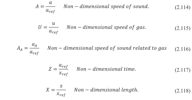
The first 2 lines are linked to the characteristics propagation nature of the wave motion in the ducts, since the terms (u+a) and (u-a) represent the absolute speed of propagation of pressure waves; the third line is instead correlated to the motion of fluid particles, and provides information on the level of entropy in the ducts. An effective graphic representation is shown in fig. 2.3.

The single feature line represents the separation between two regions of the plan, in which the fluid-dynamic properties differ in infinitesimal quantities; they therefore constitute discontinuities for the derived quantities, for example the speed, but not for the fluid. On the three lines, described by eq. 2.95, 2.96 and 2.97, apply relations (see eq. 2.94) that allow you to transform eq. 2.91, 2.92 and 2.93 in the equations to ordinary derivatives, also known as compatibility equations.

(37)

35

Figure 2:3 Tracking of characteristic lines in the (x, t) discretized.

Without introducing any approximation, you can rewrite the system through compatibility equations, or equations to ordinary derivatives:

𝑑𝑝 𝑑𝑡 + 𝜌𝑎 𝑑𝑢 𝑑𝑡 + Δ1+ Δ2+ Δ3 = 0 (2.98) 𝑑𝑝 𝑑𝑡 − 𝜌𝑎 𝑑𝑢 𝑑𝑡 + Δ1+ Δ2− Δ3 = 0 (2.99) 𝑑𝑝 𝑑𝑡− 𝑎 2𝑑𝜌 𝑑𝑡+ Δ1 = 0 (2.100)

To simplify the discussion, it develops the case of isentropic flow in ducts with a constant section. In these conditions, the terms source Δ1, Δ2, Δ3 is cancel and compatibility equations become:

𝑑𝑝 + 𝑝𝑎 ∙ 𝑑𝑢 = 0 (2.101)

𝑑𝑝 − 𝑝𝑎 ∙ 𝑑𝑢 = 0 (2.102)

(38)

36 it is also appropriate to the isentropic transformation relations:

𝑝

𝜌𝑘 = 𝑐𝑜𝑛𝑠𝑡 (2.104)

𝜌 𝑎2⁄𝑘−1

= 𝑐𝑜𝑛𝑠𝑡 _(2.105)

Differentiating 2.106 relationships, 2.105 and placing them in Eq. 2.101, 2.102 is obtained:

𝑑𝑢 + 2

𝑘 − 1𝑑𝑎 = 0 (2.106)

𝑑𝑢 − 2

𝑘 − 1𝑑𝑎 = 0 (2.107)

From these one obtains the differential of the sound velocity compared to the flow velocity, obtaining: 𝑑𝑎 𝑑𝑢= − 𝑘 − 1 2 (2.108) 𝑑𝑎 𝑑𝑢= + 𝑘 − 1 2 (2.109)

The eq. 2.108, 2.109 accompanied of the respective equations of the characteristics lines (eq. 2.95, 2.96) can be represented on the planes (x, t) and (u, a), shown in Fig. 2.4, which are named respectively:

- Location diagram: on which lines features are represented (eq. 2.95, 2.96);

- State diagram: on which the differentials are represented in the speed of sound relative to the flow velocity.

They introduce 2 families of curves to identify the curves associated progressive wave (λ) and those associated with the regressive (β):

(39)

37 𝜆−→ { 𝑑𝑢 𝑑𝑡 = 𝑢 + 𝑎 𝑑𝑎 𝑑𝑢= − 𝑘 − 1 2 𝛽−→ { 𝑑𝑢 𝑑𝑡 = 𝑢 − 𝑎 𝑑𝑎 𝑑𝑢= + 𝑘 − 1 2

Figure 2:4: Position diagram (a) and state (b) for the families of λ and β curves.

The solution can be determined graphically by the intersection of the two families of characteristic curves.

Rewriting eq. 2.108, 2.109 as:

𝑑 (𝑢 + 2

𝑘 − 1𝑎) = 0 ⟶ 𝜆 (2.110)

𝑑 (𝑢 − 2

𝑘 − 1𝑎) = 0 ⟶ 𝛽 (2.111)

we realize that the words in brackets of 2 equations are constant along the characteristic lines and define the Riemann invariants J + and J-.

𝐽₊ = 𝑢 + 2

(40)

38 𝐽− = 𝑢 −

2

𝑘 − 1𝑎 𝑐𝑢𝑡𝑠 𝑑𝑜𝑤𝑛 ⟶ 𝛽 (2.113)

The terms Δ source assume a non-null value, the invariants of Riemann become the Riemann variables and takes the curvature of the lines drawn on the state diagram.

Up to this point it is not any approximation, but they are only manipulated with the initial equations to arrive at a formulation suitable to the resolution through numerical approach. Before going into the actual numerical method, we should define new variables:

𝐴 = 𝑎 𝑎𝑟𝑒𝑓 𝑁𝑜𝑛 − 𝑑𝑖𝑚𝑒𝑛𝑠𝑖𝑜𝑛𝑎𝑙 𝑠𝑝𝑒𝑒𝑑 𝑜𝑓 𝑠𝑜𝑢𝑛𝑑. _(2.114) 𝑈 = 𝑢 𝑎_𝑟𝑒𝑓 𝑁𝑜𝑛 − 𝑑𝑖𝑚𝑒𝑛𝑠𝑖𝑜𝑛𝑎𝑙 𝑠𝑝𝑒𝑒𝑑 𝑜𝑓 𝑔𝑎𝑠. (2.115) 𝐴𝐴 = 𝑎_𝐴 𝑎𝑟𝑒𝑓 𝑁𝑜𝑛 − 𝑑𝑖𝑚𝑒𝑛𝑠𝑖𝑜𝑛𝑎𝑙 𝑠𝑝𝑒𝑒𝑑 𝑜𝑓 𝑠𝑜𝑢𝑛𝑑 𝑟𝑒𝑙𝑎𝑡𝑒𝑑 𝑡𝑜 𝑔𝑎𝑠 _(2.116) 𝑍 =𝑎𝑟𝑒𝑓 𝑥_𝑟𝑒𝑓 𝑁𝑜𝑛 − 𝑑𝑖𝑚𝑒𝑛𝑠𝑖𝑜𝑛𝑎𝑙 𝑡𝑖𝑚𝑒. (2.117) 𝑋 = 𝑥 𝑥_𝑟𝑒𝑓 𝑁𝑜𝑛 − 𝑑𝑖𝑚𝑒𝑛𝑠𝑖𝑜𝑛𝑎𝑙 𝑙𝑒𝑛𝑔𝑡ℎ. (2.118)

where aref, pref, xref are a constant reference values, appropriately chosen for the calculation, whose physical interpretation is instant referring to the following diagram:

Figure 2:5 :a-s diagram on which it is possible to recognize the reference values of: the speed of sound, pressure and entropy.

(41)

39 On the diagram of Fig. 2.5, you can define the speed of aA sound. Starting from the local conditions of p, ρ and hence the speed of sound in, it performs an expansion processing (or compression) isentropic up to the reference pressure pref which corresponds to the speed of sound aA.

The fictitious transformation is isentropic, so you can write the classic relations: 𝑝 𝑝_𝑟𝑒𝑓 = ( 𝑎 𝑎_𝐴) 2𝑘 𝑘−1 _(2.119) 𝜌 𝜌𝐴 = ( 𝑝 𝑝𝑟𝑒𝑓 ) 1 𝑘 (2.120)

In general, for a flow non-isentropic, the value of entropy ‘s’ of the initial state is different from sref therefore aA is distinct from aref isobaric of pref reference. One senses that the aA magnitude is related to the entropy of the AA variable, which represents the entropy level of the gas relative to the reference condition local and especially dynamic gas state, can be immediately related to the entropy variation Δs=s-sref.

Isobaric infinitesimal long increment in entropy gives us:

𝑑𝑠_{𝑝=𝑐𝑜𝑛𝑠𝑡} =𝑑ℎ

𝑇 = 𝑐𝑝 𝑑ℎ

𝑑ℎ (2.121)

knowing that the enthalpy and its infinitesimal variation can be expressed in function of the speed of sound: ℎ = 𝑐_𝑝𝑇 = 𝑘𝑅𝑇 𝑘 − 1= 𝑘 𝑘 − 1∙ 𝑝 𝜌= 𝑎2 𝑘 − 1 (2.122) 𝑑ℎ ℎ = 2𝑑𝑎 𝑎 (2.123)

(42)

40

𝑑𝑠_{𝑝=𝑐𝑜𝑛𝑠𝑡} =𝑑ℎ

𝑇 = 2𝑐𝑝 𝑑𝑎

𝑎 (2.124)

The link between entropy and the speed of sound can be expressed in integral form and dimensionless by:

𝐴_𝐴 = 𝑎𝐴 𝑎_𝑟𝑒𝑓 = 𝑒

(𝑠−𝑠𝑟𝑒𝑓)

2𝑐𝑝 (2.125)

Continuing the discussion, they introduce the Riemann variables as dimensionless calling λ and β: 𝜆 = 𝐴 +𝑘 − 1 2 𝑈 𝑐𝑢𝑡𝑠 𝑑𝑜𝑤𝑛 𝑙𝑖𝑛𝑒 ( 𝑑𝑋 𝑑𝑍)_𝜆 = 𝑈 + 𝐴 (2.126) 𝛽 = 𝐴 −𝑘 − 1 2 𝑈 𝑐𝑢𝑡𝑠 𝑑𝑜𝑤𝑛 𝑙𝑖𝑛𝑒 ( 𝑑𝑋 𝑑𝑍)_𝛽 = 𝑈 − 𝐴 (2.127)

In the presence of isentropic flow, λ and β assume constant values, becoming the invariants of Riemann, while in the opposite case their variation along the characteristic lines is expressed as:

𝑑𝜆 = 𝑑𝐴 +𝑘 − 1

2 𝑑𝑈 (2.128)

𝑑𝛽 = 𝑑𝐴 −𝑘 − 1

2 𝑑𝑈 (2.129)

The quantities dλ and dβ are determined by the compatibility equations (eq.2.101-102-103), in dimensionless form and rearranged, and the direction of equations.

Following solved equations are applied to the three characteristics families: - λ Characteristic (traveling wave)

Equation direction:

(𝑑𝑋

(43)

41 Compatibility Equation: 𝑑𝜆 = −(𝑘 − 1) ∙ (𝐴𝑈) 2 ∙ ( 1 𝐹 𝑑𝑓 𝑑𝑋) 𝑑𝑍 −(𝑘 − 1) 2 2𝑥_𝑟𝑒𝑓𝑓 𝐷 𝑈 2 𝑈 |𝑈|[1 − (𝑘 − 1) 𝑈 𝐴] 𝑑𝑍 +(𝑘 − 1) 2 2 𝑞̇𝑥_𝑟𝑒𝑓 𝑎_𝑟𝑒𝑓3 1 𝐴𝑑𝑍 + 𝐴 𝐴_𝐴𝑑𝐴𝐴 (2.131)

-  Characteristic (regressive wave) Equation direction: (𝑑𝑋 𝑑𝑍)𝛽 = 𝑈 − 𝐴 (2.132) Compatibility Equation: 𝑑𝛽 = −(𝑘 − 1) ∙ (𝐴𝑈) 2 ∙ ( 1 𝐹 𝑑𝑓 𝑑𝑋) 𝑑𝑍 +(𝑘 − 1) 2 2𝑥𝑟𝑒𝑓𝑓 𝐷 𝑈 2 𝑈 |𝑈|[1 − (𝑘 − 1) 𝑈 𝐴] 𝑑𝑍 +(𝑘 − 1) 2 2 𝑞̇𝑥_𝑟𝑒𝑓 𝑎_𝑟𝑒𝑓3 1 𝐴𝑑𝑍 + 𝐴 𝐴_𝐴𝑑𝐴𝐴 (2.133)

- Trajectory Feature (flow line or path line) Equation direction: (𝑑𝑋 𝑑𝑍) = 𝑈 (2.134) Compatibility Equation: 𝑑𝐴𝐴 = (𝑘 − 1) 2 𝐴_𝐴 𝐴2( 2𝑥𝑟𝑒𝑓𝑓 𝐷 |𝑈 3_{| +}𝑞̇𝑥𝑟𝑒𝑓 𝑎_𝑟𝑒𝑓3 ) 𝑑𝑍 (2.135)

(44)

42 In the first two compatibility equations (eq. 2.131-2.133) it is observed that changes in variables Riemann, dλ and dβ, depend on four basic terms due respectively to the change of section of the pipe, friction, heat exchange and the entropy change.

𝑑(𝜆, 𝛽) = 𝛿_{𝑠𝑒𝑐𝑡𝑖𝑜𝑛}+ 𝛿_{𝑓𝑟𝑖𝑐𝑡𝑖𝑜𝑛} + 𝛿_{ℎ𝑒𝑎𝑡} + 𝛿_{𝑒𝑛𝑡𝑟𝑜𝑝𝑦} (2.136)

In the third equation of compatibility, the increase of entropy level depends only from the contributions due to friction and heat exchanges.

𝑑𝐴_𝐴 = 𝛿_{𝑓𝑟𝑖𝑐𝑡𝑖𝑜𝑛}+ 𝛿_{ℎ𝑒𝑎𝑡} (2.137)

Now consider the physical features of the Method of Characteristics.

In a compressible and unsteady flow, the conditions, in a given section are determined by the mass transport rate and the pressure perturbations that propagate at the speed of sound through the fluid itself. As shown in fig. 2.6, in a generic section of the pipe at time t+t P of the flow conditions can be influenced only by the states of the gas relative to the previous time t, i.e the points C, D and F. The lines connecting the points P to C, D and F represent characteristic lines in the plane (x,t) and their inclination depends on the absolute speed of sound of the gas in this point

(45)

43 Operationally, we proceed in the following way: notes the Riemann variables at time Z, is the change in entropy through the equation of the flow line 2.135, and then the variations along the lines of the characteristics of Riemann variables through the 2.131 compatibility equations and 2.133. It is thus possible to determine the new value of the Riemann variables at time Z + ΔZ in the following way:

𝜆𝑍+Δ𝑍 = 𝜆 + Δ𝜆 _(2.138)

𝛽_𝑍+Δ𝑍 = 𝛽 + Δ𝑑 (2.139)

At this point the solution is determined through deriving from the relations eq 2.126 and 2.127:

𝐴 =𝜆 + 𝛽

2 (2.140)

𝑈 =𝜆 − 𝛽

𝑘 − 1 (2.141)

Is now introduced to the Method of Characteristics to mesh, namely it adopts a numerical method for the estimation of the analytical solution.

In the Method of Characteristics to mesh, belonging to the family of explicit methods, the points of intersection of the characteristic lines have a known position and defined in the (x, t). To discretize the space-time domain using a rectangular grid computing with the following features:

SPACE: discretization along the x coordinate is fixed according to the number of mesh, or sub-elements, with which the duct is divided. For a number of the sub-elements correspond l+1 compute nodes. Increasing computing nodes, thereby reducing the size of the mesh, you will get more accurate results.

TIME: the size of the time step is determined based on the condition of stability dictated by the policy CFL (Courant-Friedrichs-Lewy). Considering the finite propagation velocity of a wave of pressure in a conduit such as the speed of sound in added to the flow velocity u, the distance traveled by the wave in the time of Dt calculation step must be less than the size of the mesh Δx. It therefore introduces the CFL number:

(46)

44

𝐶𝐹𝐿 = (𝑎 + |𝑢|)Δ𝑡

Δ𝑥 ≤ 1 (2.142)

𝐶𝐹𝐿 = (𝐴 + |𝑈|)Δ𝑍

Δ𝑋 ≤ 1 (2.143)

In order for all the nodes belonging to the grid at the time Z+ΔZ from falling into the domain of influence the CFL has to assume values ≤ 1.

The calculation of the Riemann variables and tracking features lines are made only in the grid nodes at each time step, as shown in the following figure:

Figure 2:7 Grid space-time used for the calculation of the Riemann variables with the method of characteristics

Now rename the Riemann variables as: λI corresponding to λ and λII corresponding to β; this allows a generalization that simplifies the calculation procedure.

Note the values of the three variables λI, λII, AA in each mesh point of the duct at the dimensionless time Z, it determines the time step ΔZ, according to the criterion of the CFL so as to define the calculation grid at time Z + ΔZ. For the tracking characteristics of the lines to the new time step we proceed back in time, ie the two families of λI and λII lines are drawn from each node of the mesh at the time Z + ΔZ, as shown in fig. 2.8.

(47)

45

Figure 2:8 Tracking feature lines back in time, starting from the node s in Z+ΔZ (point R') up to the P points to the time Z.

The two characteristic lines intersect the abscissa axis at the time Z in two points L and R, distinct from the nodes. The slope of the lines is held constant but in reality, they are curved and then introduces an approximation. The smaller is the size of the calculation grid and the lower the numerical error associated with this approximation. In addition to the characteristics lines it is also track the flow line that intersects the axis of the space at the point S.

It is shown that the position of the points L and R on the mesh (Fig. 2.8) can be calculated from the known values of λI and λII in adjacent nodes, for brevity it will only show the calculation of the position of the point L, as regard R is completely analogous process.

λI being the progressive characteristic curve, the following relationship: 𝛿𝑋_𝐿

Δ𝑍 = 𝑈𝐿+ 𝐴𝐿 (2.144)

Using eq. 2.140 and 2.141 and drifting the 2.144 you get: 𝛿𝑋𝐿

Δ𝑍 = 𝑎𝜆𝐼𝐿 + 𝑏𝜆𝐼𝐼𝐿 (2.145)

where a, b represents two constants dependent on the nature of the gas: 𝑎 = 𝑘 + 1

(48)

46 𝑏 = 3 − 𝑘

2(𝑘 − 1) (2.147)

- λI the point L is determined by linear interpolation between the known values of the same magnitude in the i and i-1 nodes:

𝜆_𝐼_𝐿 = 𝜆_𝐼_𝑖−𝛿𝑋𝐿

Δ𝑋 (𝜆𝐼𝑖− 𝜆𝐼𝑖−1) (2.148)

- λII at the point L it is determined in a similar manner to λ: 𝜆_𝐼𝐼_𝐿 = 𝜆_𝐼𝐼_𝑖 −𝛿𝑋𝐿

Δ𝑋 (𝜆𝐼𝐼𝑖− 𝜆𝐼𝐼𝑖−1) (2.149)

Replacing the 2.148 and the 2.149 in 2.145 is finally obtained: 𝛿𝑋_𝐿 Δ𝑋 = 𝑎𝜆_𝐼_𝑖+ 𝑏𝜆_𝐼𝐼_𝑖 Δ𝑋 Δ𝑍 + 𝑎(𝜆𝐼𝑖− 𝜆𝐼𝑖−1) − 𝑏(𝜆𝐼𝐼𝑖− 𝜆𝐼𝐼𝑖−1) (2.150)

At this point the values of the variables are known Riemann and in general all the other quantities in the characteristics of line intersections points with the abscissa axis at the time Z; before you can evaluate Δ1 and Δ2 is necessary to calculate the entropy change along the same characteristics.

To do this it uses the equation of the flow line compatibility (2.135) in which the magnitude, AA, U, q and f must be calculated in the point S to means of a linear interpolation of the neighboring nodes:

𝐺_𝑠 = 𝐺_𝑖 −𝛿𝑋𝑠

Δ𝑋 (𝐺𝑖 − 𝐺𝑖−1) (2.151)

Where G indicates a generic observable and 𝛿𝑋_𝑠 Δ𝑋 = 𝜆_𝐼_𝑖− 𝜆_𝐼𝐼_𝑖 Δ𝑋 Δ𝑍 (𝑘 + 1) + (𝜆𝐼𝑖− 𝜆𝐼𝑖−1) − (𝜆𝐼𝐼𝑖− 𝜆𝐼𝐼𝑖−1) (2.152)

(49)

47 Now it is known the value of AAS and dAAS from which it is possible to calculate the entropy of the point P (AAP) through the equation:

𝐴_𝐴_𝑃 = 𝐴_𝐴_𝑆+ 𝑑𝐴_𝐴_𝑆 (2.153)

Known AAP for finding the entropy change along λI character line and in a similar manner along λII, it will be enough to calculate:

𝑑𝐴_𝐴_𝐿 = 𝐴_𝐴_𝑝+ 𝐴_𝐴_𝐿 (2.154)

dAAL and d AAR, are to be inserted respectively in 2.131 and 2.133 to find  and .

The described numerical method is used to determine the three λI variables, λII, and AA in all the mesh nodes, except the first and last. In fact, starting from the end nodes we can trace back in time only one of the two characteristic lines because the other falls outside of the duct, in the region bordering contour, as shown in fig. 2.7. It suggests that in the node 1 is possible to know λ’Il, directly only while the node I + 1 is possible to know λ’I, because both fall within the duct considered; These two variables are called λin.

To assess the missing Riemann variable, called λout, recourse is to the boundary conditions, it conditions that translate the presence of the environment or of a neighboring component with the end of the duct considered. For the modeling of the boundary conditions it is assumed the hypothesis of almost stationarity of the phenomena that take place in the boundary regions, or that is, it is supposed that the gas dynamic processes in these regions can be described by a succession of stationary states, spaced by time intervals ΔZ. These assumptions lead to expressing the boundary conditions as algebraic equations arising from the conservation equations for steady flow and one-dimensional, unsteady neglecting the terms of type t. Numerous situations to the contour can be described with this approach, including: open ends in a constant pressure environment, end partially open, junctions of two ducts with abrupt variation of section, more ducts junctions and others.

In conclusion, please note that, by adopting a linear interpolation technique in the space of the grid, the gate of the Features method to be accurate to the first order in space and time. This characteristic turns out to be a limitation in the very detailed analysis, since they can not be picked by small oscillations of the magnitudes at high frequencies.

(50)

48

2.2. Shock-Capturing methods:

The results of fluid dynamic simulations can be greatly improved by using, for the resolution of hyperbolic system, more robust and accurate than the method of numerical methods to mesh Features. The fundamental merit of the Shock-Capturing methods resides in the ability to grasp correctly any discontinuities in the solution, as for example: shock waves, contact discontinuities due to temperature or chemical composition. Within this family, the methods to the symmetrical finite differences have proved the most efficient, representing a good compromise between: accuracy, the goodness of the solution, simplicity and calculation times. The symmetry of the method consists in applying in each node of the grid the same scheme with finite differences for expressing the terms of the spatial derivatives, irrespective of the flow field characteristics.

The methods described below are explicit and have an accuracy of the II order in the space-time domain. Unfortunately, as is known from the theorem of Godunov, the fact of having an accuracy of higher order at the first port to have problems of spurious oscillations in the solution found, and then is indispensable the use of special algorithms accessories to mitigate this phenomenon.

As described in chapter 1, the Shock-Capturing methods are applied to the hyperbolic system written in conservative form and matrix, complete additional hypothesis on the evolving gas model. Referring to Eq. 1.34 and clearing of the source terms vectors, we obtain the Euler equations describing the isentropic flow in a duct with constant cross section:

𝜕𝑊̅ (𝑥, 𝑡)

𝜕𝑡 +

𝜕𝐹̅(𝑊̅ )

𝜕𝑥 = 0 (2.155)

By integrating Eq.2.155 in space x and in time t and applying the divergence theorem of Gauss, we obtained: ∫ ∫ (𝜕𝑊̅ 𝜕𝑡 + 𝜕𝐹̅ 𝜕𝑥) 𝑑𝑥 ∙ 𝑑𝑡 = 0 𝑥+Δ𝑥 𝑥 𝑡+Δ𝑡 𝑡 (2.156)

The use of finite difference methods for the solution of eq. 2.156 requires the discretization of the space-time domain through mesh subdivision. The carrier, allows to fully characterize the motion of the flow and can be approximated by the following relationship: