A mathematical model for migraine aura

(1)

Alma Mater Studiorum · Università di Bologna

SCUOLA DI SCIENZE Corso di Laurea in Matematica

A MATHEMATICAL MODEL FOR MIGRAINE AURA

Tesi di Laurea in Analisi Matematica

Relatore:

Chiar.ma Prof.ssa

GIOVANNA CITTI

Presentata da:

CHIARA

DI DOMENICO

Sessione di Dicembre

Anno Accademico 2015/2016

(2)

(3)

(4)

(5)

Beauty of whatever kind, in its supreme development, invariably excites the sensitive soul to tears.

(Edgar Allan Poe)

(6)

(7)

Introduction

Migraine is a chronic neurological disease characterized by episodic headaches, of moderate to severe intensity, pulsing character and unilateral localization.

The attack is often preceded by an aura, that is a set of neurological symptoms, mainly sensory hallucinations.

Here we will focus on the classic visual aura, which typically begins in a small area of the visual field as a spot with indistinct boundary, called "scotoma" (Fig.(a)).

The scotoma gradually expands assuming the shape of a crescent or a C (Fig.(b)). While advancing, on one of its two edges appear, zigzag, lines and geometric shapes bright and sparkling and for this reason it is often called "fortification pattern".

(a) Right-sided fortification. The sco-toma enclosed by the scintillating zigzag pattern is indicated by a perceptual filling-in based on the visual surround. [Image taken from "A computational perspective on migraine aura"]

(b) Successive sketches of a scintillating sco-toma, the so-called fortification. The crosses indicate the center of gaze, and the numbers state the time in minutes that passed for each fortification pattern since its first appearance close to the center of gaze.

[Image taken from "Migraine aura dynamics after reverse retinotopic mapping of weak ex-citation waves in the primary visual cortex"]

The visual aura seems to reflect a fundamental organizational principle of the cerebral cortex, namely its ability to map topographically sensory input. Therefore, the scotoma

(8)

no-invasive imaging techniques.

In Chapter 1 we will describe, from a neural point of view, the scotoma and the mecha-nism that is at the base of its formation and propagation.

In Chapter 2 we will describe the map from the retina to the cortex, called "retino-cortical map", which performs a deformation of the visual stimuli and models them via a complex logarithm

w = ln(z),

where w represents a point in the cortical plane and z represents a point in the visual field.

We will see that under the action of this map the wave front described in the Figure (b) appears more straight allowing a simpler modellization.

In Chapter 3 we provide a macroscopical description of the scotoma’s propagation, for-getting its fortification pattern. This propagation phenomenon, known as "Cortical Spreading Depression" (CSD), will be described as the motion by curvature of an open curve with free ends.

We will show that the evolution of the wave front is modeled by an equation of type: ∂k ∂t + ∂k ∂l( Z l 0 kV dξ + G) = V k2+ ∂ 2_k ∂l2,

where l is the arc length of the curve, k = k(l, t) is the curvature as a function of the arc length l and of the time t, V is the normal velocity at each point of the front and G is the tangential velocity at the free ends.

In Chapter 4 we will justify the fortification pattern via the propagation of the wave front in the pinwheels structure of the primary visual cortex, which is the structure re-sponsible for orientation detection. It can be modeled as a fiber bundle over the 2D retinal plane R, with total space R × P1 and projection π : R × P1 → R.

In Chapter 5 we conclude the model of migraine aura showing as all the aspects de-scribed previously provide an unitary description of the phenomenon.

(9)

Introduzione

L’emicrania è un disturbo neurologico cronico caratterizzato da episodici mal di testa, di intensità da moderata a severa, a carattere pulsante e a localizzazione unilaterale. L’attacco è frequentemente preceduto da un’aura, cioè un insieme di sintomi di tipo neu-rologico, principalmente allucinazioni sensoriali.

Qui ci concentriamo sulla classica aura visiva, che tipicamente comincia in una piccola area del campo visivo e si presenta come una macchia dai bordi indistinti, chiamata "sco-toma" (Fig.(c)).

Lo scotoma si espande gradualmente assumendo la forma di una falce o di una C (Fig.(d)).

(c) Fortificazione del lato destro. Lo scotoma delimitato dallo schema a zigzag scintillante è caratterizzato da un completamento percettivo basato sulla scena visiva circostante.

[Immagine presa da "A computational perspective on migraine aura"]

(d) Schizzi successivi dello scotoma scintil-lante, il cosiddetto schema di fortificazione. Le croci indicano il centro dello sguardo e i numeri rappresentano il tempo in minuti trascorso dalla prima apparizione dello sco-toma vicino al centro dello sguardo.

[Immagine presa da "Migraine aura dynamics after reverse retinotopic mapping of weak ex-citation waves in the primary visual cortex"]

Mentre avanza, su uno dei suoi due bordi appaiono, a zigzag, linee e forme geometriche luminose e scintillanti e per questa ragione esso è spesso chiamato "schema di fortifi-cazione".

(10)

questa ragione, lo scotoma fa luce sugli schemi spazio-temporali corticali, e permette la rappresentazione dell’organizzazione funzionale della corteccia con una precisione non ancora raggiungibile dalle attuali tecniche di imaging di tipo non invasivo.

Nel Capitolo 1 descriveremo, da un punto di vista neurale, lo scotoma e il meccanismo che è la base della sua formazione e propagazione.

Nel Capitolo 2 descriveremo la mappa dalla retina alla corteccia, chiamata "mappa retino-corticale", che esegue una deformazione degli stimoli visivi e li modella tramite un logaritmo complesso

w = ln(z),

dove w rappresenta un punto nel piano corticale e z rappresenta un punto nel campo visivo.

Nel Capitolo 3 daremo una descrizione macroscopica della propagazione dello scotoma, dimenticando il suo schema di fortificazione. Il fenomeno di propagazione, noto come "Cortical Spreading Depression" (CSD), sarà descritto come il moto per curvatura di una curva aperta con estremità libere.

Mostreremo che l’evoluzione del fronte d’onda è modellata da un’equazione del tipo: ∂k ∂t + ∂k ∂l( Z l 0 kV dξ + G) = V k2+ ∂ 2_k ∂l2,

dove l è la lunghezza d’arco della curva, k=k(l,t) è la curvatura in funzione della lunghezza d’arco l e del tempo t, V è la velocità normale a ogni punto del fronte e G è la velocità tangente alle estremità libere.

Nel Capitolo 4 giustificheremo lo schema di fortificazione attraverso la propagazione del fronte d’onda nella struttura a pinwheels della corteccia visiva primaria, che è la struttura responsabile del rilevamento dell’orientazione. Quest’ultima può essere modellata con un fibrato sul piano retinico 2D (R), con spazio totale R × P1 e proiezione π : R × P1 → R. Nel Capitolo 5 concluderemo il modello dell’aura emicranica mostrando come gli aspetti precedentemente descritti forniscano una descrizione unitaria del fenomeno.

(11)

Chapter 1 The neural basis of Migraine Aura

The term "scotoma" indicates, in medical language,

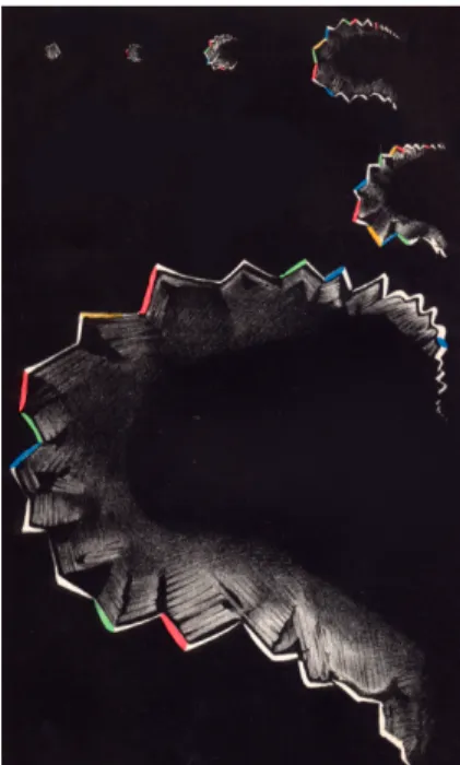
Figure 1.1: Artistic representa-tions, very similar to the real-ity, that show the different expan-sion’s stages of the fortification pattern.

a complete or partial blind area, inside the visual field. The scintillating scotoma (Fig.1.1) is a special type of scotoma which represents the prodromal symptom of migraine, a chronic neurological disease characterized by episodic headaches, from moderate to severe inten-sity, pulsing character and unilateral localization. It is manifested by the appearance, in the visual field, of an arch of flashing light, formed by the connection of various broken lines of different colors (yellow, red, blue, green).

This arch is the border of an area with a reduced or absent response to light stimulus, which corresponds to an area with reduced or absent sensitivity of the retina.

The disturbance lasts for few minutes, typically not more than half an hour, then disappears, leaving no visual trace.

(14)

1.1 Eye

The eye is the sensory organ that let us able to see, by turning the light that hits it in informations that, in the form of electrical impulses, go to the brain.

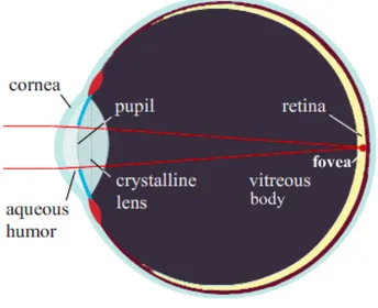
When we stare at an object, the light who comes from it enters our eyes crosses a se-ries of natural lenses, which are, in sequence, the cornea, the crystalline and the vitreous body, and will "impress" the retina (Fig.1.2). The latter, excited by the light that strikes it, transmits informations to the brain, sending electrical impulses through a biological cable: the optic nerve.

Figure 1.2: Eye’s anatomy.

In this study we will focus on the retina. It is divided into two areas: a central area, circular with the center in the fovea, rich in cones (nerve cells in charge of the perception and recognition of colors and distinct vision), and a peripheral one, where, on the other hand, rods prevail (other photoreceptors which allow the vision in low light).

The retina remains in its natural place thanks to the pressure of the vitreous body, the gelatinous liquid that fills the eyeball.

When a light stimulus enters the eye and affects the retina, the rods and cones are ac-tivated: they capture the light and transform it into electrical impulses that are then transmitted, with the collaboration of others important retinal nerve cells, to the fibers of the optic nerve.

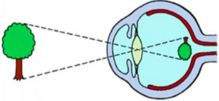
As it is well known, focusing on the retina produces an inverted image: the light that comes from above is focused on the lower part of the retina, close to the cheekbones, while the light coming from the bottom is focused on the upper part of the retina, near the eyebrows (Fig.1.3).

(15)

1.1 Eye 3

Figure 1.3: Projection of an object on the retina.

1.1.1 Visual field

The visual field is the portion of space perceived by the eyes when your gaze is fixed on a point (fixation point) (Fig.1.4). The fixation point is what is projected, in the retina, on the fovea.

Figure 1.4: Visual field. On the right: the central yellow part is the area where you are able to perceive the details, the sides in gray represent the peripheral visual areas, i.e. those in which you cannot make out the details.

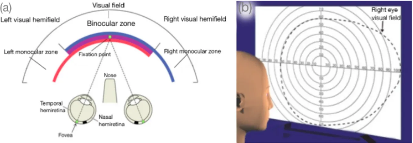
The visual field is divided into two hemifields: the right hemifield and the left one. Moreover we can distinguish: binocular visual area (area of the field in which the visual field of the right eye and the one of the left eye intersect); right monocular visual area (the right eye visual field area which is not intersecting the left visual field); left monoc-ular visual area (Fig.1.5(a)).

In many contexts, for simplicity, the visual field, object of three-dimensional nature, is made two-dimensional: as in a photography, the portion of the space perceived by the eye is projected on a plane (Fig.1.5(b)). On this plane concentric circles fraction the

(16)

image: each circle corresponding to a value of retinal eccentricity, which is the measure-ment of the radial distance from the fovea.

Figure 1.5: (a): Visual field areas. The center axis of the eye (dashed line in the figure) divides the retina into two halves: the nasal hemiretina and the temporal hemiretina. (b): Two-dimensional version of the visual field. The numbers on the orthogonal axes represent the retinal eccentricity.

(17)

1.2 Brain 5

1.2 Brain

1.2.1 Optic nerve

The optic nerve is the nerve which conveys visual informations from the retina to the brain. It leaves the eye socket through the optic canal, reaching the optic chiasm, in which we can observe a partial decussation of the nerve fibers (crossing): those coming from the nasal hemiretina cross and continue in the contralateral optic tract.

Most of the optical fibre nerves end in lateral geniculate bodies, from where the visual information is transmitted to the primary visual cortex (see section 1.2.2). The remainder ends in the midbrain.

In the lateral geniculate body "internal representations" of the space that is visible around us are created: the left visual hemifield is represented in the right hemisphere, the right one in the left hemisphere (Fig.1.6).

Figure 1.6: Path of the optic nerve from the retina to the visual cortex and cortical represen-tation of the visual field.

(18)

1.2.2 Primary visual cortex (V1)

The term "primary visual cortex" refers to a part of the cerebral cortex, located in the occipital lobe, where the development of visual images takes place (Fig.1.7).

Figure 1.7: In yellow the primary visual cortex.

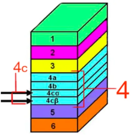
The primary visual cortex is composed of 6 horizontal layers (Fig.1.8). The most inter-esting part for us is the layer 4 and, in particular, its sublayer 4c, where most of the fibers coming from the lateral geniculate body are attached.

Figure 1.8: The six layers of the primary visual cortex. Marked in red layer 4 and its sublayer 4c, split up into the layers 4cα and 4cβ.

Over the last forty years, there have been several experimental studies to explain the functional organization of the visual cortex.

(19)

1.2 Brain 7

Experiments consist in measuring the neuronal activity with one or more microelec-trodes, while these penetrate V1 in a perpendicular direction or nearly tangential to it. Hubel and Wiesel, first, discovered an orderly organization in the visual cortex.

According to what was observed, if one penetrates the cortex in a perpendicular direc-tion, two types of cells can be found, called simple and complex cells, joined by the same retinal location of the receptive field (domain of the retina to which the cell is connected through the synapses of the retino-geniculo-cortical path and whose stimulation elicits a peak response) and by the same given orientation stimulus; following an oblique pene-tration (nearly horizontal) sequential changes of the orientation can be noted (10 degrees of orientation between adjacent columns).

This finding led Hubel and Wiesel to interpret the primary visual cortex as a periodic organization of functional units, called columns, containing neurons that encode a par-ticular orientation.

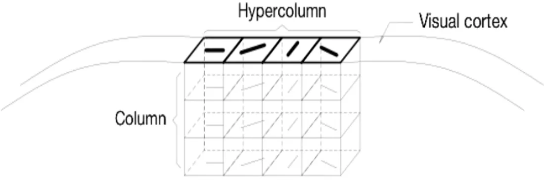
The set of vertical columns corresponding to a complete sequence of orientations (a pe-riod), according to the terminology adopted by Hubel and Wiesel, is called hypercolumn. The hypercolumn, therefore, represents one of the fundamental building blocks of the cortex (Fig.1.9).

Figure 1.9: Functional organization of the primary visual cortex, according to the model of Hubel and Wiesel.

It is important to emphasize the fact that a column accesses at region of the visual field that corresponds to the set of all the receptive fields of the cells contained therein. Furthermore, this region is largely shared by the nearby columns. More precisely, it is necessary that you move around in the cortex about 2.4 mm [Albus 1975], or about two hypercolumns, for have that two columns access at completely distinct region of the image in the visual field.

We observe, lastly, that the primary visual cortex is retinotopic, i.e. it reproduces the retina’s topography.

(20)

1.3 Cortical Spreading Depression (CSD)

The neuropathophysiological phenomenon that causes migraine aura is the so-called "Cortical Spreading Depression" (CSD), that is a wave of depolarization of a large num-ber of neurons of the cerebral cortex.

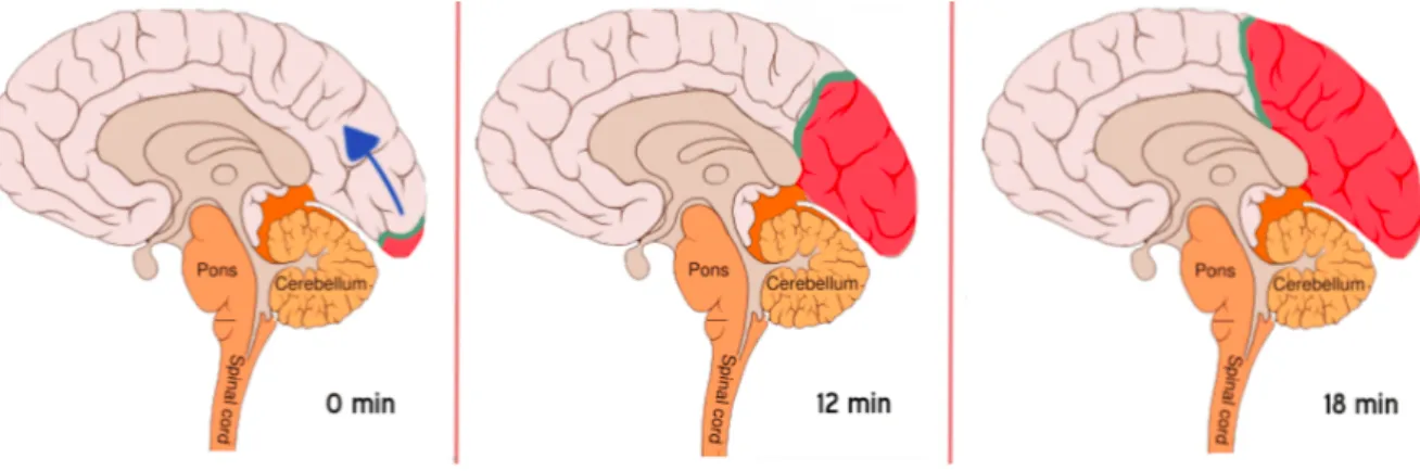
It often arises in V1 and spreads slowly (3 mm/min) through the cortex, generating neuronal excitation in the wave front, followed, then, by cortical depression (Fig.1.10). The excitement causes a positive neurological symptom (the zig zag pattern), the de-pression causes the negative neurological symptom (scotoma).

Studies show that the advancement of the scotoma in the visual field goes hand in hand with the advancing wave of depolarization in the cerebral cortex.

Figure 1.10: Evolution of the CSD. The green area represents the wave front (excitatory), the red one the cortical depression. The shape of the wave, and thus of its front, can vary from attack to attack and from patient to patient.

1.3.1 CSD as a trigger-wave

By "excitable media" we intend those dynamic systems in which a pulse travels be-cause the elements of the system are affected by the state of the neighborhood: if those nearby are excited, elements of the system go from a state of quiescence to a state of excitement, after which they enter into a recovery state which prepares them for the next possible excitement.

Therefore, the elements of a system like this can be only in one of the following states: quiescent, that is available for excitation; excited; refractory to excitation.

The rule is that each element remains quiescent until it is excited by one near it; at that point, the element enters into a state of excitation and, immediately after, in that of refractoriness, where it remains for a certain time.

(21)

1.3 Cortical Spreading Depression (CSD) 9

The cerebral cortex is an excitable medium.

When an element of an excitable medium produces an explosion of activity, an exci-tation wave may be generated: the local exciexci-tation triggers, usually due to diffusion, excitement in its surroundings. A wave of this type is called trigger-wave and is very frequent in excitable media.

The CSD is a trigger-wave.

In migraine sufferers the visual cortex is functionally hyperexcitable. In response to psychological or physiological stress, or a combination of these, the inhibition function of the cortex fails: extracellular potassium is accumulated, electrical gradient is generated, therefore a potential action, and so the CSD is triggered.

(22)

(23)

Chapter 2 The retino-cortical map and the

distortion of the scotoma

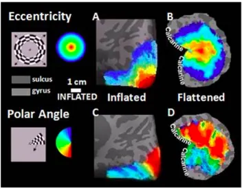
In this chapter we will recall a model for the retino-cortical map (or retinotopic). This is a map induced by the cortical receptors, which describes the mathematical pro-jection of the retina to the primary visual cortex. We will see that it preserves the topology of the visual inputs, but it introduces a geometric deformation (Fig.2.1), which can be modelled as a complex logarithm.

Figure 2.1: Retinotopic maps created by using CBF signal presented on the inflated and flattened brain surface for polar and eccentricity stimuli from the right hemisphere of a representative subject.

[Image taken from http://www.kyb.tuebingen.mpg.de/nc/employee/details/mustafa.html]

(24)

reti-nal plane the curved shape depicted in the Figure (b) (see Introduction), is projected in the cortex to a new wave front, whose shape is its deformed image throught the complex logarithm.

(25)

2.1 The retino-cortical map 13

2.1 The retino-cortical map

The notion of retinotopic map can be traced back to the pioneering anatomical re-search of Polyak (1957), who first suggested the existence of a mathematical projection of the retina to the primary visual cortex. We will study, for simplicity, the construction of the retinotopic map relating to one hemifield.

To describe this projection is necessary to clarify, first of all, what is meant by "cortical magnification factor".

The term "cortical magnification factor" refers, in neurophysiology, to the fact that the number of neurons of the primary visual cortex responsible for processing of a visual stimulus of a given dimension, varies as a function of the position of the stimulus in the visual field: the stimuli located in the center of the visual field, thus in a neighborhood of the fovea, are processed by a large number of neurons, which manage only a small central region of the visual field; conversely, the stimuli localized in the periphery of the visual field are processed by a fewer number of neurons of the primary visual cortex. This concept is very intuitive: when we look at a landscape, a painting, our image in the mirror, what we see better, that is, what we can see in a sharper and more defined way, is what is close to the fixation point, i.e. greater definition means more processing and "a greater number of neurons" means "a higher cortical surface".

So, what happens is that, unlike the peripheral area, the central area of the visual field is enlarged (to its real size) on the cortical surface.

Daniel and Whitteridge defined the cortical magnification factor as the distance trav-elled (in millimeters) on the cortical surface when one point stimulation is moved of one degree, in terms of eccentricity, in the visual field. So, the cortical magnification factor depends on retinal eccentricity, i.e. the radial distance of the stimulus from the fovea. Daniel and Whitteridge have given a precise expression of it:

M (r) = 6

r0.9, (2.1)

where r is, indeed, the retinal eccentricity in degrees.

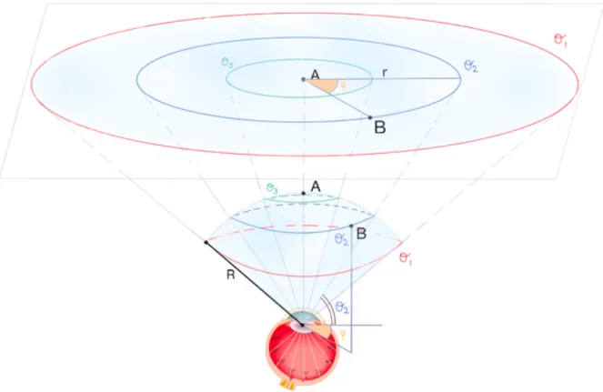
The choice of r as the variable that represents the eccentricity is done with a precise purpose: simplify the "geometry of vision" approximating the visual sphere with its tan-gent plane (Fig.2.2).

The spherical coordinates of eccentricity and azimuth can be approximated by the polar coordinates (r, ϕ) of the plane tangent to it.

In particular, the polar coordinate ϕ is identical to the spherical coordinate describing the azimuth, the polar coordinate r is approximately proportional to the eccentricity, in that, if α is the eccentricity of a certain point on the retina, and R is the radial distance

(26)

of the tangent plane from the retina, we have that

r = Rsinα ≈ Rα. (2.2)

The approximation (2.2) is accurate to 98% for the 20 central degrees of the visual field. For the central foveal representation (less than 1 degree of eccentricity), no magnification data is available. It is assumed that the inverse dependence from eccentricity is tapering gradually to this more central part of the visual field.

The analysis of Daniel and Whitteridge data, expressed by (2.1), can be simplified with the approximation

m = k

r, (2.3)

where k is a constant, r is the retinal eccentricity and m is the cortical magnification factor.

The cortical magnification factor is, actually, a differential quantity: small changes of cor-tical position are correlated to small changes of position in the visual field and conversely. As we are interested in the analytical form of retinotopic map, and not to that of its derivative, we have to find a function (analytic) whose derivative is radially symmetric and is proportional to 1_r.

The analytic function who has this property is the complex logarithm w = kln(z),

where w represents a point in the cortical plane and z = reiϕ represents a point in the visual field.

To make sure the complex logarithm is actually the right analytic function to be consid-ered, we have to observe that the cortical magnification factor of the retinotopic map f at a point z0 can be mathematically written as

m(z0) = lim z→z0 f (z) − f (z0) z − z0 = |f0(z0)| , (2.4)

considering that it is just the amount of which an infinitesimal segment is stretched from the map f (z).

(27)

2.1 The retino-cortical map 15

Figure 2.2: Approximation of the visual sphere (concerning one eye) with its tangent plane that, for clarity of the picture, is represented slightly translated. A is the contact point between the sphere and the plane, ϕ is the azimuth, R is the radius of the sphere, θ is the latitude and r is the radial polar coordinate of the plane tangent to the sphere.

Substituting f (z) = kln(z) in (2.4) one has |f0(z0)| = k z0 = |k| e−iϕ r0 = |k||e −iϕ_| |r0| = k r0 ,

which is precisely the cortical magnification factor experimentally obtained by Daniel and Whitteridge.

(28)

2.2 The induced geometric distortion

To figure out the geometry of the retino-cortical map is necessary to understand the geometry of the complex logarithm and that of its derivative. In this section we will exactly deal with this.

Definition 2.2.1 (Local diffeomorphism). Let us to consider Ω ⊆ Rn an open set and ϕ : Ω → Rn a C∞ map. We call with Dϕx the Jacobian matrix of ϕ calculated in x ∈ Ω.

We say that ϕ is a local diffeomorphism if ∀x ∈ Ω we have that detDϕx 6= 0.

Definition 2.2.2 (Local positive diffeomorphism). We say that ϕ (as we have already said) is a local positive diffeomorphism (or that ϕ preserves the orientation) if ∀x ∈ Ω we have that detDϕx > 0.

Definition 2.2.3 (Conformal map). A map ϕ : Ω → R2 is said conformal if: • ϕ is a local positive diffeomorphism;

• ϕ preserves the angles.

Theorem 2.2.1. A holomorphic function f : Ω → C such that f0(z) 6= 0 ∀z ∈ Ω is conformal.

Proof.

The fact that f is a positive local diffeomorphism if f0 6= 0, came from the fact that for an holomorphic function one has always to apply:

det(Dfz) = |f0(z)| 2

.

Now we will prove that f preserves angles. Let γ : (−1, 1) → Ω be a curve such that γ(0) = z and let ∂γ_∂t(0) = v be the tangent vector to γ in z. We assume that v 6= 0. If v is the tangent vector to the image curve f ◦ γ in f (z), one calculates that

v = ∂

∂tf (γ(t))|t=0= f

0

(z)v.

By hypothesis f0(z) 6= 0, then we can write f0(z) = R(z)eiϕ(z)_{, with R(z) 6= 0.}

Being v = %eiθ_{, we have that}

v = R(z)eiϕ(z)%eiθ = R(z)%ei(ϕ(z)+θ),

i.e. that v is obtained by lengthening or shortening v of an R(z) factor and then rotating it of an angle ϕ(z).

(29)

2.2 The induced geometric distortion 17

γ through for z. Then, if we consider two curves γ1 and γ2 loops z with tangent vectors

in z, respectively, the vectors v1 and v2, we have that the corresponding tangent vectors

to the image curves v1 e v2 differ from v1 and v2 by the same angle ϕ(z). It follows

that, if v1 e v2 form an angle α between them, v1 and v2 form between them the same

angle.

Observation 2.2.1. The complex logarithm is a conformal map.

Definition 2.2.4 (Möbius transformations). Let T be a function of type T (z) = az + b

cz + d , (2.5)

where a, b, c, d ∈ C and c and d are not both zero.

If c 6= 0, T is defined and holomorphic in C r {−dc}, if, instead, c=0, T is defined and

holomorphic throughout C.

The transformations of the type (2.5) are called Möbius transformations. Proposition 2.2.2. The map T is invertible ⇔ ad-bc 6= 0.

Definition 2.2.5 (Riemann surface). A Riemann surface is a complex 1-manifold, i.e. a surface locally modeled with open set of C.

Definition 2.2.6 (Riemann sphere). We define the Riemann sphere as the extended complex plane Σ = C ∪ {∞}.

Now let Σ = C ∪ {∞} be the Riemann sphere. Each Möbius transformation T with ad − bc 6= 0 can be interpreted as a continuous map T : Σ → Σ.

In fact, if c 6= 0, one has that

lim

z→−d_c

T (z) = ∞, and then is possible to define

T (−d

c) := ∞. We observe also that

lim z→∞T (z) = ( ∞, if c = 0, a c, if c 6= 0.

We can, therefore, define

T (∞) := (

∞, if c = 0,

a

c, if c 6= 0.

Definition 2.2.7 (Set of Möbius transformation of Σ). We define the set of Möbius transformations of Σ as

M = {T : Σ → Σ | T (z) = az + b

(30)

Proposition 2.2.3. M is a group with the operation of composition.

Definition 2.2.8 (Elementary Möbius transformations). We define the elementary Möbius transformations as the following Möbius transformations:

• T (z) = 1

z (inversion);

• T (z) = z + b, b ∈ C (translation); • T (z) = az, a ∈ C (homothety).

Observation 2.2.2. It is possible to show that every Möbius transformations is the composition of a finite number of elementary Moebius transformations. In other words, the group M is generated by elementary Möebius transformations.

To describe the geometry of the complex logarithm it is necessary to study the ge-ometry of Möbius transformation, since its derivative is just an inversion.

Observation 2.2.3. We observe that given T ∈ M , ∀z ∈ C r {−d_c} (or in C if c = 0) one has that

T0(z) = ad − cb (cz + d)2 6= 0.

Moreover, being that a Möbius transformation can always be written as a composition of a finite number of homothety, inversions and translations, one has that each T ∈ M preserves angles.

Therefore, Möbius transformations are conformal maps.

Definition 2.2.9 (Simple ratio). Given three points on a line A, B, C, their simple ratio, which we call by r(A,B,C), is the real number expressing the ratio, with sign,

r(A, B, C) = AC BC.

The sign has to be considered positive if vectors represented by the segments AC and BC have the same sense of direction, negative otherwise.

Definition 2.2.10 (Cross Ratio). Given four points A, B, C, D their cross ratio, which we call by b(A,B,C,D), is the real number expressing the ratio, with sign,

b(A, B, C, D) = r(A, B, C) r(A, B, D) = AC BC BD AD.

Observation 2.2.4. It can be shown that the cross ratio does not change if the line on which the four points lie is subjected to a translation, rotation, or homothety.

(31)

2.2 The induced geometric distortion 19

The cross ratio is a quantity that can be defined in a slightly broader context of the Euclidean geometry, that of projective geometry.

Projective geometry adds to the usual points of a plane the "infinity points": to ev-ery line r in the plane is added a new point, ∞. r ∪ {∞} is called projective line. We note that in C, the projective line is the Riemann sphere, obtained by adding the infinity point to the complex plane.

The cross ratio of four points A, B, C, D on r it extends for continuity to the case where one of these points is ∞. We have:

b(A, B, C, ∞) := lim D→∞b(A, B, C, D) = limD→∞ r(A, B, C) r(A, B, D) = limD→∞ AC BC BD AD = AC BC. Theorem 2.2.4. If z1, z2, z3, z4 ∈ C are four distinct points and T ∈ M, we have:

b(z1, z2, z3, z4) = b(T (z1), T (z2), T (z3), T (z4)),

i.e. the cross ratio is an invariant of Möbius transformations. Proof.

The thesis is trivial for the transformations z 7→ z + b and z 7→ az. Since T is written as a composition of these and of z 7→ 1_z, we will have just to prove that the thesis is true for z 7→ 1_z. For z 7→ 1_z, is calculated: b(1 z1 , 1 z2 , 1 z3 , 1 z4 ) = ( 1 z3 − 1 z1) (_z1 3 − 1 z2) (_z1 4 − 1 z2) (_z1 4 − 1 z1) = ( z1−z3 z1z3 ) (z2−z3 z3z2 ) (z2−z4 z4z2 ) (z1−z4 z4z1 ) = z1− z3 z1z3 z3z2 z2− z3 z2− z4 z4z2 z4z1 z1− z4 = (z1− z3)(z2− z4) (z2− z3)(z1− z4) = b(z1, z2, z3, z4).

Theorem 2.2.5. Four distinct points of the complex plane belong to a straight or a circle ⇔ their cross-ratio is a real number.

Observation 2.2.5. Since the Möbius transformations preserve the cross-ratio, it follows that if T ∈ M and z1, z2, z3, z4 ∈ C | b(z1, z2, z3, z4) ∈ R ⇒ b(T (z1), T (z2), T (z3), T (z4)) ∈

R.

Then, by theorem 3.3.5, one has that straight lines and circles, through T , end up in straight lines and circles.

(32)

The retino-cortical map is, as we have seen, mathematically modeled by the function f (z) = kln(z). f0(z) is, than, the function 1_z, that is a Möbius transformation with a = 0, b = 1, c = 1 e d = 0.

Remembering that, in general, each differentiable function is locally approximated with its differential, we have that ∀z ∈ C exists a neighborhood U of z such that ln(z) ≈ 1z,

∀z ∈ U .

Then, locally, ln(z) sends straight lines and circles into straight lines and circles. Here it is, then, explained the geometry of the retino-cortical map (Fig.2.2).

Figure 2.3: Geometry’s simplification of the geometry of the retino-cortical map relating to a hemifield.

[Image taken form "Spatial mapping in the primate sensory projection: Analytic structure and relevance to perception"]

(33)

2.3 The image of the CSD in the cortex 21

2.3 The image of the CSD in the cortex

Due to the geometric distortion caused by the retino-cortical map, the wave front shown in the Figure (b) (see introduction) appears, in the cortical hemisphere, straighter than it is in the visual hemifield: the deformation, then, allows a simpler modellization of the propagation of the wave front in the cerebral cortex.

The Figure 2.4 shows the evolution of the wavefront in the visual hemifield and, in parallel, in the corresponding cortical hemisphere.

Figure 2.4: (a): Right visual hemifield with five subsequent sketched "snapshots" of a traveling visual migraine aura symptom. Numbers inside the scotoma gives the time passed (in minutes) from the first occurrence. (b): Visual field disturbance obtained using the reverse retinotopic map and projecting the affected area onto a flat model of the primary visual cortex.

The blacks edges represent the positive neurological symptom, the grey portions represent the scotoma.

(34)

(35)

Chapter 3 A kinematical model for CSD

On the base of the various wave fronts possible for a trigger-wave, ranges of values have been outlined representing the different levels of excitability that a medium can have. There is a boundary, usually called δP, under which the excitability reaches a value too low to allow the wave propagation. The region parameters above δP is divided into sections, in which specific wave patterns occur: above a boundary called δR reen-trant wave fronts (spirals) are observed; close to but still above δR, the reenreen-trant front wave begins to describe a circular stationary trajectory. Under δR these schemes are either not observed or transient. If the excitability is increased further, to above a called δM boundary, the trajectory of the wave front becomes chaotic.

What, then, should be the range of values within which a trigger-wave can turn into aura symptoms?

It is reasonable to argue that the cortical excitability of an healthy brain is placed under δP, given that the propagation of an excitation wave like CSD is a dramatic pathophys-iologic state that the brain prefers to avoid. It is well known, however, that in many animals the CSD can appear in psychological conditions close normality.

We assume, therefore, that the excitability of an healthy gray matter is positioned just below δP. If the cortex is functionally hyperexcitable, the system can be driven in a range of values above δP. The increase of cortical excitability of the brain leads to an increase probability of occurrence of CSD.

The region between δP and δR is of particular interest: here the medium is said to be "weakly excitable". In this range of values, the waves are just sustainable and the wave front is never reentrant.

(36)

of reaction-diffusion, i.e. by an equation of the form ∂u

∂t = D∆u + f (u), (3.1)

where u : Ω × [0, T [−→ Rm is a function such that u = u(x, t), T > 0, Ω ⊆ Rn is an open set, f ∈ C1 _{and D ∈ R}m×m _{is a defined positive matrix which is considered diagonal.}

The Laplacian appearing to the right hand side of (3.1) gives an idea of how the evolution depends on the temporal variation of the quantity u in space: for this reason D∆u is called "diffusion term". D is said "diffusion matrix", f(u) is said "reaction term", or "ki-netic term", since, in the absence of diffusion, the (3.1) becomes an ordinary differential equation and f defines its kinetics.

Wiener and Rosenblueth, in 1946, proposed an alternative model for the propagation of these waves, the kinematic one, which describes the propagation of the wave front whereas the movement of curves with two free ends.

Despite the computational cost is significantly lower and despite a detailed knowledge of underlying neurophysiological phenomena was not required, in the weak condition of excitability, this model perfectly mimics the reaction-diffusion equations.

We are now going to show this model in detail.

In Wiener and Rosenblueth model, a wave front is represented by an oriented, smooth open curve, which, for simplicity, is considered with one free end.

W. and R. assumed that:

1. the initial datum is a portion of a circumference (Fig.3.1);

2. the normal velocity V of each point of the wave front, considered as a decreasing function of the curvature k, depends exclusively by k point by point (V = V (k)); 3. as there is a free end, one has also to consider a tangential velocity G, another

decreasing function of k, that describes the growth rate of the length of the curve in a neighborhood of the free end;

4. since on the cortical plane the scotoma tends to remain straight and the main feature is an expansion of the free ends (Fig.2.4), G is much stronger than V. V and G allow to obtain the curve at any instant of time t > 0, if its initially shape (i.e. its shape at the instant t = 0) is known.

(37)

25

Figure 3.1: The progression of a wave fragment within the primary visual cortex starting from an initial external stimulation S (gray region).

[Image taken from "Migraine aura dynamics after reverse retinotopic mapping of weak excitation waves in the primary visual cortex"]

i.e. the case in which the curve is closed, i.e. G = 0, and V depends only by the curva-ture.

Preliminarily, let us to consider γ : [a, b] → R2, a, b ∈ R; γ(s) = (x(s), y(s)) as a curve such that

k γ0(s) k= 1, ∀s ∈ [a, b]. (3.2)

To define the normal vector to the curve, point by point, we proceed as follows. From (3.2) it follows that

k γ0(s) k2= 1. (3.3)

Deriving with respect to s both members of (3.3) we have: 2 < γ0(s), γ00(s) >= 0. We define the normal vector to γ, point by point, as

N = γ

00_(s)

k γ00_{(s) k}. (3.4)

If γ is a circumference, it follows by (3.4) that the vector N points towards the center of the circumference (Fig.3.2).

(38)

Figure 3.2: In a circumference the normal vector N points towards the center.

Now let us to consider γ as a circumference, We say that γ moves under Mean Cur-vature Flow (MCF) if the normal speed V to each point of γ is

V = V (k) = kN,

where N is the normal vector to the circumference and k is the curvature of γ, that is defined by k =k γ00 k.

Under the action of this particular kind of motion γ will remain a circumference and it will contract (Fig.3.3(b)).

We say that γ moves under Inverse Mean Curvature Flow (IMCF) if V is V = V (k) = 1

kN.

Under the action of this motion γ will remain a circumference and it will expand out-wards (Fig.3.3(a)).

To clarify the last type of motion that we have explained, let us to consider a circum-ference of radius R(t) in 2-dimensional Euclidean space. As we have already said, a circumference will remain a circumference under this flow, so the radius at time t deter-mines the curve at time t. The speed under the flow is the derivative R0(t) and the mean curvature equals _R(t)1 . Setting the speed equals to the reciprocal of the mean curvature, we have the ordinary differential equation

dR

dt = R(t), which possesses a unique, smooth solution given by

(39)

27

where R0 is the circumference radius at time t = 0.

As we have already seen, in the generale case, the initial datum is a portion of cir-cumference.

Figure 3.3: (a): A circumference of radius R(t) that moves under IMCF (b): A circumference of radius R(t) that moves under MCF.

Looking at the Figure 2.4 it is reasonable to think that the curve that represents the wave front moves under IMCF.

It is thus justified the fact that the normal speed V is a decreasing function of k. Now we can come back to the general case.

To study the general properties of the curve’s motion described by this model, we have to derive the equation that describes the evolution in the process of its motion.

To specify an arbitrary curve in a 2D space is used an equation like k = k(l, t), which gives the curvature k of the curve as a function of its arc length l, measured from a certain fixed point on it (which we suppose to be, in this case, the furthest point of the free end), and of the time t.

The advantage of this description is its invariance with respect to possible translations and rotations of the curve in the plane.

Note that the arc length l provides a system of internal coordinates for all the points of a curve.

Consider, therefore, a curve described at a certain time t, and suppose that its cur-vature at the point a is ka.

After a small interval of time dt, a neighborhood of the point a is transferred, due to the movement of the curve, in a neighborhood of another point, which we call b (Fig.3.4).

(40)

To understand how the curve changes over time, we need to calculate the infinitesi-mal change of curvature

dk = kb − ka=

∂k

∂t(a)dt, (3.5)

i.e. we have to calculate the derivative dk

dt = ∂k

∂t(a). (3.6)

To do this we introduce a system of local polar coordinates (r, α) whose origin is placed in the center of the osculating circle in a (C).

Figure 3.4: A wave front (gray curve) propagates according to its normal velocity V and its tan-gential velocity G. While the normal velocity is defined at any point of the curve, the tantan-gential velocity describes the growth or contraction rate at the open ends.

In a neighborhood of the point a the curve it is then given by a certain function r = r(α, t); furthermore, in this same neighborhood, it is approximated by C and, therefore, necessarily, one has that

ka=

1

r. (3.7)

To develop the (3.6), we remember that, when the form of a curve is known in polar coordinates, its local curvature can be determined as

k = r

2_{+ 2r}02_{− rr}00

(r02_{+ r}2₎3/2 . (3.8)

From (3.7) and (3.8), it follows immediately that the derivatives r0 = ∂r ∂α and r 00 = ∂ 2_r ∂α2

(41)

29

vanish in a.

We observe also that, in this same coordinate system, the shape of the curve close to the point b at time t + dt is given by

r(α, t + dt) = r(α, t) + V (α)dt, (3.9)

where V (α) is the local speed of the motion in the normal direction. It follows directly from (3.9) that

∂r

∂t(a) = V (α). (3.10)

Calculating the derivative of the (3.8) with respect to time and using the (3.10) we find that ∂k ∂t(a) = −(V k 2 a+ k 2 a ∂2_V ∂α2),

from which follows that

dk = −(V k_a2+ k2_a∂

2_V

∂α2)dt. (3.11)

Transforming the differentiation with respect to the arc length l, we obtain: dk = −(V k2_a+ ∂

2_V

∂l2 )dt. (3.12)

We observe that the point a and the point b have a different internal coordinate l on the curve, despite they correspond to the same local polar angle α. This difference is caused by two factors: first, any increase of the curvature radius results in a lengthening of the curve; second, when the arc lengths are measured from the furthest point of the free end, the evolution of the curve (contraction/expansion) causes an additional shift of all the internal coordinates l.

Due to these two effects, the increment of the internal coordinate l of the point b at time t + dt, with respect to the point a, can be estimated as

dl = ( Z l

0

kV dξ)dt + Gdt. (3.13)

The first term on the right side of (3.13) is the increment related to the increase of the radius of curvature (Fig.3.5), the second term is the increment due to the evolution of the free end.

(42)

Figure 3.5: i stands for the infinitesimal increase of the internal coordinate due to the increase of the curvature radius. Observing that V = V (k(l)) = V (l), one has: i ≈ V (ξ)sin(dα) ≈ V (ξ)dα, but dξ = rdα = dα/k, then dα = kdξ, and thus i = V kdξ.

Since k = k(l, t), one has:

dk = (∂k

∂l)dl + ( ∂k

∂t)dt. (3.14)

Substituting (3.13) in (3.14) and, then, all in (3.12), we obtain (∂k ∂l)[( Z l 0 kV dξ)dt + Gdt] + (∂k ∂t)dt = −(V k 2 + ∂ 2_V ∂l2 )dt,

and, therefore, ultimately:

∂k ∂t + ∂k ∂l( Z l 0 kV dξ + G) = −V k2− ∂ 2_V ∂l2 . (3.15)

One has, thus, obtained the evolution equation of the curve that represents the wave front.

The (3.15) can be simplified further bearing in mind the fact that, in the model, the normal speed of propagation V depends only on the coordinate l, since V = V0 − Dk

(43)

31

(with D positive coefficient) and k depends only on l. But, then

∂2_V

∂l2 = −D

∂2_k

∂l2. (3.16)

Therefore, substituting (3.16) in (3.15), one has

∂k ∂t + ∂k ∂l( Z l 0 kV dξ + G) = V k2+ D∂ 2_k ∂l2. (3.17)

By entering the initial datum k = k0, we have:

(_∂k ∂t + ∂k ∂l( Rl 0kV dξ + G) = V k 2_{+ D}∂2_k ∂l2 k = k0, for t = 0. (3.18)

We will not study this problem in detail, but we refer to [6] where it has been studied. We only mention that the solutions have the behavior inherited by the simplified model problem studied here. Since the tangential component G is the higher, the solution tend to became longer. On the other hand, there is a small component driven by inverse curvature flow which tends to decrease the curvature.

(44)

(45)

Chapter 4 Pinwheel structure and fortification

model

In the previous chapter we considered a macroscopical behavior of the propagation, completely forgetting the fortification pattern of the solution, which will be studied in this chapter.

Various hypotheses have been advanced to try to explain the characteristic zigzag pat-tern of the scintillating scotoma.

Here we present the model of Richards, who, in 1971, suggested that the zigzag lines may reflect the fact that the propagation takes place in the structure of the primary visual cortex, organized in orientation columns.

4.1 The fiber bundle model and the pinwheel structure

To understand how a wave that travels in the brain can lead to an hallucinatory per-ception as scintillating scotoma, one have to obtain a model for the spatial arrangement of the orientation columns in V1. Below we show the one proposed by Jean Petitot [12], that, among other things, emphasizes the philosophical significance of the matter: it is about understanding how the transcendent geometry of outer space is reflected in the immanent geometry perceived by our brain.

The mathematical, or better geometric, object used for model the functional architecture of V1 is the fiber bundle (or fibration).

The first formalization of the idea of fibration dates back to the late Forties of the Twenti-eth century. This concept was developed by mathematicians with the purpose of treating processes which associate to each point of a manifold M an entity of a certain type F ,

(46)

that depends on the point in question.

Figure 4.1: (a): The general schema of a fibration with base space M, fiber F and total space E. Above every point x of M the fiber π−1(x) = Ex is isomorphic to F. (b): The local triviality of a

fibration. For every point x of M exists a neighborhood U of x whose inverse image π−1(U ) = EU

is the direct product U × F with π the projection on the first factor.

[Images taken from "The neurogeometry of pinwheels as a sub-Riemannian contact structure"]

Intuitively speaking, a fibration is made by one base space M (a differentiable manifold) and by a copy of the same manifold F , called fiber, "over" every point.

Globally, the total space of the fibration E is not necessarily the trivial cartesian product M × F , rather it results from "sticking" several products Ui× F defined on local open

domains Ui of M (local triviality).

In the model in question, the fibration is globally trivial, but its local structure is im-posed by neurophysiology, i.e. by the spatial arrangement of the receptive fields of nerve cells involved in the process of vision.

We will now give the formal definition of fibration.

Definition 4.1.1 (Fibration). A fibration is a quadruple (E, M, F, π) such that: • E, M and F are differentiable manifolds respectively called total space, base space

and fiber;

(47)

4.1 The fiber bundle model and the pinwheel structure 35

• all the inverse images Ex = π−1(x) (x ∈ M ) are isomorphic to F (Fig.4.1(a));

• each point x ∈ M possesses a neighborhood U such that the inverse image π−1_{(U ) is}

diffeomorphic to the product U × F , and the π read of this product is the projection on the first factor (local triviality) (Fig.4.1(b)).

Ex ' F is called fiber under the point x.

If we mathematically idealize the functional architecture of the retino-geniculo-cortical path, the retinotopic and hypercolumnar structure of V1 can be naturally modeled by fibration π : R × P1 _{→ R, which associates to each point a of the retina R a copy P}

a of

the space P of the orientation of the plane (Fig.4.2).

Pa is isomorphic to S1, if one takes into account the sense of directions, to the projective

line P1 _{otherwise (P}1 _{is obtained quotient S}1 _{with the equivalence relation that identifies}

pairs of diametrically opposed points).

As above, the fibration (E, R, P1, π) is globally trivial: the total space E (V1) is E = R × P1_.

Figure 4.2: Fibration with base space the retina R (represented as a straight line for simplicity) and fiber the projective line P1.

[Image taken from "The neurogeometry of pinwheels as a sub-Riemannian contact structure"]

There is only one problem: how can a 2D surface, such as the primary visual cortex, be modeled as a 3D space, as R × P1?

And here comes the role of pinwheels.

Thanks to the optical imaging method introduced by Bonhöffer and Grinvald in the early ’90, it was possible to acquire direct images of the superficial cortical layers. It was, therefore, possible to obtain a mapping of V1 in terms of "orientations". In this mapping, the orientations are coded by colors, and, thus, areas of the same color code the same direction (Fig.4.3).

(48)

• regular points, i.e. points that are located in areas of V1 in which the mapping is represented by iso-oriented approximately parallel lines;

• singular points, i.e. points that are at the center of colorful pinwheels, called, exactly, pinwheels;

• saddle points (Fig.4.4), i.e. points that are located between two different pinwheels.

It should be emphasized the fact that a pinwheel is π long, not 2π long: the orientations of the plane, in fact, are considered, in the mapping, without take into account the sense of direction. This fact implies that two diametrically opposing rays of a pinwheel corre-spond to orthogonal orientations.

Figure 4.3: The pinwheel structure of V1 for a tree shrew. The different orientations are coded by colors. Examples of regular, singular and saddle points are zoomed.

If we idealize the pinwheels mapping of the central area of V1, we get a lattice L of sin-gular points, where these last are no more than the centers of local pinwheels (Fig.4.4).

(49)

We must adapt the V1 model, made with the fibration, to this reality.

Figure 4.4: An idealized "crystal" model of pinwheels centered on a regular lattice of singular points. Some iso-orientations lines are represented. The saddle points in the centers of the domains are well visible.

But how can one adapt the abstract three-dimensional model just built to the two-dimensional lattice pinwheels just described? Using the geometric concept of "blowing-up".

In algebraic geometry, the blowing-up of a manifold at a point, such as the origin O of the plane M = R2_{, corresponds to do the following operation.}

Let us to consider a = (x, y) 6= (0, 0) a point in R2. We can associate to it the di-rection Oa, and define, then, the map:

δ : R2r {(0, 0)} −→ P1; δ(a) = δ((x, y)) = p = y x.

The graph of δ is a ruled two-dimensional surface living in three-dimensional space R2× P1, and its topological closure is an helicoïd H.

We observe that the restriction to H of the projection π : R2 _{× P}1 _{→ R}2 _{is an}

isomor-phism from H to R2 outside the origin.

Moreover, if d is the segment Oa r {O} in R2, d0 = π−1(d) is the pair (d, δ(a) = p) ∈ R2× P1, i.e. is the segment d at the height δ(a) = p = yx.

When d wheels in R2, d0 _{rotates and moves in the direction of P}1 _{in R}2_{× P}1: hence the helical movement.

(50)

Figure 4.5: The blowing of a plane at a point a. Directions at a are unfolded in a third dimension and constitute an helicoidal surface.

an isomorphism in O, but is, rather, the collapse of a 1D fiber in a 0D point.

Figure 4.6: When the third dimension collapses, the blowing up of a plane at a point becomes a pinwheel.

The blowing-up of a plane at a point (Fig.4.5) is, therefore, an intermediate structure between a 2D plane and the total 3D space of a fibration above it: it is the fibration identified by R2× P1

above O, the plane R2 outside O.

When the third dimension collapses on a plane (Fig.4.6), the blowing-up of a plane at a point become a pinwheel.

(51)

we have to do the blow-up, in parallel, of all the points of the lattice L (Fig.4.7(a)): we can do it by gluing together local models for the different points of the lattice.

We obtain, by proceeding in this way, a rather precise model of the pinwheels struc-ture of V1 (Fig.4.7(b)).

Figure 4.7: (a): The parallel blowing up of a lattice of points in the plane. (b): When the third dimension collapses, a parallel blowing up of a lattice of points in the plane becomes a lattice of pinwheels.

[Images taken from "The neurogeometry of pinwheels as a sub-Riemannian contact structure"]

Starting from the fibration model, J. Petitot derived also a map (see [12]) which asso-ciates to each point (x, y) of V1 a preferred orientation θ(x, y):

(x, y) 7−→ θ(x, y) =

N

X

k=1

cke2iπ(xcos(πk/N )+ysin(πk/N )), (4.1)

where N is the number of portion in which he has discretised the angle π and ck, for

k = 1, ..., N , are random coefficients.

The function (4.1) allow to obtain (computationally) the pinwheel map illustrated in Figure 4.3.

(52)

(53)

Chapter 5 Model of migraine aura

Let us finally summarize the model of migraine aura proposed in [3] using the math instruments described before.

Figure 5.1: On the left: the evolution of the CSD in the cortical plane. On the right: zoom on the neighborhood U ∩ W. CSD is positioned above the orientation map.

In the description of the model we started from the experimental evidence of the visual phenomenon, while applying the model we start from the origin of the migraine aura in the cortical structure.

(54)

The cortical plane is identified with R2_{, or better with the pinwheel structure described}

in Section 4.1.

The scotoma starts as a small spot, with indistinct boundaries, which will be identified by a subset of a circumference in the R2 space.

Figure 5.2: In orange an edge of the scotoma corresponding to a certain neighborhood of type U ∩ W .

[Image taken from "A computational perspective on migraine aura"]

Let us call k0 the curvature of the initial curve. The evolution of the CSD is driven by

the system: (_∂k ∂t + ∂k ∂l( Rl 0kV dξ + G) = V k 2_{+ D}∂2_k ∂l2 k = k0, for t = 0.

Its solution has been described as an open curve with two free ends γ = (x(t), y(t)) ∈ R2 (Fig.3.1)

On the cortical surface the map (4.1), i.e. the map (x, y) 7−→ θ(x, y) =

N

X

k=1

cke2iπ(xcos)2πk/N )+ysin(2πk/N )

(55)

43

Let us fix a single point a on the wave front at time t.

We call W a small section of wave front centered in a and we call U a neighborhood of a on the pinwheel map, i.e. on V1.

We can not perceive the output of a single cell, but the average output of a family of cells in the neighborhood U ∩ W (Fig.5.1). Here each point b = (x(t), y(t)) ∈ U ∩ W activates the direction (cos(θ(x(t), y(t))), sin(θ(x(t), y(t)))).

Hence the perceived orientation in the set U ∩ W is the sum X

(x(t),y(t))∈U ∩W

(cos(θ(x(t), y(t))), sin(θ(x(t), y(t)))).

Applying the inverse retino-cortical map, i.e. the inverse map of w = kln(z),

to this preferred orientation is achieved an edge of the scotoma (Fig.5.2).

The same choice of a direction is repeated in each neighborhood of type U ∩ W .

The fortification pattern is composed of individual edges, all obtained with this proce-dure.

(56)

(57)

Bibliography

[1] [G. Bordiougov, H. Engel, 2006] G. Bordiougov, H. Engel, From trigger to phase waves and back again, Physica D 215 (2006) 25-37.

[2] [G. Citti, A. Sarti, 2008] G. Citti, A. Sarti, Geometria differenziale per il comple-tamento percettivo, La Matematica nella Società e nella Cultura, series I, Vol. I, 107-130 (April 2008).

[3] [M. A. Dahlem, E. P. Chronicle, 2004] M. A. Dahlem, E. P. Chronicle, A computa-tional perspective on migraine aura, Progress in Neurobiology 74 (2004) 351-361. [4] [M. A. Dahlem, R. Engelmann, S. Löwel, S. C. Müller, 2000] M. A. Dahlem, R.

Engelmann, S. Löwel, S. C. Müller, Does the migraine aura refect cortical organiza-tion?, European Journal of Neuroscience, Vol. 12, pp. 767-770 (2000).

[5] [M. A. Dahlem, N. Hadjikhani, 2009] M. A. Dahlem, N. Hadjikhani, Migraine Aura: Retracting Particle-Like Waves in Weakly Susceptible Cortex, PLos ONE, Volume 4, Issue 4, e5007 (April 2004).

[6] [M. A. Dahlem, S. C. Müller, 2003] M. A. Dahlem, S. C. Müller, Migraine aura dynamics after reverse retinotopic mapping of weak excitation waves in the primary visual cortex, Biol. Cybern. 88, 419-424 (2003).

[7] [D. L. Felten, A. N. Shetty, 2004] D. L. Felten, A. N. Shetty, Atlante di neuroscienze di Netter, Second Edition, Edra (2010).

[8] [V. Hakim, A. Karma, 1999] V. Hakim, A. Karma, Theory of spiral wave dynamics in weakly excitable media: Asymptotic reduction to a kinematic model and applications, Physical review E, Volume 60, Number 5 (November 1999).

[9] [D. H. Hubel, 1988] D. H. Hubel, Occhio, Cervello e Visione, Zanichelli (1989). [10] [A. S. Mikhailov, V. A. Davydov, V. S. Zykov, 1994] A. S. Mikhailov, V. A. Davydov,

V. S. Zykov, Complex dynamics of spiral waves and motion of curves, Physica D 70 (1994) 1-39, Nort-Holland.

(58)

[12] [J. Petitot, 2003] J. Petitot, The neurogeometry of pinwheels as a sub-Riemannian contact structure, Journal of Physiology - Paris 97 (2003) 265-309.

[13] [E. L. Schwartz, 1977] E. L. Schwartz, Spatial Mapping in the Primate Sensory Projection: Analytic Structure and Relevance to Perception, Biol. Cybern. 25, 181-194 (1977).

(59)

Antonio Biasiucci, Pani, 2009/2011, Naples

I would like to thank first of all Professor Giovanna Citti, because she showed me a new path, a different way of thinking maths, as well as for giving me a renewed passion for studying Neu-roscience; Professor Bruno Franchi, for listening to me so patiently; my Mother, my personal scientific, medical and lexical aid, for her endless encouragement and care; Salvatore, my school mate and dearest friend, who has always believed in me, has always supported me, even from distance; Federico, my colleague and friend, who has always been there for me.

Last but not least, I would like to thank Professor Giovanna Giordano, for her beautiful English and for his valuable help.