A COMPARISON OF NONPARAMETRIC ESTIMATORS OF SURVIVAL UNDER LEFT-TRUNCATION
AND RIGHT-CENSORING MOTIVATED BY A CASE STUDY M. Gasparini, M. Gandini
1. INTRODUCTION
This paper originates from the study of overall survival of patients affected by thalassemia major and leads to conclusions, partly expected and partly unex-pected, regarding the comparison between alternative nonparametric estimators of survival in the presence of right censored and left-truncated data.
Thalassemia major is a life-threatening genetic disease, present from birth, which has to be treated with blood transfusions. But frequent transfusions cause an excessive iron load in patients, who can not expel iron properly by natural means and can eventually be poisoned by it. The patients need iron chelation therapy, i.e. a treatment able to remove iron from the body. Since the discovery, in the mid-seventies, of effective agents of iron chelation, patients can live a much longer and better life with respect to the situation of no transfusions or of unchelated frequent transfusions. Estimating survival of such treated patients is then an interesting clinical problem. A recent update can be found in Borgna-Pignatti (2006).
In an observational study of patients treated at the Centro Microcitemie of the University of Turin, the possibility arose of estimating survival of patients for whom chelation therapy was available for most of their lifetimes. Since no major breakthrough has happened in chelation therapy since the seventies and before the recent availability of oral chelators – not considered in this research – we can safely assume that for these patients no cohort effect was present to radically change their survival distribution over time. Survival estimation for chelated thalassemia major patients in a developed country – a very interesting clinical problem – became therefore a concrete possibility. The medical researchers soon realized that the plain Kaplan-Meier (KM from now on, by Kaplan and Meier, 1958) estimate – justified by the presence of right-censored data since study ended on December 31st, 2004 a time at which 182 patients out of 191 were still alive – was overestimating survival. It became then apparent that data were affected not only by right censoring but also by left truncation, since only patients
alive on January 1st, 2000 were included in the study. No new patients happened to be born and enter the database between 2000 and 2004. Other patients who may have died early or may not yet be diagnosed to be affected by thalassemia were not included in the database, which gave rise to an overly optimistic estimate of survival. Left-truncation was manifesting in its most frequent form of
delayed entry, which happens when the survival event can be observed only if its
time is greater than or equal to another variable – typically, age at entry into the study. Otherwise, nothing is known about that specific patient – a patient dead before entering the study, for example – not even the existence of such patient.
A nonparametric maximum likelihood estimator (NPMLE from now on) was computed, i.e. an appropriate generalization of Kaplan-Meier for right-censored and left-truncated data. Unfortunately, that was not making the medical research-ers any more convinced, since this time the survival curve appeared to have a sharp drop in correspondence to the first age of death, around 10 years. The fact is that the NPMLE may happen to be very low – and in extreme cases even drop to 0 – in the presence of certain configurations of the data with too few early en-try times, causing severe underestimation of survival. Several modifications of the NPMLE proposed in the literature did not correct for the problem in our case. In particular, the Breslow-Fleming-Harrington Estimator (BFHE from now on) was practically equivalent to the NPMLE, whereas the Iterative Nelson Estimator (INE from now on), was even more tilted downward.
Much later it became possible, thanks to patient retrospective work on the ar-chives of the Centro Microcitemie, to reconstruct true survival of all 58 more pa-tients dead before January 1st, 2000. At that point in time, all potential papa-tients were then either dead (and their death times recorded) or enrolled in the study or censored before study started. The censored times of the latter patients were lost to follow up and practically impossible to reconstruct. By assuming that our esti-mates are robust to excluding them from the database, the truncation phenome-non was now practically eliminated, since the entire clinical history of (almost) all patients in the last years became available. The corresponding Kaplan-Meier curve based on the reconstructed data set provided an estimate of survival which the medical researches consider accurate and realistic. This estimate of the sur-vival curve, in particular, does not present any sharp drop in sursur-vival at young ages, but it decreases smoothly, although of course faster than it does for healthy subjects.
From the statistical point of view, having the reconstructed database available is almost as good as knowing the true distribution. With reference to such a quasi-gold standard, the problem of underestimation by the NPMLE, the BFHE and the INE can be further investigated. In this paper, we therefore perform a first simulation based comparison of the NPMLE, the BFHE and the INE in a scenario resembling closely the reconstructed database. We conclude that the relative merits of the INE compared to the NPMLE and the BFHE are more un-certain than it appears in the original proposal for the INE (Pan and Chappell, 1998). Via a more general simulation study, we then show how the relative per-formance of the INE is generally worse with respect to the NPMLE and the
BFHE and it depends on the percentage of censored observations present in the sample.
Nonparametric estimation of the survival function is reviewed in Section 2. The thalassemia databases (partial and reconstructed) are presented and discussed with reference to nonparametric estimation of survival in Section 3.1. Simulations of the sampling distributions of the survival estimators in a scenario based on the reconstructed database are presented and commented in Section 3.2. The large simulation study is illustrated and discussed in Section 4.
2. SEVERAL NONPARAMETRIC ESTIMATORS OF SURVIVAL
Suppose we want to estimate the survival function S(·) of a non-negative random variable X, when data are randomly left-truncated and right-censored. If X1, ..., XN are i.i.d. X, due to the presence of independent right-censoring random variables C1, ..., CN i.i.d. C one can only observe Yi min(X Ci, i) and
( )
i I Xi Ci
, with i = 1, 2, ..., N. In addition, suppose the data are also sub-ject to random left-truncation: more precisely, let T be another random variable and let Yi be observable if and only if Ti Yi for each i, where T1, ..., TN are i.i.d. T, independent of the Y ’s. The sample size is reduced, accordingly, from N, not
observable, to n, observable. The Kaplan-Meier and the Nelson-Aalen estimators may overestimate survival when data are subject to censoring and truncation. To overcome this problem, several modified forms of both estimators can be found in the literature.
The data are triples ( , , )T Yi i i , with Ti Yi , i = 1, 2 ,..., n. Let
1 ( ) n ( i , i 1) i d y I Y y
(1)be the number of subjects who die at time y (for continuous Y, d(y) = 1 or d(y) = 0 a.s.) and define the cardinality of the risk set as
1 ( ) n ( i i) i R y I T y Y
(2)The NPMLE has a product-limit form of the same type as Kaplan-Meier as long as the risk set is properly redefined according to equation (2):
: ( ) ( ) 1 0 ( ) i i i Y y i d Y NPMLE y y R Y
(3)After some early studies on nonparametric estimation under truncation only, it was recognized that such product-limit expression can allow for both censoring and truncation in Tsai et al. (1987), Wellek (1990) and Keiding and Gill (1990)
among others, at which point the estimator could be incorporated into main-stream statistical software such as R (R Development Core Team, 2005) and its asymptotic properties could be studied with powerful techniques from point process theory.
The NPMLE is a sense the best one can do in the absence of prior informa-tion, but it has several limitations since the estimation of S(·) is inevitably con-founded with the estimation of S(·)/S(T(1)), where T(1) is the smallest truncation time. In addition, a serious problem with NPMLE(·) is that when the sample size is small and there are too few early truncation times, it may happen that
( m) ( m)
d y R y for some time ym, that is the number of patients at risk and the number of deaths is the same. This particular configuration of the data leads to
NPMLE(y) = 0 y ym and hence to an underestimation bias affecting
NPMLE(·).
Other configurations of the data having d(y) almost as large as R(y), usually oc-curring at some early ages y, may still lead to an underestimation problem affect-ing the NPMLE, although not as serious as when (d ym)R y( m).
The underestimation problem can be tackled by one of three methods:
1. by insisting that truncated data can only be used to estimate the conditional distribution of Y Y| y0, where y0 is a suitable positive time;
2. by using informative Bayesian nonparametric estimators obtained, for ex-ample, in Gasparini (1996);
3. by using one of several modifications of the NPMLE that have appeared in the literature.
As will become clear in the next section, in our problem we have a specific biomedical interest in computing the unconditional estimate of survival, since survival from birth is the goal of the research. A main objective of this paper is simulation-based comparison of estimators of the unconditional distribution, since it would be arbitrary and medically uninteresting to choose a specific y0 to condition on. Furthermore, it is preferable to avoid Bayesian estimators due to a difficult choice of the prior. In this paper, following method 3 above, we there-fore compare two major alternatives to the NPMLE, namely an extension of the Nelson-Aalen estimator, often called the Breslow-Fleming-Harrington estimator (BFHE), and the Iterative Nelson Estimator (INE), proposed by Pan and Chap-pell (1998). These estimators are defined next.
The BFHE is obtained by considering the Nelson-Aalen estimator of the cu-mulative hazard function
( ) ( ) ( ) i i Y y i d Y H y R Y
(4)and by simply redefining the risk set according to (2). The BFHE of the survival function is then BFHE y( ) exp( H y( )). With the BFHE, the phenomenon of underestimation is softened, but not overcome. The extreme case, for
exam-ple, happens when d(y(1)) = R(y(1)), where y(1) is the smallest survival time, which leads to BFHE y( (1)) exp( 1) , a fixed positive number, but better than
(1)
( ) 0
NPMLE y .
Finally, Pan and Chappell (1998) proposed the INE as an iterative form of the Nelson-Aalen estimator to correct for the problem of underestimation. The key idea is to divide the time axes in disjoint small intervals [ , )q p as in the algo-i i rithm by Turnbull (1976), with correction by Frydman (1994), then to build an estimator of the survival function based on the expected number of deaths in each interval [ , )q p . The INE belongs to the general class of EM estimators. i i
The main steps of the algorithm to compute it are the following: Step 0. Let j = 0; give an initial estimateS of the survival function. ( 0) Step 1. Under the current estimate of the survival functionS , compute ( )j
i d ,
the expected number of deaths in each [ , )q p as in Turnbull’s self-consistency i i algorithm, and let Ri
j i dj .Step 2. Estimate the hazard in [ , )q p as i i hi d Ri/ , then estimate the cumu-i lative hazard function by ( ) :
i i
i p y
H y
h . The new survival function estimate is S(j1)( ) exp(y H y( )). If S(j1) and S are close enough, stop; otherwise, ( )j let j = j + 1 and go to Step 1.As the authors of the algorithm themselves comment in the computer pro-grams accompanying Pan and Chappell (1998), the choice of the initial estimate
( 0 )
S is irrelevant, since the algorithm will converge to a steady state
independ-ently of the initial state. For example, the survival estimates applied to our data, starting from the BFHE itself or from a crude empirical estimate, differ only at the seventh decimal place.
Comparisons of NMPLE, BFHE and INE in the specific case study about tha-lassemia major and in more general scenarios are the main objectives of this pa-per.
3. THE CASE STUDY: SURVIVAL OF THALASSEMIA PATIENTS
3.1. The case study: survival estimation based on partial and reconstructed databases
191 patients affected by thalassemiamajor alive on January 1st 2000 and in care of the Centro Microcitemie of the University of Turin were followed up until December 31st, 2004, end of study date; 9 of them died within the study period. This data make up for what is called the “partial” database from now on.
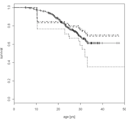
Figure 1 – The NPMLE (dashed line), the BFHE (dotted-dashed line), the INE (dotted line) based
on the partial database and the KM estimator based on the reconstructed database (solid line with marked censored times).
Figure 1 shows the NPMLE, the BFHE and the INE estimates based on the partial database and calculated using the library survival of the R software and code provided in Pan and Chappell (1998).
The NPMLE and the BFHE are very close to each other, while the INE has a clearly different shape. From Figure 1 it can be noted that the data do not exhibit the particular configuration that would set to 0 the NPMLE estimate of survival. Nonetheless, the NPMLE and the BFHE still exhibit a large drop in survival cor-responding to the earliest death. This is the underestimation problem mentioned in Section 2 and due in our case to a risk set as small as six when the first death occurs. It may be questioned whether the large drop is a real effect, and to do so we now turn to the INE. Actually, the INE also exhibits the drop, to an even higher degree. The results are puzzling: at this point, we do not know whether the NPMLE (or the BFHE) truly underestimates survival, but the INE, which is meant to correct it, estimates an even lower survival than the NPMLE.
After the results based on the partial database were obtained, the opportunity came to perform a retrospective lifetime reconstruction of all patients dead be-fore the year 2000 and mainly born after the seventies, so that it can safely be as-sumed that for them chelation therapy has been available for most of their life-time. As mentioned in Section 1, all potential patients at the end of the study are
then either dead, with death times recorded, or enrolled in the study or censored before study started. By assuming that our estimates do not change much by ex-cluding from the database those latter patients which were censored before study started (we will never be able to obtain any information about them, not even how many they were), we then obtain a database which is affected by censoring but is not affected by truncation.
Such “reconstructed” database consists of 249 patients (including the 191 of the partial database), 67 of whom (including 9 in the partial database) died before the end of study date. Table 1 shows the frequencies of censored and uncensored observations in the two databases. It should be remembered that in the partial da-tabase observations are also truncated, whereas in the reconstructed dada-tabase they are not.
TABLE 1
Summary of the two databases
Censored Dead Total
Partial database 182 9 191
Reconstructed database 182 67 249
The reconstructed database offers an important basis for comparison and lets us evaluate the relative merits of the three estimators in a real-life situation using something as close as possible to a gold standard, a rare opportunity. The quasi-gold standard, a KM estimate based on the reconstructed database, is presented in the same Figure 1 together with the NPMLE, the BFHE and the INE esti-mates, based on the partial database. There does not seem to be any trace of a sudden drop in survival at early ages: the KM estimate drops at a fairly regular pace. It may be important to recall, at this point, that KM estimates are not de-fined to the right of the latest observation, if such an observation is a censored time. That is the case in our databases, so discussion of all these estimators should not involve ages above 50 years – say – and the interpretation of the plots should be done accordingly.
The INE underestimates the gold standard at all ages (except, trivially, before the first death), whereas the NPMLE and the BFHE cross it. All three point-wise 90% confidence bands (not shown) contain the gold standard and the other two estimators for most of the significant age span, but they seem to be fairly large confidence bands, reflecting a high degree of uncertainty.
The partial database is a cross-sectional window of five years over a population with a median lifetime of more than 30 years. This is a severe case of truncation and censoring and gives rise to a very small number of observed deaths. Such a great uncertainty justifies the extra effort made by the clinical team to reconstruct the second database.
3.2. The case study: approximate sampling distributions
From a statistical viewpoint, the case study calls for a comparison of the three estimators, to investigate whether their behavior in our specific sample happens
to be unusual. To answer this question, in this section we simulate the sampling distributions of the NPMLE, the BFHE and the INE in a scenario as close as possible to the real situation of our case study. This section provides a motivation for the larger simulation study of Section 4 and can be skipped by readers not in-terested in the sampling distributions of the estimators in the case study.
Information from both the partial and the reconstructed databases is used to create the simulation setup, in particular to obtain three densities from which we simulate:
• a Weibull density fX( ;a bX, X)of the true underlying lifetimes X1, ..., XN • a Weibull density fC( ;a bC, )C of the censoring times C1, ..., CN
• a mixture density f for the truncating times TT( ) 1, ..., TN.
The density ( ; , )f y a b is said to be a Weibull with shape parameter a and scale
parameter b if 1 ( ; , ) exp ( 0), a a y y a f y a b y b b b
with survival function ( ) exp{ ( / ) }S y y b a . Simulated samples are inde- pendent. The original (before truncation) sample size is taken to be N = 249 in order to recreate an original sample similar to the reconstructed database. No-tice that, for each simulation, the final sample size n is a random variable smaller than N since, due to truncation, only observations with T Y enter the final sample.
The density fX is obtained by fitting a Weibull model under (parametric) cen-soring to the reconstructed database, using the standard survreg routine of the R software. It turns out to have shape parameter aX = 2.42 and scale parameter bX = 46.09.
The choice of the density of the censoring variable C is more difficult. We could impose that the probability P(C < X) reflects the relative proportion of censored observations in the reconstructed database, but we know that only deaths were reconstructed, not previous censored observations. The effects of such missing censored observations are underestimation of survival – even in the gold standard – and underestimation of the proportion censored P(C < X). The consequences of the former are relatively small, although difficult to quantify, but we can base the choice of the simulating density fC( ;a bC, )C on a different crite-rion. In particular, it seems important to notice that some large censoring times are present in both databases: we can keep that into account by fixing the 99-th percentile of fC( ;a bC, )C at 45 years. Similarly, the median of the censoring vari-able should be somewhat higher than the observed mean censored time in the reconstructed database: we set it to 28 years. In summary, the parameters aC, bC are chosen to be solutions of the system of equations
45 exp 0.01 28 exp 0.50 C C a C a C b b (5)
which results approximately in aC = 3.99 and bC = 30.69. As for the density of the truncating variable f , we notice that for a large proportion (176/182) of the T( ) censored observations in the partial database, the difference between C and T is equal to the duration of the study, i.e. 5 years, from 01/01/2000 to 31/12/2004. The remaining proportion of censored observations are instead lost to follow-up during the study period. Accordingly, T is taken to be equal to C − 5 with prob-ability 176/182 and equal to an independent Weibull distribution with median 23 (5 years less than the median of C) and same shape as C, otherwise. The latter is a Weibull with shape parameter 3.99 and scale parameter 25.21. The resulting mar-ginal density for T is a mixture of the density of a translated Weibull and a proper Weibull.
Censoring and truncating conditions are reconstructed in 10000 independent simulations and in each of them the NPMLE, the BFHE and the INE are com-puted. On average, the final sample size of the samples is around 200, compara-ble to the size of the partial database. Due to all choices just illustrated, we can say that with these simulations we can study approximate sampling distributions of the different estimators in conditions very similar to the partial database.
Figure 2 shows means, 5-th and 95-th percentile of their three resulting ap-proximate sampling distributions. Something unexpected can be seen: the NPMLE and the BFHE are almost exactly unbiased, whereas the INE is severely biased downward for most of the relevant range. The above-mentioned underes-timation problem slightly affects the 5th percentile of the NPMLE, but otherwise underestimation is not visible in its mean. This confirms that the two realizations of the NPMLE, the BFHE and the INE associated to the partial database are not exceptional: at least for this simulating scenario, which approximates the un-known scenario of the case study, the sampling distribution of the NPMLE and of the BFHE are better than the INE. This can be seen as a counterexample to different conclusions reached in Pan and Chappell (1998), where the INE is in-troduced mainly to correct the NPMLE. A strength of our findings is that simula-tions here approximate a real-life situation where severe truncation and censoring affect the data.
The difference in performance between the NPMLE, the BFHE and the INE seems to be due to a high percentage of censored observations, which runs around 90% in our simulations.
As Pan and Chapell (1998) themselves put, “the INE tends to slightly under-estimate thesurvival function at later times if the percentage of right-censored ob-servations is high”. We would not call the underestimation depicted in Figure 2
“slight” and we would not say it occurs only at “later” times; in any case this pos-sible explanation of the differential behavior of the two estimators deserves more investigation, as described in the next section.
Figure 2 – True underlying survival (solid) and its estimators in the simulations of Section 3.2: for
each of the three estimators NPMLE (dashed lines on the left panel), BFHE (dotteddashed line on the central panel) and INE (dotted lines on the right panel), the central line is the mean, whereas the other two lines are the 5-th and the 95-th percentiles.
4.ASIMULATION STUDY
The previous Section 3.2 contains simulations for a rather complex scenario, in which the amount of details introduced to mimic closely the conditions of our case study on thalassemia may not be of immediate interest to the general reader. We emphasize that those simulations were aimed at obtaining very realistic ap-proximations to the sampling distributions relevant for our case study and they were not general simulations performed to obtain an idea of the relative perform-ance of the different estimators. Nonetheless, we showed that in our detailed
sce-nario the INE is sub-performing with respect to the NPMLE and the BFHE, possibly due to a large (90%) percentage censored. It is interesting to investigate to what degree this behavior is reproduced in other scenarios. The large percent-age censored depends on the rather narrow time window over which the data was collected, a follow-up time of only five years. It is expected that, as the time to follow up patients increases to a wider time window, the percentage censored should decrease. To study how the percentage censored, the censoring time win-dow, the sample size and the choice of the truncating distribution affect the rela-tive performance of the nonparametric estimators, the results of several simula-tions are then presented and commented in this section.
The simulations are inspired by the case study scenario but they are a stand alone computer experiment to compare the NPMLE, the BFHE and the INE. The true lifetime distribution is taken to be Weibull with parameters 3 and 50 in all cases, similar to the one fitted to our data, just with parameters rounded up. This way, our simulations keep a realistic flavor since they can then be thought of as simulated human lifetimes for patients affected by a life-threatening disease.
Regarding the truncating and censoring mechanisms, we imagine a calendar time origin when study begins (just like the day 01/01/2000 in our case study), we then simulate a date of birth (DOB) by simulating the truncating variable T going backward in time, so that
DOB = time origin - T;
finally we consider several different time windows to follow up the patients, start-ing from five years as in our thalassemia case study and up to 35 years. To sim-plify things, we assume no new births and no patients lost to follow-up during the study period.
We consider a Weibull truncating distribution for T with parameters 4 and 25 in Subsection 4.1 and a Uniform truncating distribution between 0 and 40 in Sub-section 4.2, to check whether the effects seen for the Weibull are robust to the choice of the truncating distribution.
For both choices of the truncating distribution, we first vary the time window from five years up as explained above; we then consider what happens for larger sample sizes when the time window is kept fixed at 5 years. Of course, these are only few among the infinite scenarios one can imagine, but we focus on these since they represent realistic viable variations of the design we used in our case study. Qualitatively similar results can be obtained by varying the parameters of the truncating Weibull distribution within a realistic range, but the simulations are not shown for the sake of conciseness.
For each scenario, 10000 simulation runs are generated and two measures of performance of the different estimators are computed: the integrated absolute er-ror (IAE) and the integrated average width (IAW).
IAE is defined as 50
0| ( )S t W t dt( )|
where S is, in turn, the average (over the simulation runs) of the NPMLE, of the BFHE and of the INE and W is the survival function corresponding to the true Weibull density fX. IAE is a measure of bias when using estimator S to estimate W. Notice that the integral is computed up to the age t = 50 in order to avoid
problems with undefined NPMLE in the upper tail; when the last observation is censored and smaller than 50, the last defined estimate is carried forward to
t = 50. IAW is defined as 50 95 05 95 05 0 max{ ( ), ( ), ( )} min{ ( ), ( ), ( )} IAW
S t W t S t S t W t S t dtwhere S95 and S05 are the 95-th and 5-th pointwise percentiles of the simulated NPMLE, BFHE and INE. Notice the use of max and min to account for possi-ble crossing phenomena such as the one depicted in Figure 2; for example, when the central 95% of the sampling distribution does not cover true survival, as the INE does around 50 in that picture, the contribution to IAW should be large. Al-though other choices are certainly possible, IAW is a measure of variability of the sampling distribution of the estimator S.
4.1. Simulations with truncating Weibull distribution
The densities we simulate X and T from in this section are:
– a Weibull density f X( ;3,50) for the true underlying lifetimes X1, ..., XN – a Weibull density f T( ;4, 25) for the truncating times T1, ..., TN.
If Ti Xi the simulated patient enters the study at age Ti (i.e. is not truncated) and is followed up for a time window lasting w years. If, in addition,
i i i
T X T , then the patient is dead and a death time is produced, other-w
wise a censored observation.
Table 2 contains simulated IAE and IAW when the follow-up time window is varied between w = 5 and w = 35. The original sample size is fixed to 250 and it reduces to 224 on average, due to truncation. The resulting average percentage censored resulting from these combinations decreases from 93% to 26% as the follow-up time window increases.
The first important result to notice is that the bias of the NPMLE, measured by IAE, is smaller than the bias of the INE in all scenarios. As for the average width of the confidence intervals, the INE starts showing a better performance that the NPMLE only when the percentage censored becomes smaller than 50%, which happens when the follow-up window is around 20 years or more. Notice that 20 years is a fairly long time even for well-funded studies.
As for the comparison between NPMLE and BFHE, they are fairly equivalent: it appears that the NPMLE dominates the BFHE with regard to bias (IAE), whereas the opposite happens when we consider the width of the estimating in-tervals (IAW).
TABLE 2
Simulation results on bias (IAE) and variability (IAW) of several estimators under Weibull truncation and follow-up lasting w years
IAE IAW w(yrs) Original s.s Ave. final s.s Ave. % Cens.
NPMLE BFHE INE NPMLE BFHE INE
5 250 224 93 0.74 1.09 5.27 12.05 10.16 12.28 6 250 224 91 0.47 0.81 4.68 11.54 9.85 11.68 7 250 224 89 0.4 0.69 4.19 10.62 9.26 11.09 8 250 224 87 0.31 0.57 3.77 9.75 8.61 10.43 9 250 224 85 0.23 0.47 3.38 9.1 8.14 9.91 10 250 224 83 0.18 0.39 3.02 8.43 7.69 9.38 11 250 224 81 0.11 0.3 2.7 7.97 7.39 8.97 12 250 224 79 0.12 0.28 2.36 7.48 7.05 8.59 13 250 224 77 0.05 0.2 2.12 7.13 6.85 8.28 14 250 224 74 0.05 0.19 1.84 6.84 6.61 8 15 250 224 72 0.05 0.17 1.58 6.55 6.35 7.62 20 250 224 60 0.05 0.14 0.6 5.89 5.75 6.35 25 250 224 48 0.05 0.13 0.21 5.7 5.56 5.6 30 250 224 36 0.05 0.13 0.09 5.73 5.58 5.24 35 250 224 26 0.09 0.17 0.22 5.58 5.44 4.95
When the original sample size varies instead from 250 to 2000 and the follow-up window is kept constant at w = 5 years, we obtain the results in Table 3. The final sample size after truncation increases accordingly, whereas the percentage censored is stable around 93%.
The results confirm the ones obtained for the case study: due to the high per-centage censored, the INE behaves worse than the NPMLE and the BFHE for all sample sizes considered, in terms of both bias (IAE) and variability (IAW). The NPMLE seems to have smaller bias but larger variability than the BFHE.
In addition, notice that the bias of the INE seems to stabilize above 5 no mat-ter what the sample size is, whereas for both the NPMLE and the BFHE the bias decreases as the sample size increases. In other words, for the INE we suspect lack of consistency.
TABLE 3
Simulation results on bias (IAE) and variability (IAW) of several estimators under Weibull truncation and varying original sample size
IAE IAW w(yrs) Original s.s Ave. final s.s Ave. % Cens.
NPMLE BFHE INE NPMLE BFHE INE
5 250 224 93 0.68 1.04 5.28 12.28 10.37 12.34 5 260 233 93 0.66 1.01 5.33 12.15 10.29 12.31 5 270 242 93 0.64 0.98 5.37 12.01 10.17 12.32 5 280 250 93 0.62 0.96 5.42 11.9 10.06 12.31 5 290 259 93 0.57 0.92 5.45 11.74 9.91 12.23 5 300 268 93 0.65 0.98 5.46 11.6 9.8 12.2 5 350 313 93 0.55 0.86 5.56 11.1 9.42 12 5 400 358 93 0.5 0.79 5.68 10.66 9.06 11.87 5 450 403 93 0.53 0.8 5.67 10.19 8.68 11.69 5 500 447 93 0.47 0.74 5.7 9.91 8.42 11.51 5 600 537 93 0.43 0.67 5.75 9.34 7.99 11.22 5 700 626 93 0.42 0.64 5.8 8.82 7.59 11.04 5 800 716 93 0.36 0.58 5.83 8.55 7.3 10.9 5 900 805 93 0.36 0.55 5.82 8.17 7 10.67 5 1000 895 93 0.3 0.49 5.82 8.08 6.92 10.56 5 2000 1789 93 0.22 0.36 5.82 6.33 5.47 9.45
4.2. Simulations with truncating uniform distribution
To check whether the conclusions reached using a Weibull density for the truncating variable are sensitive to the choice of such density, we consider briefly in this section a truncating random variable T uniformly distributed between 0 and 40 years.
The simulation scenarios are less dense than before for the sake of concise-ness: when the follow-up time window is varied we obtain the results shown in Table 4, when the original sample size varies we obtain Table 5. In both cases we can say that the conclusions are similar to the ones obtained for the Weibull trun-cating density in the previous section, with the BFHE being overall better than both the NPMLE and the INE in terms of width in all scenarios, and loosing to the NPMLE in terms of bias. In none of the cases considered does the INE per-form better.
TABLE 4
Simulation results on bias (IAE) and variability (IAW) of several estimators under Uniform truncation and varying follow-up years
IAE IAW w(yrs) Original s.s Ave. final s.s Ave. % Cens.
NPMLE BFHE INE NPMLE BFHE INE
5 250 222 94 0.34 0.53 5.54 9.35 9.08 12.11
10 250 222 86 0.03 0.12 2.75 6.51 6.42 7.84
20 250 222 66 0.01 0.05 0.51 4.74 4.71 5
30 250 222 44 0.01 0.03 0.11 4.31 4.29 4.37
TABLE 5
Simulation results on bias (IAE) and variability (IAW) of several estimators under Uniform truncation and varying original sample size
IAE IAW w(yrs) Original s.s Ave. final s.s Ave. % Cens.
NPMLE BFHE INE NPMLE BFHE INE
5 300 267 94 0.33 0.47 5.71 8.48 8.26 11.64 5 400 355 94 0.32 0.42 5.84 7.45 7.28 10.94 5 500 444 94 0.32 0.42 5.83 6.6 6.49 10.38 5 1000 889 94 0.32 0.38 5.52 4.74 4.69 8.74 5 2000 1777 94 0.3 0.33 5.03 3.42 3.4 7.31 5. CONCLUSIONS
We have started from a case study of applied interest per se, the estimation of overall survival of thalassemia major patients. We then have taken advantage of the existence of a partial database and of a more complete reconstructed database to simulate the entire sampling distributions of the NPMLE, the BFHE and the INE for our case study, which is characterized by severe truncation and censoring.
The case study has suggested more general simulations that allow us to discuss the relative merits of the NPMLE, the BFHE and the INE. We suggest not to use the INE when the percentage censored is higher than 50% and we present some evidence regarding the possible lack of consistency of the INE as the sam-ple size increases. As for the NPMLE and the BFHE, there are no major differ-ences, the NPMLE being less biased, but more unstable, than the BFHE.
ACKNOWLEDGMENTS
The authors thank the personnel of the Centro Microcitemie of the University of Tu-rin for allowing the use of their data. The authors also thank Novartis Italy for financial support and MIUR (the Italian Ministry of Education, Universities and Research) PRIN 2007 “Statistical methods for learning in clinical research”, for partial funding. An anonymous referee provided useful comments.
Department of Mathematics MAURO GASPARINI
Politecnico di Torino – Italy
Centro regionale per l’epidemiologia e la salute ambientale MARTINA GANDINI
ARPA Piemonte – Grugliasco, Italy
REFERENCES
C.BORGNA-PIGNATTI (2006).Thalassemia.A few new tiles in a large mosaic. “Haematologica/the hematology journal”,91(9): 1159-1162.
H.FRYDMAN (1994).A note on nonparametric estimation of the distribution function from
interval-censored and truncated observation.“Journal of the Royal Statistical Society”, Series B, 56:
71-74.
M. GASPARINI(1996).Nonparametric Bayes estimation of a distribution function with truncated data. “Journal of statistical planning and inference”, 55: 361-369.
E.L. KAPLAN, P. MEIER(1958).Nonparametric Estimation from Incomplete Observations.“Journal of the American Statistical Association”, 53: 457-481.
N. KEIDING, R.D. GILL(1990).Random truncation models and markov processes.“The Annals of Statistics”, 18(2): 582-602.
W. PAN, R. CHAPPELL(1998).A Nonparametric Estimator of Survival Functions for Arbitrarily
Trun-cated and Censored Data.“Lifetime Data Analysis” 4: 187-202.
R DEVELOPMENT CORE TEAM (2005).R: A language and environment for statistical computing.R Foundation for Statistical Computing, Vienna, Austria. ISBN 3-900051-07-0, URL: http://www.R-project.org.
W-Y. TSAI, N.P. JEWELL, M-C. WANG(1987).A note on the product-limit estimator under right censoring
and left truncation.“Biometrika”, 74: 883-886.
BW. TURNBULL(1976).The empirical distribution function with arbitrarily grouped, censored and
trun-cated data.“Journal of the Royal Statistical Society”, Series B, 38(3): 290-295.
S. WELLEK(1990). A nonparametric model for product-limit estimation under right censoring nd left
truncation.“Communications in Statistics: Stochastic Models”, 6(4): 561-592.
SUMMARY
A comparison of nonparametric estimators of survival under left-truncation and right-censoring motivated by a case study
We present an application of nonparametric estimation of survival in the presence of left-truncated and right-censored data. We confirm the well-known unstable behavior of the survival estimates when the risk set is small and there are too few early deaths.
How-ever, in our real scenario where only few death times are necessarily available, the proper nonparametric maximum likelihood estimator, and its usual modification, behave less badly than alternative methods proposed in the literature. The relative merits of the dif-ferent estimators are discussed in a simulation study extending the settings of the case study to more general scenarios.