1
A Spatial Panel Wage Curve for Spain
1Raul Ramos ([email protected])
AQR-IREA, Universitat de Barcelona
Catia Nicodemo ([email protected])
CHESO & Department of Economics, University of Oxford
Esteve Sanromá ([email protected])
IEB & Universitat de Barcelona
Abstract
Most empirical studies on the Spanish wage curve have ignored the possible spatial interaction
effects between the regions. This paper reconsiders the Spanish wage curve using more recent data
than previous studies and taking into account the role of regional spillovers. From a methodological
perspective, we apply the two-step procedure proposed by Bell et al (2000) to estimate a dynamic
wage curve with spatial spillovers. In a first stage, we use microdata from the Spanish Social
Security Records (Muestra Continua de Vidas Laborales) to obtain composition-corrected wages
that are used in a second stage to estimate a wage curve over the period 2000-2010 allowing for
spatial effects of unemployment across regions. Opposite to previous studies, we find that the wage
equation is highly autoregressive and that regional spillovers are relevant to explain the relationship
between unemployment and wages in the Spanish provinces.
Keywords: Spatial panel, wage curve, unemployment, Spanish regional labour markets.
JEL Codes: J31, J64, R23
1 The research leading to these results has received funding from the European Community's Seventh Framework Programme (FP7/2010-2.2-1) under grant agreement nº 266834.
2
1. Introduction and objectives
During the first half of the nineties, Blanchflower and Oswald (1990, 1994a, 1994b, 1995) developed an ambitious research program on the relationship between individual wages and local unemployment rates using several databases for a wide set of countries at the individual level. The main result of these studies was the finding of an empirical regularity, which was called “the wage curve”. This curve establishes an inverse relationship between individual wages and the local unemployment rate. More precisely, a worker living in an area of high unemployment earns a lower wage than those with identical characteristics living in an area with less unemployment. A more surprising result is that the elasticity of wages to unemployment is very close to –0.10, a value that is quite stable among countries –with diverse institutional frameworks-, among a range of time periods and for distinct samples or databases. Blanchflower and Oswald (2005) updated the analysis for the US labour market and found similar results. This finding contradicts macroeconomic studies which have concluded that one of the causes of European unemployment during the eighties and nineties was its relatively low wage flexibility when compared to the United States, Japan or Canada (Layard, Nickell and Jackman, 1991). In fact, this result seems to be quite robust as shown by Nijkamp and Poot (2005). These authors applied meta-analytic techniques on a sample of 208 elasticities for 30 countries derived from 17 different studies published between 1990 and 2001 and they found that an unbiased mean estimate (i.e., accounting for study heterogeneity such as the use of grouped versus microdata or disaggregated gender analysis) of the wage curve elasticity is about –0.07. Babecky et al. (2008) extended the research by Nijkamp and Poot (2005) by compiling a larger number of studies (64) and estimates (more than 1400) but, more interestingly, to consider a larger number of countries (41) and more recent time periods including studies published since 2001 up to 2007. The analysis of more recent works was particularly relevant as wage curve estimates were available for a wider set of emerging economies and economies in transition (having clearly different institutional frameworks), but also to consider the potential effect of labour market reforms carried out in the 1990s. They conclude that there is evidence of significant differences among countries, time periods and groups of workers that cast doubt on the generalised validity of the “wage curve empirical law”.
In the most recent years, the research on this topic has advanced along two parallel lines: consolidating the theoretical basis of the wage curve and considering different approaches to the specification of the wage curve.
From a theoretical perspective, the negative relationship between wages and regional unemployment is contradictory –at least, at first sight- with the theory of compensatory wage differences as given initially by Adam Smith and more formally expressed at the territory level by Harris and Todaro (1970) and by Hall (1972). According to the latter, there is a positive relationship between the two variables: the wage rate is higher in the areas of high unemployment to equalize annual earnings or wages plus unemployment insurance, in the different regions. So, the theoretical foundations of the wage curve are related to non-competitive labour market models. In particular, earlier works have offered a wide variety of explanatory
3
models, including implicit contracts, union bargaining, efficiency wages, and labour turnover costs (Blanchflower and Oswald, 1994b; Campbell and Orszag, 1998; Montuenga and Ramos, 2005; Campbell, 2008). However, there is currently a wide consensus that the most plausible explanations are related to efficiency wages and/or labour turnover costs (Blien et al., 2013).
From a methodological perspective, recent studies are increasingly using dynamic panel data using different methods to control for composition effects and spatial econometric techniques to account for inter-regional spillovers. As Longhi et al. (2006) highlight much of the existing wage curve literature have considered local labour markets as nonspatial “replications” of labour market outcomes within the national economy. However, if the wage curve is related to worker heterogeneity and monopsonistic competition, employment opportunities in surrounding regions and the interregional cost of commuting or migration also matter to explain the relationship between unemployment and wages. Longhi et al. (2006) found that spatial effects matter in the wage curve for Western Germany, an aspect that was found by the early work of Buettner (1999) and that has been reconfirmed by Elhorst et al. (2007) for East Germany and by Falk and Leoni (2011) for Austria.
From this perspective, the analysis of the wage-local unemployment relationship for Spain is especially relevant because of the institutional characteristics of its labour market. Although recent reforms have tried to improve the functioning of the Spanish labour market, during the last decades it has been characterised by an intermediate collective bargaining system with high coverage, high firing costs, a quite generous benefit system, and a very high volatility of employment with very high rates of unemployment during economic crisis. Consequently, a low elasticity of wages to unemployment or even the absence of a wage curve is expected. However, fixed-term contracts represent a very important share of the total private sector employees, implying a high turnover, and a certain monopsonistic power of firms to settle wages according to the evolution of the unemployment rate. An additional reason to analyse the relationship between wages and local unemployment for Spain is the limitations of previous studies on this topic in the light of this recent literature.
The results from earlier studies of the Spanish wage curve did not deviate significantly from the international previous literature (see, for instance, Canziani, 1997; García-Mainar and Montuenga-Gómez, 2003; Montuenga et al., 2003; or Sanromá and Ramos, 2005). Recent studies have, however, started to consider the use of more sophisticated econometric methods and spatial aspects of the wage curve. In particular, Garcia-Mainar and Montuenga (2012) have estimated a dynamic wage curve for Spain, using panel data coming from the eight waves of the European Community Household Panel (ECHP) for the period 1994 to 2001. Estimated results seem to reveal that, contrary to most earlier empirical research for other countries, a static wage curve models fits well the case of Spain, since the autoregressive parameter is non-significantly different from 0, and with the elasticity wages to unemployment of -0.07. This can be interpreted as wages being low-degree sensitive to changes in unemployment, but wages adjusting very rapidly to such changes, at least during the period under consideration. However, as authors recognise this result must be treated with caution, given that the period analysed, first, may be too short to capture the
4
dynamic behaviour of wages and, second, coincides with an expansive phase of the Spanish economy, during which unemployment fell sharply, employment increased strongly, and real wage growth was controlled. Bande et al. (2012) have estimated regional wage equations for the Spanish regions using data from the Structure of Earnings Survey for 1995, 2002 and 2006 and considering the spatial heterogeneity of the curve. Although they work with only 3 groups of regions, their results show clear differences with regions with higher unemployment rates exhibiting a lower wage flexibility. This evidence is consistent with the model of collective bargaining in Spain because it reflects the important imitation effects that generate a weak sensitivity of individual wages to local labour market conditions.
Taking this previous research as a starting point, the objective of the paper is twofold: first, to test the validity of the wage curve when considering more recent data for Spanish regions including a long expansion period from 2000 to 2007 and the first years of the economic crisis up to 2010 that have been characterised by a fast and strong increase in unemployment rates and, second, to analyse the robustness of the results to a wage curve specification based on a dynamic panel with spatial spillovers. In particular, our study focuses on Spanish NUTS III provinces using microdata from the Muestra Continua de Vidas Laborales (MCVL) and recently developed spatial econometric panel data techniques will be applied to estimate a dynamic wage curve including interregional spillovers. The main advantage of using panel data in relation to the use of cross-sectional data is that it permits to control for unobservable heterogeneity by the inclusion of individual, regional and time fixed effects. Moreover, although space has always played an important role in this literature, the existence of regional linkages have not been taken into account until some recent studies (Longhi et al., 2006; Elhorst et al., 2007) and no previous evidence exists for Spain. If spatial dependence is present (as it is expected to be on regional data), it should be removed from data because the violation of independence assumption may lead to misleading conclusions. The use of spatial econometrics techniques will permit to overcome this problem.
The rest of the paper is structured as follows: first, we described the data sources used in the analysis; second, the applied methodology is described and, next, we focus on the obtained empirical evidence. Last, the paper ends with some final remarks and ideas for further research.
2. Data
To design our study, we use the seven waves of the Continuous Sample of Working Histories (Muestra Continua de Vidas Laborales; hereafter MCVL) from 2004 until 2010. The data come from the registry of the Social Security System (SSS) for active people in the labour market and provides information on the computerized records of the Spanish Social Security and the Continuous Municipal Register. Since 2004, this database has provided annual information on more than one million people who have had some kind of work relationship with the Social Security every year, regardless of the duration or the nature of the relationship. It is an administrative data set with longitudinal information for a 4% non-stratified random
5
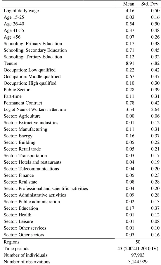
sample of the population who are affiliated with Spain's SSS). The MCVL is only representative of the population related to the SSS in the year of extraction, and it is not representative of the past: although it contains information on previous social security contributions by the individuals selected. So far, the MCVL reproduces the labour history of the affiliated starting from their first job. The MCVL is an appropriate database to study the labour market in Spain and, in fact, has several advantages when compared with other data sources such as for example the Wage Structure Survey (WSS), because it provides more a higher territorial detail (the MCVL reports residential data at the level of municipality) and it has a longitudinal structure (for more details about the MCVL, see García-Perez, 2008). The data set provides information of all of the historical relationships of any individual with the SSS (in terms of work and unemployment benefits). We have also information regarding the type of contract, sector of activity, qualification and earnings, date when entering or leaving the job market, part-time or full-time status and firm size. Moreover, the database contains information on gender, nationality, country of birth, residence, date of birth and level of education. In addition, the MCVL gives details about the establishment (location, number of workers, industry and sector) in which a worker is hired. The temporal dimension of the MCVL panel (2005-2010) allows us to track the entry in the labour market of individuals and permits to avoid the attrition problem that we obtain when we to study the entries and exits of individuals in the job market using only one wave and looking back in the past of the worker relationship with the SSS. To build our sample we have merged the wave of 2010 with the wave from 2009 until 2005, and since we know all the work history of workers we go back until 2000. Considering years before to 2000 increase the risk of attrition, because the database is not representative at these years but only for the years where extraction is done. We have deleted people that not report a labour relation with the SSS. The main outcome variable of interest in our dataset is the wage of Spanish people. The MCVL has information on monthly earning paid mandatory to pension schemes of SSS and the days worked. Based on this information we calculate the logarithm of the daily wage. Regarding wages, we have used the daily wage, calculated as the ratio of annual earnings to days worked. We have eliminated observations when the daily earnings were below the minimum base or exceeded the maximum base to avoid the problem of censured data. As unemployment data by provinces from the Instituto Nacional de Estadística (INE)’s Labour Force Survey that are required in our second step estimation are only available at the quarterly frequency, only four data points per year could be used. In particular, we have kept people who report a wage in February, May, August or November for more than 2 years in the considered period. This allows us to take in consideration the seasonality across the year. In addition, this permits to include individual fixed effects in the first stage of our modelling approach. If the individual reported more than one job, we take the one with greatest earning. Quarterly averages of provincial Consumer Price Indexes used to deflate wages were obtained from INE. We have only considered individuals from 15 to 65 years old and we have taken a random sample of 97903 individuals with a total of 3.144.929 observations. Table 1 depicts the summary description of the variables that will be used to estimate the wage equation. In particular, apart of daily wages, we consider age, schooling levels, tenure, occupation, public sector worker, part-time, permanent contract, firm size (proxied by the number of workers in the firm), activity sector and province of residence (NUTS III regions).
6
Table 1. Descriptive statistics
Mean Std. Dev.
Log of daily wage 4.16 0.50
Age 15-25 0.03 0.16
Age 26-40 0.54 0.50
Age 41-55 0.37 0.48
Age +56 0.07 0.26
Schooling: Primary Education 0.17 0.38
Schooling: Secondary Education 0.71 0.45
Schooling: Tertiary Education 0.12 0.32
Tenure 8.91 6.82
Occupation: Low qualified 0.22 0.42
Occupation: Middle qualified 0.67 0.47
Occupation: High qualified 0.10 0.30
Public Sector 0.28 0.39
Part-time 0.11 0.31
Permanent Contract 0.78 0.42
Log of Num of Workers in the firm 3.54 2.64
Sector: Agriculture 0.00 0.06
Sector: Extractive industries 0.01 0.12
Sector: Manufacturing 0.11 0.31
Sector: Energy 0.16 0.37
Sector: Building 0.05 0.22
Sector: Retail trade 0.05 0.21
Sector: Transportation 0.03 0.17
Sector: Hotels and restaurants 0.04 0.19
Sector: Telecommunications 0.04 0.20
Sector: Finance 0.05 0.23
Sector: Real state 0.08 0.28
Sector: Professional and scientific activities 0.04 0.20 Sector: Administrative activities 0.09 0.28
Sector: Public administration 0.02 0.13
Sector: Education 0.17 0.37
Sector: Health 0.01 0.12
Sector: Leisure 0.01 0.08
Sector: Other services 0.01 0.10
Sector: Other sectors 0.03 0.16
Regions 50
Time periods 43 (2002.II-2010.IV)
Number of individuals 97,903
7
3. Methodology
The specification of the wage curve used by Blanchflower and Oswald (1990, 1994a, 1994b, 1995) consisted in regressing the logarithm of individual wages on a number of control variables related to personal and job characteristics and the regional unemployment rate. However, a difficulty arises because this equation includes an explanatory variable of interest (the regional unemployment rate) that is defined at a higher level of aggregation than the dependent variable (individual). As Moulton (1986) shows, the estimation of this kind of equation will bias upward the values of the test of individual significance for this variable. Moreover, the inclusion of additional variables in order to correct for the possible omission of relevant variables at the regional level usually induces collinearity problems. For these reasons, more recent studies usually follow a two-step procedure as in Bell et al. (2002). The first step consists of a Mincer equation estimated at the individual level, including time-varying, individual fixed effects and regional dummies. These dummies can be interpreted as average wages in the local labour market, corrected for composition effects. In particular, the logarithm of wages was regressed on a number of control variables related to personal and job characteristics together with the regional dummies:
𝑙𝑛(𝑤𝑖𝑟𝑡) = 𝛼𝑍𝑖𝑟𝑡+ 𝛾𝑡+ 𝛿𝑟𝑡+ 𝜏𝑖+ 𝜀𝑖𝑟𝑡 (1) where 𝑙𝑛(𝑤𝑖𝑟𝑡) is the natural logarithm of the wage of the individual i that lives in region r at time t, 𝑍𝑖𝑟𝑡 is a set of individual factors that can affect wages of the individual, such as the level of schooling, his/her experience or other characteristics such as occupation, 𝛾𝑡 is a time trend that control for all common shocks to the considered regions while 𝛿𝑟𝑡 are region specific effects that can be interpreted as average wages in region r at time t corrected for composition effects. As each individual is observed at least for 2 periods, individual fixed effects (𝜏𝑖) have also been included in equation to control for time-invariant unobserved heterogeneity. This implies, however, that some usual controls in the Mincer equation such as gender cannot be included when estimating equation (1). Finally, 𝜀𝑖𝑟𝑡 is a random error term which follows a normal distribution with zero average and constant variance.
In the second step, the wage curve is estimated using the composition corrected wages, 𝛿𝑟𝑡 obtained in the first step, as the endogenous variable and the natural logarithm of the regional unemployment is introduced as explanatory variable together with time and regional fixed effects:
𝛿̂ = 𝛽 ln(𝑢𝑟𝑡 𝑟𝑡) + 𝛾𝑡+ 𝛿𝑟+ 𝑣𝑟𝑡 (2) As highlighted by Longhi et al. (2006) and Elhorst et al. (2007), most empirical analysis of the wage curves assume that regions are isolated economies. However, theoretical and empirical arguments suggest that regions, as well as not being homogeneous, are also not independent. From a theoretical point of view, the labour market conditions in neighbouring regions could influence commuting and/or migration decisions that, at the same time, could affect wage bargaining in the considered region (see, for instance, Longhi, 2012). Moreover, from an empirical perspective and as highlighted by Elhorst (2003), if the influence of spatial linkages is ignored, results could be biased and hence conclusions could be misleading. For this reason, equation (2) is augmented including the possibility that the evolution of unemployment in
8
neighbouring regions could also affect wages in the considered regions. Recent studies adopting a similar approach incorporate substantive spatial dependence, meaning that spatial effects propagate to neighbouring regions by means of endogenous as well as exogenous variables. Taking this into account, equation (3) is augmented including the spatial lag of the endogenous variable (values of the endogenous variable observed in neighbouring regions), but also of the regional unemployment rate:
𝛿̂ = 𝜇 ∑𝑟𝑡 𝑁𝑗=1𝑚𝑗𝑟𝛿̂𝑟𝑡+ 𝛽 ln(𝑢𝑟𝑡) + 𝜃 ∑𝑁𝑗=1𝑚𝑗𝑟ln(𝑢𝑟𝑡)+ 𝛾𝑡+ 𝛿𝑟+ 𝑣𝑟𝑡 (3) Where 𝜇 is the spatial autoregressive coefficient, 𝜃 is the parameter associated to regional spillovers in the unemployment rate and 𝑚𝑗𝑟 is each of the elements of the spatial weights matrix M2 that describes the spatial arrangement of the different regions. In our empirical analysis, we will consider two different time-invariant spatial weight matrixes: first, a binary contiguity matrix has been used, and second, geographical distance has been used to define the elements of M, more precisely the inverse of great-circle distance3 between
province capitals4, which is exogenous to the analysed relationship5. As usual in the literature, and in order to
normalize the outside influence upon each region, in both cases, the weight matrix has been standardized such that the elements of a row sum up to one.
Last, and following Baltagi et al (2009 and 2012), equation (3) is enlarged with the lag of the composition corrected wages to account for wage inertia:
𝛿̂ = 𝜆𝛿𝑟𝑡 ̂ + 𝜇 ∑𝑟𝑡−1 𝑁𝑗=1𝑚𝑗𝑟𝛿̂𝑟𝑡+ 𝛽 ln(𝑢𝑟𝑡) + 𝜃 ∑𝑗=1𝑁 𝑚𝑗𝑟ln(𝑢𝑟𝑡)+ 𝛾𝑡 + 𝛿𝑟+ 𝑣𝑟𝑡 (4) The next section shows the results of estimating models described up to now.
4. Results
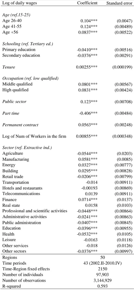
In this section, we present the results of estimating the models discussed in the previous one. In particular, the results of estimating equation (1) by panel data fixed effects are shown in Table 2. As we can see in Table 2, variables related to educational levels and tenure were significant and showed the expected signs, detecting a positive relationship between human capital and wages. Concerning the individual of reference, workers with educational levels above elementary levels receive higher wages. The accumulation of professional experience also has a positive effect on wages. People who work only part-time received significantly lower wages than those who work full-time. The dummy variables related to the occupations expressed the effect of job characteristics as well as the additional required qualification. We had taken low qualified jobs as the base category. The estimation results showed that, when controlling for other factors, workers in high qualified jobs earned about significantly more. The information related to industry sectors
2 Although the spatial weight matrix is usually denoted by W, here and in order to avoid confusion with wages, we follow the notation by Kelejian and Robinson (1997) and the spatial weight matrix is denoted by M.
3 The great-circle distance is the shortest distance between any two points on the surface of a sphere and it has been computed using
STATA’s globdist command.
4 Latitude and longitude data for capital cities of the Spanish provinces have been obtained from the Instituto Geográfico Nacional
(http://www.ign.es/ign/es/IGN/BBDD_GRAVIMETRICO.jsp).
5 The results are robust to different specifications of the matrix such as the inverse of the distance to the square. The detailed results
9
permitted, on the one hand, to control for the effect of the various productive and employment structures in the various provinces and, on the other, to provide more information about job characteristics not previously considered.
In equation (2), we use the estimates of time-varying region specific effects from equation (1) as the endogenous variable and the natural logarithm of the regional unemployment is introduced as explanatory variable together with time and regional fixed effects.
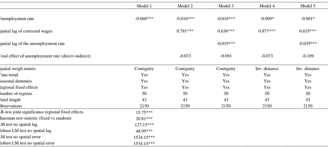
The results of estimating equation (2) are shown in Table 3. In this sense, it is worth mentioning that, although our empirical specifications incorporate regional externalities on the basis of theoretical considerations, we apply the usual modelling approach: first, we have started estimating a basic specification, without spatial lags of the endogenous or the exogenous variables and including time-period and regional fixed effects. Second, a Hausman test to select between fixed and random effects and the joint significance of the effects has been calculated. Next, we have computed the LM and robust LM statistics (proposed by Anselin et al (2006) and adapted by Elhorst (2009) to the context of panel data) in order to test for the null hypothesis of no spatial lag of the endogenous variable and no spatial error in the models. In the case that both groups of tests lead to the non-rejection of the null hypothesis, this will imply that there are no geographical spillovers in the wage curve. However, in case the null hypothesis of no spatial lag or no spatial error is rejected, then it will be necessary to include a spatial lag of corrected wages or to consider a spatial error model, respectively.
Column 1 of table 3 shows the results of estimating the basic specification of the wage curve including regional fixed effects, a time trend and seasonal dummies (equation 2). The model is estimated by GMM following the Arellano and Bond (1998) proposal for dynamic panel models. According to these estimates, we find an elasticity of wages to unemployment of -0.068, lower than the value found by Blanchflower and Oswald (1994) but close to the value found in the meta-analysis by Nijkamp and Poot (2005). A Hausman test for choosing between the random and the fixed effect specification clearly discriminates in favour of the latter and the LR test clearly rejects the hypothesis of the no joint significance of the regional fixed effects. If we look at the results of the LM and robust LM tests using the spatial weight matrix based on contiguity, the LM test for no spatial error rejects the null at the 1% significance level while the robust test for no spatial lag rejects it any significance level, while the robust test is also more significant for no spatial lag. Taken into account the results of these tests, as there are problems of spatial dependence, the estimates are inconsistent (Anselin, 1988).6
6 We have applied STATA procedures for the estimation of spatial panel data models and dynamic spatial panel data models
implemented by Belotti, Hughes and Mortari (xsmle version 1.4 17 Mar 2013) and by Shehata and Mickaiel (2012 and 2013). (spglsxt 9 Dec 2012 and spregdhp, 21 Mar 2013).
http://ideas.repec.org/c/boc/bocode/s457610.html http://ideas.repec.org/c/boc/bocode/s457421.html http://ideas.repec.org/c/boc/bocode/s457505.html
10
Table 2. Mincer equation - Robust Panel Data Fixed Effects estimates
Log of daily wages Coefficient Standard error
Age (ref.15-25)
Age 26-40 0.104*** (0.0047)
Age 41-55 0.124*** (0.00489)
Age +56 0.0837*** (0.00522)
Schooling (ref. Tertiary ed.)
Primary education -0.0410*** (0.00516)
Secondary education -0.0376*** (0.00291)
Tenure 0.00255*** (0.000199)
Occupation (ref. low qualified)
Middle qualified 0.0801*** (0.00567)
High qualified 0.0831*** (0.00424)
Public sector 0.123*** (0.00708)
Part time -0.406*** (0.00484)
Permanent contract 0.0563*** (0.00248)
Log of Num of Workers in the firm 0.00855*** (0.000348)
Sector (ref. Extractive ind.)
Agriculture -0.0544*** (0.0203) Manufacturing 0.0581*** (0.0085) Energy 0.0327*** (0.00777) Building 0.0295*** (0.00828) Retail trade -0.0206*** (0.00799) Transportation -0.014 (0.00911)
Hotels and restaurants -0.00193 (0.00869)
Telecommunications 0.0139 (0.00911)
Finance 0.0714*** (0.0137)
Real state 0.0158 (0.0103)
Professional and scientific activities -0.0448*** (0.00864) Administrative activities -0.0241*** (0.00863) Public administration -0.0407*** (0.00845) Education -0.0396*** (0.00955) Health -0.0532*** (0.0105) Leisure -0.0163 (0.0118) Other services -0.018 (0.0126) Other sectors -0.0376*** (0.00997) Regions 50
Time periods 43 (2002.II-2010.IV)
Time-Region fixed effects 2150
Number of individuals 97,903
Number of observations 3,144,929
11
Table 3. Static wage curve with regional spillovers
Model 1 Model 2 Model 3 Model 4 Model 5
Unemployment rate -0.068*** -0.016*** -0.016*** -0.009* -0.001*
Spatial lag of corrected wages 0.781*** 0.636*** 0.877*** 0.635***
Spatial lag of the unemployment rate -0.019*** -0.039***
Total effect of unemployment rate (direct+indirect) -0.073 -0.091 -0.073 -0.109
Spatial weigh matrix Contiguity Contiguity Contiguity Inv. distance Inv. distance
Time trend Yes Yes Yes Yes Yes
Seasonal dummies Yes Yes Yes Yes Yes
Regional fixed effects Yes Yes Yes Yes Yes
Number of regions 50 50 50 50 50
Panel length 43 43 43 43 43
Observations 2150 2150 2150 2150 2150
LR-test joint significance regional fixed effects 15.75***
Hausman test-statistic (fixed vs random) 20.81***
LM test no spatial lag 127.15***
Robust LM test no spatial lag 48.99***
LM test no spatial error 1534.15***
Robust LM test no spatial error 1534.14***
12
Column 2 of table 3 shows the results obtained when including the spatial lag of the endogenous variable using the spatial weight matrix based on contiguity (equation 3) and applying the GMM method proposed by Han and Phillips (2010) for spatial dynamic panels. The results are not substantially different to the previous ones. The spatial lag of the endogenous variable is positive and statistical significant, with a value clear below unity, and unemployment rate enters the equation with negative and significant coefficient. The value of the coefficient is lower than in column 1, but the total effect of unemployment including direct and indirect effects is still around -0.07. As pointed out by LeSage and Pace (2009) and Corrado and Fingleton (2012), the presence in the model of spatial interdependencies and simultaneous feedback lead to a total effect that differs from the usual regression coefficient (𝛽). In particular, the total effect of unemployment on composition-corrected wages is the sum of the direct effect, the impact in the considered region arising from changes in unemployment in the same region, and the indirect effect, the impact in the considered region due to changes in unemployment in the neighbouring regions and also taking into account the fact that it is a dynamic model. It is calculated in the following way:
𝜕𝛿̂
𝜕 ln(𝑢𝑟)= (𝐼 − 𝜆𝐿)
−1(𝐼 − 𝜆𝑀)−1(𝐼 − 𝜃𝑀)𝛽 (5)
where I is the identity matrix and L is the time lag operator. As the outcome of this expression varies according to the region considered, these effects are summarised by their mean. The inclusion of the spatial lag of the unemployment variable (column 3 of table 2) shows negative and significant geographical spillovers. The overall effect of the elasticity of wages to unemployment increases up to -0.09. Columns 4 and 5 of table 2 show the results of estimating similar models but using the spatial weight matrix based on the inverse of distance. No significant change from previous results is appreciated.
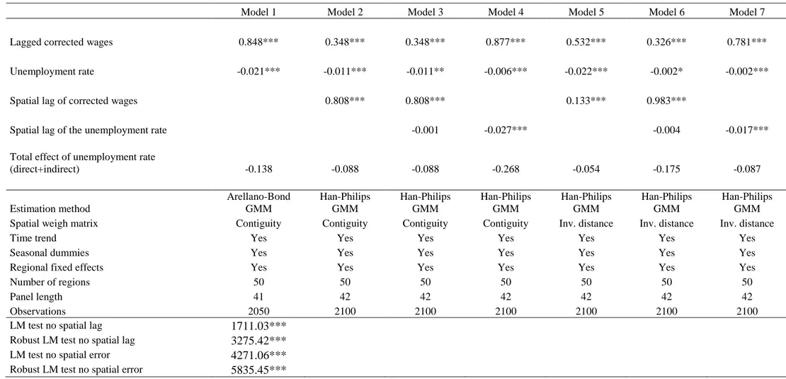
Column 1 of table 4 shows the results of estimating the dynamic specification of the wage curve (equation 4). According to the results in column 1, there is a high degree of inertia in regional wages, that is related to the peculiarities of the Spanish collective bargaining system where sectoral agreements at the regional level predominate and interregional wage differences persist (Simón et al., 2006). The elasticity of wages to unemployment is negative and statistically significant and its value is substantially lower (-0.021). However, the long run response is higher than the one found in the static model: -0.138. The inclusion of the spatial lag of corrected wages in models 2-3 and 5-6 change the picture obtained when using the static model. In particular, the spatial lag of unemployment is no longer statistically significant, while the spatial lag of corrected wages is the most relevant explanatory variable. However, this could be due to multicollinearity between the two spatially lagged variables (wages and unemployment). In fact, in models 4 and 7, neighbours’ unemployment seems to affect regional wage dynamics.
13
Table 4. Dynamic wage curve with regional spillovers
Model 1 Model 2 Model 3 Model 4 Model 5 Model 6 Model 7
Lagged corrected wages 0.848*** 0.348*** 0.348*** 0.877*** 0.532*** 0.326*** 0.781***
Unemployment rate -0.021*** -0.011*** -0.011** -0.006*** -0.022*** -0.002* -0.002***
Spatial lag of corrected wages 0.808*** 0.808*** 0.133*** 0.983***
Spatial lag of the unemployment rate -0.001 -0.027*** -0.004 -0.017***
Total effect of unemployment rate
(direct+indirect) -0.138 -0.088 -0.088 -0.268 -0.054 -0.175 -0.087 Estimation method Arellano-Bond GMM Han-Philips GMM Han-Philips GMM Han-Philips GMM Han-Philips GMM Han-Philips GMM Han-Philips GMM
Spatial weigh matrix Contiguity Contiguity Contiguity Contiguity Inv. distance Inv. distance Inv. distance
Time trend Yes Yes Yes Yes Yes Yes Yes
Seasonal dummies Yes Yes Yes Yes Yes Yes Yes
Regional fixed effects Yes Yes Yes Yes Yes Yes Yes
Number of regions 50 50 50 50 50 50 50
Panel length 41 42 42 42 42 42 42
Observations 2050 2100 2100 2100 2100 2100 2100
LM test no spatial lag 1711.03***
Robust LM test no spatial lag 3275.42***
LM test no spatial error 4271.06***
Robust LM test no spatial error 5835.45***
14
5. Final remarks
The objective of this paper was twofold: first, to obtain recent estimates of the Spanish wage curve, and second, to test whether the application of dynamic models which are augmented by a spatially weighted unemployment rate fit the Spanish data. Our results confirm the finding of a dynamic wage curve, i.e. a significant coefficient on lagged wages that, however, is far from unity, with a wage elasticity with respect to unemployment relatively small but significant (−0.02) in the short-run but more than double and close to -0.1 in the long-run. It is remarkable that the spatial lags of unemployment rate and wages are relevant to explain regional wage determination. In fact, as previously mentioned, the high relevance of neighbours’ wages implies a very low regional wage differentiation that, as previously mentioned, it is related to the peculiarities of the Spanish collective bargaining system (Simón et al., 2006).
Further research will explore whether spatial heterogeneity is also present in the relationship between unemployment in wages for Spain. According to Deller (2011), in some Southern US counties no wage curve is found, a result in line with the Harris–Todaro Model while in the Midwest and a range from Montana south to Texas along with most of the California–Nevada border region a wage curve is found. For the Spanish case, Bande et al. (2012) also advances in this direction. To analyse whether there are spatial differences in the relationship between wages and unemployment, geographically weighted regression (GWR) could be applied in this context as in Deller (2011). The main advantage of GWR is that it allows regional variations in the coefficients, but considering also the influence of neighbouring regions (Fotheringham et al., 2002). In fact, when applying this technique it is assumed that parameters of neighbouring regions are similar. So, in the estimation of the parameters for a particular region, only a subset of neighbouring regions is used. However, although there are some recent methodological proposals on how to apply geographically weighted regressions when using panel data, there is no clear consensus on how to implement them (Yu, 2010; Bruna and Yu, 2013).
6. References
Anselin, L. (1988): Spatial econometrics: Methods and models. Dordrecht: Kluwer Academic Publishers.
Anselin, L., Le Gallo, J., Jayet, H. (2006): “Spatial panel econometrics” in Matyas L, Sevestre P (eds.) The econometrics of panel
data fundamentals and recent developments in theory and practice 3rd ed. Kluwer, Dordrecht, pp. 901-969
Arellano, M, Bond, S. (1998): “Dynamic Panel Data Estimation Using DPD98 for Gauss: A Guide for Users”, mimeo.
Babecky, J., Ramos, R., Sanromá, E. (2008): “Meta-analysis on Microeconomic Wage Flexibility (Wage Curve)”, Sozialer
Fortschritt/German Social Policy Review, 57 (10-11), pp. 273-279.
Baltagi, B.H., Blien, U., Wolf, K. (2009): “New evidence on the dynamic wage curve for Western Germany: 1980-2004”, Labour
Economics, 16 (1), pp. 47-51.
Baltagi, B.H., Blien, U., Wolf, K. (2012): “A dynamic spatial panel data approach to the German wage curve”, Economic Modelling, 29 (1), pp. 12-21.
Bande, R., Fernández, M., Montuenga, V. (2012): “Wage flexibility and local labour markets: A test on the homogeneity of the wage curve in Spain”, Investigaciones Regionales, 24, pp. 175-198
Bell, B., Nickell, S., Quintini, G. (2002): “Wage equations, wage curves and all that”, Labour Economics, 9 (3), pp. 341-360. Blanchflower, D. G., Oswald, A. J. (1990): “The wage curve”, Scandinavian Journal of Economics, 92 (2), pp. 215-235.
15
Blanchflower, D. G., Oswald, A. J. (1994a): “Estimating a wage curve for Britain 1973-1990”, The Economic Journal, 104 (426), pp. 1025-1043.
Blanchflower, D. G., Oswald, A. J. (1994b): The wage curve. MIT Press: Cambridge and London.
Blanchflower, D. G., Oswald, A. J. (1995): “An Introduction to the Wage Curve”, Journal of Economic Perspectives, 9 (3), pp. 153-167.
Blanchflower, D. G., Oswald, A. J. (2005): The Wage Curve Reloaded, NBER Working Paper No. 11338
Blien, U., Dauth, W., Schank, T., Schnabel, C. (2013): “The Institutional Context of an ‘Empirical Law’: The Wage Curve under Different Regimes of Collective Bargaining”, British Journal of Industrial Relations, 51 (1), pp. 59–79.
Bruna, F., Yu, D. (2013): “Geographically Weighted Panel Regression”, XI Congreso Galego de Estatística e Investigación de Operacións, http://xisgapeio.udc.es/.
Buettner, T. (1999): “The effect of unemployment, aggregate wages, and spatial contiguity on local wages: An investigation with German district level data”, Papers in Regional Science, 78 (1), pp. 47-67.
Campbell, C. (2008): “An efficiency wage approach to reconciling the wage curve and the Phillips curve”, Labour Economics, 15 (6), pp. 1388-1415.
Campbell, C., Orszag, J. (1998): “A Model of the Wage Curve”, Economics Letters, 59 (1), pp. 119-125.
Canziani, P. (1997): The Wage Curve in Italy and Spain. Are European Wages Flexible?, Center for Economic Performance Discussion Paper 375.
Corrado, L., Fingleton, B. (2012): “Where Is The Economics In Spatial Econometrics?”, Journal of Regional Science, 52(2), pp. 210-239.
Deller, S. (2011): “Spatial heterogeneity in the wage curve”, Economics Letters, 113 (3), pp. 231-233.
Elhorst, J. P. (2000): “The mystery of regional unemployment differentials: Theoretical and empirical explanations”, Journal of
Economic Surveys, 17 (5), pp. 709-748.
Elhorst J P (2009): “Spatial Panel Data Models” in Fischer M M, Getis A (eds ) Handbook of Applied Spatial Analysis. Springer, Berlin
Elhorst, J. P., Blien, U., Wolf, K. (2007): “New evidence on the wage curve: a spatial panel approach”, International Regional
Science Review, 30, pp. 173–191.
Falk, M., Leoni, T. (2011): “Estimating the Wage Curve with Spatial Effects and Spline Functions”, Economics Bulletin, 31(1), pp. 591-604.
Fotheringham, S., Brunsdon, C., Charlton, M. (2002): Geographically Weighted Regression: the analysis of spatially varying
relationships. John Wiley & Sons, UK.
García-Mainar, I., Montuenga-Gomez, V.M. (2003): “The Spanish wage curve: 1994-1996”, Regional Studies, 37 (9), pp. 929-945. García-Mainar, I., Montuenga-Gómez, V.M. (2012): “Wage dynamics in Spain: Evidence from individual data (1994-2001)”,
Investigaciones Regionales, 24, pp. 41-56.
García-Perez, I. (2008): “La Muestra Continua de Vidas Laborales: Una guia de uso para el análisis de transiciones”, Revista de
Economía Aplicada, E-1 (vol. XVI), pp. 5-28.
Hall, R. (1972): “Turnover in the labour force”, Brookings Papers on Economic Activity, 3, pp. 706-756.
Han, C., Phillips, P. C. B. (2010): “GMM Estimation for Dynamic Panels with Fixed Effects and Strong at Unity”, Econometric
Theory, 26, pp. 119–151.
Harris, J., Todaro, M. (1970): “Migration, Unemployment and Development: A Two-Sector Analysis”, American Economic Review, 60, pp. 126-142.
Kelejian, H.H., Robinson, D.P. (1997), “Infrastructure productivity estimation and its underlying econometric specifications: A sensitivity analysis”, Papers in Regional Science, 76 (1), pp. 115-131.
Layard, R., Stephen N., Jackman R. (1991): Unemployment, Macroeconomic Performance and the Labour Market, Oxford University Press, Oxford.
Lesage, J., Pace. R. K. (2008): “Spatial Econometric Modeling of Origin-Destination Flows”, Journal of Regional Science, 48, pp. 941–967.
Longhi, S. (2012): “Job Competition and the Wage Curve”, Regional Studies, 46 (5), pp. 611-620.
Longhi, S., Nijkamp, P., Poot, J. (2006): “Spatial heterogeneity and the wage curve revisited”, Journal of Regional Science, 46 (4), pp. 707-731.
Montuenga, V., García, I., Fernández, M. (2003): “Wage flexibility: Evidence from five EU countries based on the wage curve”,
16
Montuenga, V.M., Ramos, J. M. (2005): “Reconciling the wage curve and the Phillips curve”, Journal of Economic Surveys, 19 (5), pp. 735-765.
Moulton, B. R. (1986): “Random Group Effects and the Precision of Regression Estimates”, Journal of Econometrics, 32, pp. 385-397.
Nijkamp, P., Poot, J. (2005): “The Last Word on the Wage Curve? A Meta-Analytic Assessment”, Journal of Economic Surveys, 19 (3), pp. 421-450.
Sanromá, E., Ramos, R. (2005): “Further Evidence on Disaggregated Wage Curves: The Case of Spain”, Australian Journal of
Labour Economics, 8, pp. 227-243.
Simón, H., Ramos, R., Sanromá, E. (2006): “Collective bargaining and regional wage differences in Spain: An empirical analysis”,
Applied Economics, 38 (15), pp. 1749-1760.
Yu, D. (2010): “Exploring Spatiotemporally Varying Regressed Relationships: The Geographically Weighted Panel Regression Analysis. Joint International Conference on Theory, Data Handling and Modelling in GeoSpatial Information Science. Hong Kong.