A dynamic analysis of asymmetric shocks in EU manufacturing

(1)

A DYNAMIC ANALYSIS OF ASYMMETRIC SHOCKS

IN EU MANUFACTURING

Raúl Ramos*

Grup d’Anàlisi Quantitativa Regional, Departament d’Econometria, Estadística i Economia Espanyola, Universitat de Barcelona. Av. Diagonal 690, 08034 Barcelona (Spain)

Tel. +34 +934021984 Fax: +34 +934021821 e-mail: rrlobo@eco.ub.es

Miquel Clar

Tel. +34 +934035828 Fax: +34 +934021821 e-mail: mclar@eco.ub.es

Jordi Suriñach

Tel. +34 +934021980 Fax: +34 +934021821 e-mail: surinach@eco.ub.es

ABSTRACT

Available empirical evidence regarding the degree of symmetry between European economies in the context of Monetary Unification is not conclusive. This paper offers new empirical evidence concerning this issue related to the manufacturing sector. Instead of using a static approach as most empirical studies do, we analyse the dynamic evolution of shock symmetry using a state-space model. The results show a clear reduction of asymmetries in terms of demand shocks between 1975 and 1996, with an increase in terms of supply shocks at the end of the period.

*

(2)

A DYNAMIC ANALYSIS OF ASYMMETRIC SHOCKS IN EU

MANUFACTURING

I. Introduction

Most studies analysing the possible effects of the European monetary unification (EMU) process following the Optimum Currency Areas approach conclude that the success of the EMU (when benefits overweight costs) will depend on the capacity of European economies to give more flexibility to markets —both labour and goods and services markets— and also on the degree of symmetry of future shocks (see Ramos et al., 1999). Our paper focuses on this second aspect.

The European Commission (1990) offers a very optimistic view regarding the probability of asymmetric shocks under the EMU in its report “One market, one money”. This study predicts that in the future asymmetric shocks will decrease as a consequence of two factors: the higher coordination of economic policies among participating countries and the increase in intra-industry trade and in similarities between economic structures. If this view is correct, the loss of national sovereignty on the exchange rate will have no repercussion in terms of macroeconomic adjustment capacity.

An alternative, pessimistic view is defended by Krugman (1991, 1993). Following Kenen (1969), who suggests that when a region (or a country) has a diversified territory it tends to experience less asymmetric shocks than a highly specialised territory, Krugman predicts that the complete removal of barriers to trade and the improvement of the functioning of the Single Market as a result of the EMU will lead to a higher regional concentration of industrial activity. In this sense, compared with the United States, European countries can expect higher levels of regional concentration in a near future and, as a result, more asymmetric shocks. According to Sapir (1996), however, there have only been small changes in the pattern of specialisation of European countries during the last decades.

This paper examines empirical evidence concerning the evolution of the degree of symmetry of shocks experienced by European countries and in order to identify which of both scenarios seems to predominate.

(3)

II. Asymmetric shocks in European manufacturing: evidence from the model of Bayoumi and Eichengreen (1992)

The most common way to evaluate degrees of symmetry is by calculating the correlation coefficients among the series of shocks (previously obtained using one of the available methodologies). If the values of these coefficients are high, it would be expected that the countries under study have experienced relatively symmetrical disturbances.

In this section, we will apply this approach, using the model proposed by Bayoumi and Eichengreen (1992), to obtain the series of shocks for European countries. We will focus our analysis on the manufacturing sector. This sector has felt the effects of the Single Market programme most due to its greater openness (European Commission 1990). Moreover, although the share of manufacturing in the total GDP is small, this sector is still relevant in all the European countries and manufactured goods account for a considerable share of total exports and imports in EU countries (see table 1).

TABLE 1

To distinguish shocks from responses in the evolution of production, Bayoumi and Eichengreen (1992) take as their starting point Galí’s (1992) macroeconomic model of aggregated demand and supply. From this model, predictions of the response of different macroeconomic variables to structural shocks can be made. It is also possible to identify shocks taking into account the relationships between output and price evolution. The main stilized facts that can be derived from the model are the following:

a) On the one hand, demand shocks (including shocks related to fiscal and monetary policies) have transitory effects on the production level as a result of slow adjustment of nominal variables, but permanent effects on the price level due to rigidities (King, 1993). On the other hand, supply shocks have permanent effects on output and prices.

b) Monetary shocks are transmitted to the real sector through changes in interest rates.

(4)

c) Output and prices move in the same direction in response to a demand shock and in opposite directions in response to a supply shock.

From fact a) and following Bayoumi and Eichengreen (1992), estimates of the series of demand and supply shocks can be obtained by introducing this assumption into a structural bivariate VAR model for output and prices (see appendix A). We obtained estimates of demand and supply shocks experienced by Belgium, Denmark, Finland, Germany, Greece, Ireland, Spain, Sweden and the United Kingdom1 between 1975 and 1996 through this model, using data for industrial production and industrial producer prices2. We then did the same for peripherical countries (Nordic and Mediterranean, except Portugal as data on prices were not available), using Belgium as a control for core countries and Germany, EU-11 and EU-153 as anchor areas.

We chose two different geographical areas (EU-11 and EU-15) —apart from Germany— to evaluate the degree of symmetry of shocks for both empirical and theoretical reasons4. From an empirical point of view, the comparison of the values of the correlation coefficients with the EU-11 and EU-15 gave us reference values to evaluate the advantages of a wider currency area from the analysis of European countries (without having to resort to the US). From a theoretical point of view (see Lane and Gros, 1994), the German reunification, which increased the variability of shocks in that country, has reduced the advantages of taking it as anchor area.

Prior to this, we had analysed the order of integrability of the output and price series for the considered countries and found that every considered series has a unit root. The VAR models, estimated in first differences as the null hypothesis of non cointegration, could not be rejected using the Johansen test5. As for the number of lags included in the models, we kept a homogenous identification scheme for every country. The chosen number of lags was two as it was the optimal number in most cases according to the Schwartz information criterium. The results were also satisfactory in terms of adjustment and the signs of the variables were those expected. From the residuals obtained in the estimation of these models in reduced form, we obtained the series of demand and supply shocks for every considered country applying the analytical solution of the system.

(5)

Next, we calculated the values of the correlation coefficients between these series of shocks. One disadvantage of this method, however, is that in small samples there exists the danger of accepting as true, false correlations. For this reason, we then applied the criterium to distinguish between significant and not significant correlations6 proposed by Brandner and Neuser (1992) who use as a critical value, at a 5% significance level for detrended series (as the ones considered here), 2/ n, where n is the number of available observations.

Tables 2 and 3 show the values of the correlation coefficients between the obtained series of demand and supply shocks for the considered countries. Given that the sample size is 19, the critical value proposed by Brander and Neuser is approximately ±0.46. Correlations above this value (or below for negative values) are in italics in both tables. These tables show that the correlations between the series of demand shocks are higher than those between the series of supply shocks with independence of the reference area. The average value for the period 1978 - 1996 for EU-15 is 0.44 for demand shocks and 0.42 for supply shocks. Thus, it seems that in the considered period, demand shocks were more symmetric than supply shocks.

TABLE 2

TABLE 3

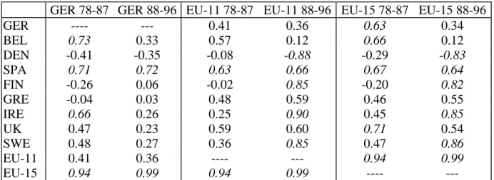
Tables 4 and 5 show the values of the correlation coefficients between the demand and supply shocks calculated for two different subperiods (1978-1987 and 1988-1996)7. In general, the correlations for demand shocks tended to decrease in the second subperiod with independence of the chosen area of reference. The average value of the correlation coefficients between EU-15 and the rest of the considered countries’ series of demand shocks was 0.46 in the first period and 0.39 in the second, while for EU-11 it was 0.46 and 0.38. The values of the correlation coefficients for supply shocks, however, increased in the second subperiod. The average value for EU-15 increased from 0.40 to 0.43 and for EU-11 from 0.35 to 0.45. This shows that in the more recent years asymmetric shocks are related to factors controllable by national governments while those related to non controllable factors tended to decrease.

(6)

TABLE 4

TABLE 5

On the other hand, the method used to analyse the evolution of the degree of symmetry of shocks (which consisted of splitting the available data into two different subperiods) may not be totally accurated: the number of different periods and the points of break are, in fact, unknown. Neither does this approach take into consideration the fact that the European economic and monetary unification process is a dynamic and gradual process. To include these two issues in our analysis, we propose a time varying coefficient model based on state-space models and estimated using the Kalman filter.

III. Methodology and results of the dynamic analysis of the degree of shock symmetry

Time varying coefficient models allow us to include in the model the possibility of changing relationships between the considered variables. Haldane and Hall (1991) were the first to use this kind of model. They used a state-space model to test to what extent movements in the Sterling Pound were associated with movements in the US Dollar or in the Deutschmark. A similar model can be used to analyse the evolution of the degree of symmetry of shocks experienced by European countries. This method was first used, to our knowledge, in the context of the European Monetary Unification process by Boone (1997) to analyse the degree of symmetry of demand and supply shocks for the entire economy. The model used was the following:



X Z



t at bt



YZ



tt; (1) t t t a a  _₁₁ ; and, (2) t t t b b  _₁₂ , (3)

where Zt represents the series of shocks in Germany, Xt the series of shocks in the

(7)

shocks in the United States). The parameters at and bt are time-varying coefficients

which allow us to assess the dynamic evolution of asymmetries.

Coefficient at is a stochastic constant which approximates all those factors that have a systemic influence on both variables. The introduction of this variable also eliminates the adverse effects of the possible omission of relevant variables in the considered relationships, specially, those factors affecting the long-run levels of both variables. The value of coefficient at summarises, then, the differences in the

average of both variables and can be interpreted as an indicator of ‘autonomous’ convergence between the considered countries.

As for bt, if

 

0



 t

t b

lim

E (meaning bt take values starting from 1 in the first

years of the considered period and ending with values near 0), then the evolution of country X has approached the area of influence of country Z in terms of shocks. If, on the contrary,

 

1



 t

t b

lim

E , then X has approached the influence area of Y (the rest of the world). In other words, in the first case shocks experienced by X and Z have tended to be more symmetric while in the second case shocks have tended to be more asymmetric.

Boone’s results, after estimating this model for the whole economy using the Kalman filter (see appendix B), provide evidence in favour of a convergence in terms of supply shocks for the core countries, and also for the peripherical countries except Greece and the UK. As for demand shocks, he finds that the distinction between core and peripherical countries is very slight, though the convergence process seems to have stopped since the mid-eighties.

Our results differ from Boone’s (1997) in two respects. First, we analyse the degree of symmetry between shocks for the manufacturing sector, not the entire economy. Second, given that a shock cannot be anticipated by definition, the series of shocks estimated following Bayoumi and Eichengreen’s (1992) method have zero mean. As a result, we must include in the specification the parameter at to

approximate the behaviour of factors affecting the long-run level of the variables as they have zero mean. Hence, in the proposed model we have imposed the restriction

at=08. Furthermore, assuming that at=0 simplifies considerably the estimation

process of the model using the Kalman filter9.

Thus, the considered model can be expressed by two equations instead of three:

(8)



X Z



_t b_t 



Y Z



_t _t; and, (4) t

t t b

b  _1 . (5)

As has been previously stated, these equations can be easily estimated for every considered country using the Kalman filter once the model is interpreted as a state-space representation: equation (4) can be understood as the measurement equation and equation (5) as the transition equation.

To obtain the estimates of the dynamic measures of the evolution of the degree of shock symmetry, we must first estimate the values of the unknown hyperparameters and solve the problem of the inicialisation of the Kalman filter. As for the estimation of the hyperparameters of the model, the only unknown values are those of the covariance matrix of the perturbations in equations (4) and (5); the rest of the hyperparameters are given by the model specification.

The unknown values of the hyperparameters were estimated by maximum likelihood. We used prediction error decomposition (Harvey, 1981 and 1984) to estimate the expression of the system likelihood function. Next, this function was maximised with respect to the estimated hyperparameters using the numeric optimisation procedure proposed by Broyden-Fletcher-Goldfarb-Shanno (BFGS). As for the treatment of the initial values of bt, we applied the method proposed by

Harvey and Phillips (1979) which consists of initialising the filter with very high values of the variance of the estimation error. This —after applying sequentially the Kalman filter equation— produces a convergence process that reduces error, giving accurate estimates of the state vector.

It is important to point out, nevertheless, that the main criticism of the application of the state-space models in Economy is related to the possible sensitivity of the results to the considered maximum likelihood procedure and the treatment of the initial values. Consequently, we also carried out a sensitivity analysis of the results following Hackl and Westlund (1996). The results were not substantially altered.

Figures 1 and 2 show the results for demand and supply shocks symmetry (the evolution of bt) between Belgium, Denmark, Finland, Greece, Ireland, Spain,

(9)

opposed to the rest of the world (USA). Table 6 also presents the OLS estimation for coefficient b for the entire period10. These estimates and the correlation coefficients presented in the previous section can be interpreted similarly, taking into account the indications made before. The conclusions derived from the analysis of these results are similar to the ones in the previous section.

TABLE 6

The dynamic analysis11 of demand shocks (figure 1), shows that nearly all the considered countries (except Denmark) present strong evidence to convergence in terms of shocks, though this convergence seems to have ceased during the last years of the studied period. With respect to Germany, the countries that show lower values of coefficient b at the end of the period (more symmetry) are Belgium and Finland while Spain, Greece, Ireland, Sweden and the United Kingdom remain at an intermediate level. Certain differences are observed, however, if we take EU-11 and EU-15 as our reference. In practically every country (except Finland) the degree of convergence is higher than it is with respect to Germany, especially in Spain, Greece, Ireland, Sweden and the UK. This could be related to the information taken into account12,13. On the other hand, the results are not surprising since demand shocks are related to differences in national macroeconomic policies —differences that have been reduced due to the greater co-ordination between EU countries. In this sense, it is important to point out that (independent of the chosen country) the trend to convergence slowed down during the last years. The relationships between demand shocks in different countries changed during the first half of the nineties due to several facts: the German reunification, the instability of the European Monetary System and the recent process of adjustment due to Maastricht requirements. However, the values of the b coefficients for the more recent years (and in particular in reference to European aggregates) show again a decreasing trend.

FIGURE 1

The case of Belgium needs mention. Although Belgium has followed a monetary policy very similar to that of Germany, it shows greater asymmetry with the European aggregates during the last years of the considered period. One

(10)

explanation could the introduction in 1992 of a convergence plan to comply with the Maastricht public deficit requirements. Moreover, although this plan was rigorously applied, conjunctural measures to achieve these desired objectives were frequently introduced. The additional adjustment these measures required with reference to other European countries could explain in part the divergence of the last years.

In Finland, the economic recession which touched bottom in 1993 strongly affected its relative position in terms of shocks. However, and thanks to an expansive monetary policy and to the consolidation of its public deficit, during the last few years it again achieved a high degree of symmetry. In Spain, the situation was similar. The reduction of the public deficit and interest rates increased the degree of symmetry in terms of demand shocks.

In Greece, the public deficit was reduced to 15% of the GDP, the Central Bank become independent and the country joined the European Monetary System which improved the process of macroeconomic convergence and greatly decreased the number of asymmetric shocks during the last years.

In Sweden, after a short period of high asymmetry related to the uncertainty of its participation in the third stage of EMU and the adoption of the convergence programme in 1994, the degree of symmetry also improved during the last years of the considered period.

On the contrary, the increase in asymmetry in Denmark and the UK can be related to their lack of political willingness to take part in the final stage of EMU. The increase of the b coefficient for Ireland with respect to EU-15, but not EU-11, can be related to this fact, given the relevance of the relationships between Ireland and the UK.

As for supply shocks (figure 2), the results also show a trend to convergence in reference to EU-11 and EU-15 during practically the entire period. The convergence process in terms of shocks symmetry also accelerated from the middle of eighties, which can be related to the effects of the Single Act. The results obtained taking Germany as reference are very different, however. Without doubt, this can be related to the impact of the German reunification as can be appreciated from the results for Finland and Sweden. For these two countries, the values of coefficient b are lower with respect to EU-11 or EU-15 than with respect to Germany from the beginning of the nineties. In the case of Denmark, the convergence slowed down in the early nineties with independence of the country of reference. Both the lower

(11)

symmetry of Finland and Sweden with respect to Germany and the exceptional case of Denmark are related to the evolution of manufacturing productivity during those years (see figure 3).

FIGURE 2

FIGURE 3

During the early nineties Finland and Sweden underwent a profound process of industrial reallocation. The sectors with higher technological components and higher export capacity were favoured and promoted in detriment of the rest. This process of reform, supported by direct foreign investment, together with labour market reforms, increased the productivity of the manufacturing sector (see figure 3) through positive supply shocks. Because this situation was similar in most of the considered countries except Germany, both EU-15 and EU-11 reflect this fact.

The situation of Denmark was, however, very different. Until 1994, the Danish government did not readdress its industrial policy. Until then the Danish industrial policy was practically inexistent —a fact that produced little concern during the expansive periods of the eighties but became a serious drawback during the crisis. The first things the Danish government did were to create a Ministry to co-ordinate the sectoral-specific measures addressed to firms and to invest in infrastructures. The results of these actions seem to have changed the negative trend in terms of supply shocks asymmetry to a more positive situation.

IV. Conclusions

The results presented in this paper suggest that demand shocks experienced by European countries were more symmetric in the last years of the studied period, especially in reference to the EU-11 and EU-15 aggregates. In this sense, it is important to point out that the situation worsened with respect to Germany, possibly as a consequence of German reunification. As for supply shocks, the degree of symmetry is higher now than in the mid seventies, but especially since the mid eighties (Single Act, Single Market Programme).

(12)

As a consequence, and taking into account that it is not possible to discard the scenario proposed in the context of Economic Geography, the results show a clear predominance of the optimistic scenario predicted by the European Commission. The dynamic analysis of the convergence of demand and supply shocks has also allowed us to identify the period of the mid eighties as the period of greater convergence. During the latter years, however, shocks tended to be more asymmetric again. One possible explanation could be an increase in productive specialisation in the considered countries as a result of the effects of the Single Market Programme. Reliable data to contrast this hypothesis are not yet available.

Acknowledgements

We would like to thank T. Bayoumi and B. Eichengreen, who kindly provided us with their TSP programs to calculate the series of shocks. Support from the Spanish Ministry of Education and the ERFD through the project 2FD97-1004-C03-01 and the Plan Nacional de I+D APC1999-0081 is gratefully acknowledged. Last, but not least, we are also grateful to comments made by E. López-Bazo and E. Pons. Of course, all remaining errors are our own.

(13)

Notes

1.

Other countries such as Austria, France, Netherlands and Luxembourg have not been considered due to the reduced number of available observations for the index of industrial prices, which would affect the validity of the results of the specified VAR model. In any case, the number and characteristics of the considered countries are representative enough to obtain valid conclusions about the evolution of the degree of symmetry of shocks in EMU.

2.

Indicators of Industrial Activity, OECD, 1998. 3.

To approximate the evolution of the industrial production and industrial producer prices of EU-15 and EU-11, we have constructed two composed indexes using disaggregated data at a national level and applying the same weights as the OECD for the year 1990. It is important to point out that, although there were some problems related to the lack of statistical information for the entire considered period, both aggregated indicators incorporate information about all member countries. To obtain the series of demand and supply shocks, the applied methodology has been the same for any individual country.

4.

This is a difference with most empirical works where only Germany is considered as the anchor area for shock asymmetry.

5.

The only exception was Sweden, but the model was also estimated in differences to keep homogeneity.

6.

As the size of this test is reduced, the conclusions derived from the analysis are only orientative and they will be extended in the next section.

7.

The critical values following Brandner and Neuser (1992) are, respectively, 0.63 and 0.66. 8.

Hall et al. (1992) reason similarly when they impose this assumption to analyse the relationships between European countries in terms of inflation evolution.

9.

It reduces the number of hyperparameters to be estimated and the treatment of initial values, so one can expect that the obtained estimates would be more robust than in the previous specification. 10.

To compare the time-varying with the OLS models, we calculated the ratio between the sum of squares of the residuals (SSRvar/SSRols). In all cases, the results were below 1, so the time-varying model seems to fit the data better than the OLS model.

11.

It is important to point out that the analysis of symmetry could be affected by the magnitud of the variance of the residuals respect to the variance of the reference country shocks (the relative importance of the anchor area). In nearly all cases, the estimated variance of the residuals is much lower than the variance of Zt.

12.

The existence of missing data in some of the series used to elaborate the European aggregates could partially explain these results.

13.

This fact could also explain the negative values of the b coefficient in those cases where the European aggregates are taken as reference areas. One possible solution would be to restrict the estimation of the coefficient to values between 0 and 1, but we discarded this solution in order to maintain the homogeneity with the results for Germany.

14.

It is important to point out that only indirect effects are considered as we are using data for West Germany.

(14)

References

Anderson, B.and J. Moore (1979) Optimal Filtering, Prentice-Hall, Englewoods Cliffs.

Ansley, C. and R. Kohn (1989) Filtering and smoothing in state-space models with partially diffuse initial conditions, Journal of Time Series Analysis, 11, 275-93.

Bayoumi, T. and B. Eichengreen (1992) Shocking Aspects of European Monetary Unification, NBER WP 3949.

Bayoumi, T. and B. Eichengreen (1996) Operationalizing the Theory of Optimum Currency Areas, CEPR Discussion Paper 1484.

Boone, L. (1997) Symetrie des chocs en Union Europeenne: Un analyse dynamique, Economie Internationale, 70, 7-34.

Brandner, P. and K. Neusser (1992) Business cycles in open economies: Stylized facts for Austria and Germany, Weltwirtchaftliches Archiv, 128, 67-87.

European Commission (1990) One market, one money, European Economy, 44.

Cuthberson, K., S. Hall and M. Taylor (1992) Applied Econometric Techniques, Phillip Allan, New York.

de Grauwe, P. (1997) The Economics of Monetary Integration. (Third Edition) Oxford University Press, Oxford.

de Jong, P. (1991) The diffuse Kalman filter, The Annals of Statistics, 19, 1073-83.

Galí, J. (1992) How well does the IS-LM model fit Postwar U.S. data?, Quarterly Journal of Economics, 107, 709-38.

Hackl, P. and A. Westlund (1996) Demand for international telecomunication: Time-varying price elasticity, Journal of Econometrics, 70, 243-60.

Haldane, A. and S. Hall (1991) The Sterling's relationship with the Dollar and the Deustchmark: 1976-92, Economic Journal, 101, 436-443.

Hall, S., D. Robertson and M. Wickens (1992) Measuring convergence of the EC economies, The Manchester School of Economic and Social Studies, 60, 99-111.

Harvey, A. (1981) The Econometric Analysis of Time Series, Deddington, Oxford.

Harvey, A. (1982) The Kalman filter and its applications in Econometrics and time series analysis, Methods of Operational Research, 44, 3-18.

Harvey, A. (1984) Dynamic models, the prediction error decomposition and state space models, in D. Hendry and K. Wallis (eds.) Econometrics and Quantitative Economics, Basil Blackwell, Oxford.

Harvey, A. (1987) Applications of the Kalman filter in Econometrics, in T. Bewley (ed.) Advances in Econometrics: Fifth World Congress, Econometric Society Monograph 13, Cambridge University Press, Cambridge.

Harvey, A. (1989) Forecasting, Structural Time Series Models and the Kalman Filter, Cambridge University Press, Cambridge.

Harvey, A. and G. Phillips (1979) Maximum likelihood estimation of regression models with autoregressive-moving average disturbances, Biometrika, 66, 69-58.

(15)

Kalman, R. (1960) A new approach to linear filtering and prediction problems, Transactions ASME, Journal of Basic Engineering, 82, 35-45.

Kalman, R. and R. Bucy (1961) New results in linear filtering and prediction theory, Transactions ASME, Journal of Basic Engineering, 83, 95-108.

Kenen, P. (1969) The theory of optimum currency: An eclectic view, in R. Mundell and A. Swoboda (eds.) Monetary Problems of the International Economy, Chicago University Press, Chicago. King, R. (1993) Will the new Keynesian Macroeconomics resurrect the IS-LM model, Journal of

Economic Perspectives, 7, 67-82.

Kitagawa, G. and W. Gersch (1984) ‘A smoothness prior-state space modeling of time series with trend and seasonality’, Journal of the American Statistical Association, 82, 1032-63.

Krugman, P. (1991) Geography and Trade, The MIT Press, Cambridge (Massachussets)

Krugman, P. (1993) Lessons of Massachussets for EMU, in F. Torres and F. Giavazzi (eds.) Adjustment and Growth in the European Monetary Union, Cambridge University Press, Oxford.

Lane, T. and D. Gros (1994) Symmetry versus asymmetry in a fixed exchange rate system, Kredit und Kapital, 27, 43-66.

Ramos, R., M. Clar and J. Suriñach (1999) Specialisation in Europe and asymmetric shocks: potential risks of EMU in M. M. Fischer and P. Nijkamp (eds.) Spatial Dynamics of European Integration. Political and Regional Issues at the Turn of the Millenium, Springer-Verlag, Berlin, pp. 63-93.

Rosenberg, B. (1973) Random coefficient models: The analysis of a cross section of Time Series by stochastically convergent parameter regression, Annals of Economic and Social Measurement,

2, 399-427.

Sapir, A. (1996) The effects of Europe’s internal market programme on production and trade: A first assessment, Weltwirtschaftliches Archiv, 132, 457-75.

(16)

Appendix A: The model of Bayoumi and Eichengreen (1992)

The starting point of the system is the following:

      st dt i i i i i t t a a a a P Y   0 21 22 12 11 , (6)

where Yt and Pt represent, respectively, changes in the logarithm of output and

prices at time t, dt and st represent supply and demand shocks and akji represent each

of the element of the impulse-response function to shocks.

The identification restriction is based on the previously stated assumption about the effects of the shocks. As output data is in first differences, this implies that cumulative effects of demand shocks on output must be zero:

   0 11 0 i i a . (7)

The model defined by equations (6) and (7) also implies that the bivariate endogenous vector can be explained by lagged values of every variable. If Bi

represents the value of model coefficients, the model to be estimated is the following:                 pt yt t t t t t t e e P Y B P Y B P Y ... 2 2 2 1 1 1 , (8)

where eyt and ept are the residuals of every VAR equation. Equation (8) can be also

expressed as:            pt yt pt yt t t e e L B L B I e e L B I P Y ...) ) ( ) ( ( )) ( ( 1 2 , (9)

(17)

      pt yt i i i i i t t e e d d d d P Y 0 21 22 12 11 . (10)

Putting together equations (6) and (10):

        st dt i i i i i i pt yt i i i i i a a a a L e e d d d d   0 21 22 12 11 0 21 22 12 11 , (11)

a matrix, denoted by c, can be found that relates demand and supply shocks with the residuals from the VAR model.

           st dt st dt i i i i i i i i i i i pt yt c a a a a L d d d d e e     0 21 22 12 11 1 0 21 22 12 11 . (12)

From (12) it seems clear that in the 2x2 considered model, four restrictions are needed to define uniquely the four elements of matrix c. Two of these restrictions are simple normalisations that define the variances of shocks dt and st. The usual

convention in VAR models consists of imposing the two variances equal to one, which together with the assumption of orthogonality define the third restriction

c’c=, where  is the covariance matrix of the residuals ey y ep. The final restriction

that permits matrix c to be uniquely defined comes from Economic Theory and has been previously defined in equation (7). In terms of the model introducing (7) in (12), it follows that:     . . . 0 22 21 12 11 0 21 22 12 11 c c c c d d d d i i i i i , (13)

and the resolution of this system permits us to estimate the series of demand and supply shocks from residuals of the estimated VAR.

(18)

Appendix B. State-space models and the Kalman filter

Many conventional dynamic models can be easily written in a state-space form. The state-space form offers a more flexible way of treating the identification and estimation of dynamic models and this is the reason why state-space models have been widely used by economists in the last years (see Harvey, 1982 and 1987).

A state space model consists of two equations: the measurement equation and the transition equation. The measurement equation relates a nx1 vector Yt with t, a mx1

vector of unobservable variables through the following expression:

t t t t t Z d Y     , (14)

where Zt is a nxm matrix, dt is a nx1 vector of exogenous variables and t is a nx1 vector

of serially uncorrelated disturbances with zero mean and known covariance matrix: Ht:

t ~ Niid(0nx1,Hnxn).

Although, in general, the elements of t are not observable, it is assumed that

their behaviour can be estimated by a first-order Markov process:

t t t t t t T  c R     _1   , (15)

where Tt is a mxm matrix, ct is an mx1 vector of exogenous variables which influence

t, Rt is an mxg matrix and t is a gx1 vector of serially uncorrelated disturbances with

zero mean and covariance matrix Qt: t ~ Niid(0mx1, Qmxm).

Equation (15) is known as a transition equation or system equation and together with equation (14) they form the state space model.

Zt, dt, Ht, Tt, ct, Rt and Qt are known as hyperparameters and the specification of

the state-space model is completed by two further assumptions concerning the initial state vector values and the covariance matrix of the disturbances:

 

; var ; 0 0 0 0 P a E     (16)





0 s,t 1,...,T; E _t_s   (17)

(19)









0 1,..., . ; ,..., 1 0 0 0 T t E T t E t t          (18)

The Kalman filter is a recursive procedure for computing the optimal estimates of the state vector at time t, using the information available at time t-1, and updating these estimates as additional information becomes available. This filter, originally proposed by Kalman (1960) and Kalman and Bucy (1961), is proposed by two sets of equations which are applied sequentially:

Stage One: First we must obtain the optimal predictor of the next observation of the state vector (time t) using all the available information (until t-1). Let at-1 denote the

optimal estimator of t-1 based on the observations up to and including Yt-1, the mxm

estimation error covariance matrix Pt-1 associated to this estimator is given by:



 





₁ ₁ ₁ ₁ '



1       t  t  t  t t E a a P   . (19)

Once at-1 and Pt-1 are known, the optimal estimator of t restricted to these

values is given by:



_t _t

 

_t _t _t _t _t



_t _t _t t t t t a E a E T a c R T a c a _/ _₁  / _₁   / _₁   _₁     _₁ , (20)

with a covariance matrix of the estimation errors equals to:



 





a /a ₁ a /a ₁ '



T P T '+R Q R '

E =

Pt/t-1 t  t t t  t t  t t-1 t t t t . (21)

Stage Two: Next we must update the predictor of t, at/t-1 incorporating the

additional information available at time t:



t t t t t



t t t t t t t t t a a P Z F Y Z a d a   _  _       / _1 1 1 / 1 / / ' ; (22) 1 / 1 1 / 1 / '           _t _t _t _t _t _t _t _t _t t P P Z F Z P P ; (23) t t t t t t Z P Z H F   _/ _₁ ' . (24)

(20)

The Kalman filter equations can only be applied if the initial values of the state vector a0, its associated estimation error covariance matrix P0 and the values of

the hyperparameters are known. If these values are not known, they must be estimated before applying the Kalman filter. In this sense, the classical theory of maximum likelihood estimation can be adapted to obtain estimates of the hyperparameters. The procedure is summarised in the following figure:

FIGURE 4

To solve the problem of the initialisation of the Kalman filter, two procedures exist depending whether the state vector is stationary or not. A state-space model is stationary if the given values of the matrix Tt in equation (15) are within the unit circle

and there are enough observations of the considered system to affirm that the model has reached stationarity. In this situation, the initial values of the state vector can be estimated from the unconditional mean of the considered process. Following Harvey (1984), these values can be obtained using the first available m observations to estimate the equation (14) using OLS and, next, initialising the Kalman filter at time m+1. The main disadvantage of this method is that when the number of available observations is small, the degrees of freedom of the system is very limited. Another alternative consists of considering the initial values as unknown hyperparameters and estimating them by maximum likelihood (Rosenberg, 1973).

However, when the model is not stationary, the initial conditions are not well defined and the previous solutions can not be applied. The most usual solution in this case consists of treating the initial conditions as diffuse, introducing complementary equations to the usual Kalman filter. In the literature, different ways of introducing these equations have been proposed (for example, Harvey and Phillips, 1979; Anderson and Moore, 1979; Kitagawa and Gersch, 1984; Ansley and Kohn, 1989, de Jong, 1991), but none are completely satisfactory.

(21)

Tables

Table 1. Relative weight of the industrial sector on total GDP and relative weights of

exports and imports in manufactured products on total trade in 1996 (in percentage)

Country GDPm/GDP Xm/X Mm/M Country GDPm/GDP Xm/X Mm/M Germany 30.6 88.37 73.40 Netherlands 27.1 64.87 74.63 Austria 30.5 96.89 83.66 Ireland 40.2 76.96 78.31 Belgium 28.5 80.91 75.21 Italy 31.6 90.50 69.80 Denmark 24.3 63.92 77.84 Luxembourg 24.0 80.91 75.21 Spain 31.7 79.76 73.76 Portugal 33.4 86.57 75.43

Finland 31.4 85.92 74.31 United Kingdom 27.5 85.57 80.52

France 26.0 81.42 78.36 Sweden 27.5 81.79 80.65

Greece 20.0 60.54 73.87

EU-15 29.1 80.33 76.33 EU-11 29.7 87.34 82.79

GDPm= Manufacturing GDP; Xm: Exports of manufactured products; Mm: Imports of manufactured products.

Source: National Accounts 1998, Trade by Commodities, Series C, 1998, OECD.

Table 2. Correlations between demand shocks series 1978-1996

GER BEL DEN SPA FIN GRE IRE UK SWE EU-11 EU-15

GER 1.00 0.76 -0.57 0.62 0.65 0.48 0.51 0.57 0.23 0.65 0.73 BEL 1.00 -0.55 0.49 0.52 0.24 0.54 0.66 0.25 0.54 0.59 DEN 1.00 -0.56 -0.57 -0.10 -0.42 -0.48 -0.26 -0.29 -0.36 SPA 1.00 0.67 0.36 0.58 0.49 0.33 0.63 0.68 FIN 1.00 0.27 0.47 0.47 0.26 0.34 0.38 GRE 1.00 0.25 0.17 -0.07 0.56 0.44 IRE 1.00 0.47 0.48 0.63 0.65 UK 1.00 0.34 0.51 0.56 SWE 1.00 0.32 0.31 EU-11 1.00 0.96 EU-15 1.00 Aver. 0.46 0.40 -0.42 0.43 0.35 0.26 0.42 0.38 0.22 0.48 0.49

(22)

Table 3. Correlations between supply shocks series 1978-1996

GER BEL DEN SPA FIN GRE IRE UK SWE EU-11 EU-15

GER 1.00 0.50 -0.38 0.71 0.01 0.01 0.42 0.35 0.37 0.38 0.47 BEL 1.00 -0.14 0.24 -0.17 -0.13 0.45 0.24 0.32 0.33 0.37 DEN 1.00 -0.52 -0.46 -0.35 -0.51 -0.14 -0.61 -0.50 -0.57 SPA 1.00 0.32 0.41 0.48 0.35 0.50 0.62 0.63 FIN 1.00 0.45 0.51 0.27 0.52 0.54 0.49 GRE 1.00 0.27 0.62 0.38 0.52 0.50 IRE 1.00 0.55 0.62 0.58 0.64 UK 1.00 0.52 0.56 0.62 SWE 1.00 0.56 0.63 EU-11 1.00 0.96 EU-15 1.00 Aver. 0.48 0.41 0.39 0.40 0.43 0.19 0.50 0.41 0.01 0.51 0.51

Table 4. Correlations among demand shocks by subperiods

GER 78-87 GER 88-96 EU-11 78-87 EU-11 88-96 EU-15 78-87 EU-15 88-96

GER --- --- 0.69 0.54 0.76 0.66 BEL 0.77 0.73 0.55 0.51 0.62 0.57 DEN -0.63 -0.35 -0.21 -0.30 -0.36 -0.30 SPA 0.62 0.71 0.72 0.63 0.77 0.62 FIN 0.80 0.36 0.55 -0.04 0.64 -0.03 GRE 0.37 0.63 0.65 0.34 0.47 0.34 IRE 0.70 0.23 0.81 0.57 0.82 0.51 UK 0.72 0.40 0.48 0.54 0.51 0.60 SWE 0.01 0.41 -0.13 0.63 -0.05 0.56 EU-11 0.69 0.54 --- --- 0.96 0.97 EU-15 0.76 0.66 0.96 0.97 ---- ---

Table 5. Correlations among supply shocks by subperiods

GER 78-87 GER 88-96 EU-11 78-87 EU-11 88-96 EU-15 78-87 EU-15 88-96

GER ---- --- 0.41 0.36 0.63 0.34 BEL 0.73 0.33 0.57 0.12 0.66 0.12 DEN -0.41 -0.35 -0.08 -0.88 -0.29 -0.83 SPA 0.71 0.72 0.63 0.66 0.67 0.64 FIN -0.26 0.06 -0.02 0.85 -0.20 0.82 GRE -0.04 0.03 0.48 0.59 0.46 0.55 IRE 0.66 0.26 0.25 0.90 0.45 0.85 UK 0.47 0.23 0.59 0.60 0.71 0.54 SWE 0.48 0.27 0.36 0.85 0.47 0.86 EU-11 0.41 0.36 ---- --- 0.94 0.99 EU-15 0.94 0.99 0.94 0.99 ---- ---

(23)

Table 6. Values of b coefficient for the whole sample

Demand Supply

Germany EU-11 EU-15 Germany EU-11 EU-15

Belgium 0.25 0.25 0.19 0.16 0.37 0.26 Denmark 0.78 0.70 0.79 0.57 0.65 0.80 España 0.34 0.06 0.04 0.05 0.22 0.09 Finland 0.19 0.29 0.24 0.44 0.13 -0.12 Greece 0.43 0.17 0.41 0.79 0.33 0.28 Ireland 0.51 0.32 0.30 0.36 0.27 0.09 United Kingdom 0.35 0.22 0.16 0.80 0.57 0.53 Sweden 0.41 0.11 0.17 0.43 0.29 0.12

(24)

Figure 1. Convergence of demand shocks respect to Germany, UE-11 and UE-15 in relative terms of the rest of the world Belgium -0,2 -0,1 0 0,1 0,2 0,3 0,4 0,5 0,6 0,7 0,8 19781979 19801981198219831984 19851986198719881989 19901991199219931994 19951996 Germany EU-11 EU-15 Denmark 0 0,2 0,4 0,6 0,8 1 1,2 1,4 1,6 1978197919801981 1982198319841985198619871988198919901991 19921993199419951996 Germany EU-11 EU-15 Finland -1 -0,8 -0,6 -0,4 -0,2 0 0,2 0,4 197819791980198119821983198419851986198719881989 1990199119921993199419951996 Germany EU-11 EU-15 Greece -0,2 -0,1 0 0,1 0,2 0,3 0,4 0,5 0,6 0,7 0,8 19781979198019811982198319841985 198619871988198919901991 19921993199419951996 Germany EU-11 EU-15 Ireland -0,2 -0,1 0 0,1 0,2 0,3 0,4 0,5 0,6 0,7 0,8 19781979198019811982 1983198419851986 1987198819891990 19911992199319941995 1996 Germany EU-11 EU-15 Spain -0,6 -0,4 -0,2 0 0,2 0,4 0,6 19781979198019811982 198319841985198619871988 1989199019911992199319941995 1996 Germany EU-11 EU-15 Sweden -0,6 -0,4 -0,2 0 0,2 0,4 0,6 0,8 19781979198019811982 19831984198519861987 19881989199019911992 1993199419951996 Germany EU-11 EU-15 United Kingdom -0,4 -0,3 -0,2 -0,1 0 0,1 0,2 0,3 0,4 0,5 0,6 197819791980198119821983 19841985198619871988198919901991 19921993199419951996 Germany EU-11 EU-15

(25)

Figure 2. Convergence of supply shocks in respect to Germany, EU-11 and EU-15 in relative terms of the rest of the world 1978-1996 Belgium -0,4 -0,3 -0,2 -0,1 0 0,1 0,2 0,3 0,4 0,5 0,6 197819791980198119821983 198419851986198719881989 199019911992199319941995 1996 Germany EU-11 EU-15 Denmark -0,2 0 0,2 0,4 0,6 0,8 1 1978197919801981198219831984198519861987198819891990 199119921993199419951996 Germany EU-11 EU-15 Finland -1 -0,8 -0,6 -0,4 -0,2 0 0,2 0,4 0,6 1978197919801981 1982198319841985 19861987198819891990 19911992199319941995 1996 Germany EU-11 EU-15 Greece -0,2 0 0,2 0,4 0,6 0,8 1 1,2 197819791980198119821983 198419851986198719881989 199019911992199319941995 1996 Germany EU-11 EU-15 Ireland 0 0,1 0,2 0,3 0,4 0,5 0,6 0,7 19781979 198019811982198319841985 19861987198819891990 199119921993199419951996 Germany EU-11 EU-15 Spain -0,3 -0,2 -0,1 0 0,1 0,2 0,3 0,4 1978197919801981198219831984198519861987198819891990199119921993199419951996 Germany EU-11 EU-15 Sweden -0,6 -0,4 -0,2 0 0,2 0,4 0,6 1978197919801981198219831984198519861987198819891990199119921993199419951996 Germany EU-11 EU-15 United Kingdom 0 0,2 0,4 0,6 0,8 1 1,2 19781979 1980198119821983 1984198519861987 1988198919901991 1992199319941995 1996 Germany EU-11 EU-15

(26)

Figure 3. Evolution of manufacturing productivity (Real GAV per worker 1987=100)

Source: Own elaboration from Historical Statistics, 1998, OECD.

75,0 85,0 95,0 105,0 115,0 1981 1982 1983 1984 1985 1986 1987 1988 1989 1990 1991 1992 Germany Denmark Finland Sweden EU-15

(27)

Figure 4. Maximum likelihood estimation procedure of the unknown hyperparameters

Adapted from Cuthberson et al. (1992, p. 214)

Initial values Z0, T0, H0, R0 and Q0

Kalman filter equations to obtain the innovations

The prediction error decomposition (Harvey, 1984) permits to obtain the value of the likelihood function conditioned to

Z0, T0, H0, R0 and Q0

Is the value of the likelihood function a maximum?