SOLUTION FOR THE SCHR ¨ODINGER EQUATION WITH POLYNOMIAL POTENTIAL
S. ALBEVERIO AND S. MAZZUCCHI
Abstract. A functional integral representation for the weak so-lution of the Schr¨odinger equation with a polynomially growing potential is proposed in terms of an analytically continued Wiener integral. The asymptotic expansion in powers of the coupling con-stant λ of the matrix elements of the Schr¨odinger group is studied and its Borel summability is proved.
Key words: Feynman path integrals, Schr¨odinger equation, ana-lytic continuation of Wiener integrals, polynomial potential, as-ymptotic expansions.
AMS classification : 35C15, 35Q40, 35C20, 34M30, 28C20, 47D06, 35B60.
1. Introduction The Schr¨odinger equation
! i!∂
∂tψ = − !2
2m∆ψ + V ψ
ψ(0, x) = ψ0(x) (1)
with a polynomial potential V of the form V (x) = λ|x|2M and the
asymptotic behaviour of its solution in some limiting situation (for instance when λ → 0 or ! → 0, or t → 0) is a largely studied topic [10, 28, 11, 9]. Particularly interesting is the study of a possible functional integral representation, in the spirit of Feynman path integrals.
During the last four decades, rigorous mathematical definitions of the heuristic Feynman path integrals have been given by means of different methods, and the properties of these rigorous integrals have been studied. let us mention here only three of them, namely the one using the analytic continuation of Wiener integrals [12, 13], the one provided by infinite dimensional oscillatory integrals [1, 23] and the one using white noise calculus [17] (see also the references given in [1, 23] to other approaches). The main problem which is common to all the existing approaches is the restriction on the class of potentials
V which can be handled. For most results one has to impose that V has at most quadratic growth at infinity. There are two exceptions to this restriction, the one of potentials which are Laplace transform of measures (like exponential potentials, see [1, 17] and references therein) and quartic potentials [4, 8, 22].
A difficulty in the study of equation (1) with a polynomial potential is the non regular behaviour of the solution. Indeed in [31] it has been shown that for superquadratic potentials the fundamental solution of (1) is nowhere of class C1.
In [4, 8, 22] an infinite dimensional oscillatory integral representa-tion for the weak solurepresenta-tion of the Schr¨odinger equarepresenta-tion, i.e. the matrix element of the Schr¨odinger group, has been presented and studied in the case where the potential has precisely a quartic growth at infinity. The present paper generalizes partially these results to polynomial potentials with higher growth at infinity. For a dense set of vec-tors φ, ψ ∈ L2(Rd), we define an analytically continued Wiener
in-tegral Ii
t(φ, ψ) (equation (28)) which realizes rigorously the Feynman
path integral representing the corresponding ”matrix elements” of the Schr¨odinger group $φ, e−!iHtψ% and prove that it solves the Schr¨odinger
equation in a weak sense (theorem 8). The relation between the func-tional integral Ii
t(φ, ψ) and the matrix elements $φ, e− i
!Htψ% is
inves-tigated in details. In particular we prove that these quantities are asymptotically equivalent both as t → 0 and as λ → 0. The asymp-totic expansion in powers of λ of $φ, e−i
!Htψ% is studied and its Borel
summability is proved. This result allows one to recover the matrix elements of the Schr¨odinger group from the asymptotic expansion in powers of λ of the functional integral Ii
t(φ, ψ), which in this sense can be
recognized as an asymptotic weak solution of the Schr¨odinger equation. The paper is organized as follows. In section 2 the analyticity prop-erties of the spectrum of the anharmonic oscillator Hamiltonian H and of the matrix elements $φ, e−!iHtψ% of the Schr¨odinger group are
stud-ied. In section 3 the Borel summability of the asymptotic expansion in powers of the coupling constant λ (Dyson expansion) of the quantities $φ, e−!iHtψ% is proved. Section 4 studies the definition and the
proper-ties of the functional integral Ii
t(φ, ψ), while section 5 investigates its
relations with the matrix elements of the Schr¨odinger group and their asymptotic equivalence.
2. The Schr¨odinger equation with polynomial potential Let us consider the quantum anharmonic oscillator Hamiltonian with polynomial potential on L2(Rd), that is the operator defined on the
vectors φ ∈ C∞ 0 (Rd) by Hφ(x) = −! 2 2 ∆ψ(x) + λV2M(x)ψ(x), x ∈ R d, (2)
where λ ∈ R is a real positive “coupling” constant, V2M is a
posi-tive homogeneous 2M -order polynomial, and ! is the reduced Planck’s constant (the mass of the particle is set equal to 1 for simplicity). In the following, in order to simplify some notations, we shall put V2M(x) := |x|2M, but all our results are also valid in the more
gen-eral case as they depend only on the positivity and the homogeneity properties of the potential V2M.
H is essentially self-adjoint on C∞
0 (Rd) (see [26], theorem X.28). Its
closure, denoted again by H, has the following domain: D(H) = D(∆) ∩ D(|x|2M) = {φ ∈ L2(Rd) : " |x|4M|φ(x)|2dx < ∞, " |p|4| ˆφ(p)|2dp < ∞}, where ˆφ denotes the Fourier transform of φ. It is well known that H is a positive operator with a pure point spectrum {En} ⊂ R+. Therefore
−H generates an analytic contraction semigroup, P (z) : L2(Rd) →
L2(Rd), P (z) = e−Hz, with z being a complex parameter with positive
real part.
In the case where z is purely imaginary of the form z = !it, t ∈ R, one
obtains a one parameter group of unitary operators U (t) := e−!iHt, i.e.
the Schr¨odinger group. Given a vector ψ0 ∈ L2(Rd), the vector ψ(t) :=
U (t)ψ0 belongs to D(H) and it satisfies the Schr¨odinger equation:
i!∂
∂tψ(t) = Hψ(t). (3)
The particular form of the potential allows one to prove a scaling property for the eigenvalues {En} of the operator H as well as their
analyticity as a function of the coupling constant λ on a suitable region of a Riemann surface. The present lemma is taken from [28], which presents a detailed study of this problem, also in more general cases. Lemma 1. Let En(λ) denote the n−th eigenvalue of the Hamiltonian
(2). Then for λ, α > 0 one has
En(λ) = α−1En(λαM +1) = . (4) In particular En(λ) = λ 1 M +1E n(1) (5)
Proof: Let us consider, for any α ∈ R+, the unitary operator V (α) : L2(Rd) → L2(Rd) given on vectors φ ∈ S(Rd) by:
V (α)φ(x) = α1/4φ(α1/2x), x ∈ Rd. (6) It it simple to verify that V (α) leaves D(−∆) and D(|x|2M) invariant
and V (α)x2MV (α)−1 = αMx2M, V (α)∆V (α)−1 = α−1∆. It follows that V (α)HV (α)−1 = α−1#− ! 2 2 ∆ + α M +1λx2M$.
In particular, by taking α = λ−1/(M+1) one has
V (λ−1/(M+1))HV (λ−1/(M+1))−1 = λ1/(M +1)#−!
2
2 ∆ + x
2M$. (7)
As for any α ∈ R+, the operator V (α)HV (α)−1 has the same spectrum
of H, from equation (7) one easily deduces equation (5)
Remark 1. By analytic continuation, relation (5) allows to extends En(λ) to all complex values of λ belonging to a Riemann surface. In
particular, the function En is many-sheeted and has a (M + 1)-st order
branch point at λ = 0.
Let us consider now the matrix elements of the evolution operator U (t) = e−i
!Ht, i.e. the inner products $φ, U(t)ψ%, with φ, ψ ∈ L2(Rd).
Let us consider also the function f : R+ → C of the coupling constant
λ (present in H, hence in U (t)) defined by
f (λ) := $φ, U(t)ψ%, λ ∈ R, λ > 0. (8) Let us denote by Dθ1,θ2 the sector of of the Riemann surface ˜C of the
logarithm defined by:
Dθ1,θ2 := {z ∈ C, z = ρe iφ
: ρ > 0, φ ∈ (θ1, θ2)}.
Let us consider the dense subset of L2(Rd) made of finite linear
combinations of vectors of the form
φ(x) = P (x)e−σ2|x|2, x ∈ Rd (9) with P being any polynomial with complex coefficients and σ2 ∈ C a
complex constant with positive real part (that these vectors are dense in L2(Rd) follows from the known fact that the finite linear combinations
Theorem 1. Let φ, ψ ∈ S(Rd) ⊂ L2(Rd), such that the functions
¯
φ, ψ ∈ S(Rd) are of the form (9), with σ2 ∈ C, σ2 = |σ2|eiδ, δ ∈ R
such that there exist an * > 0 with
cos(δ + α) > *, ∀α ∈#0,M − 1 M + 1π
$
, (10)
(This is the case for instance if δ = −π2(M +1)M −1 ). Then the function
f : R+ → C defined by (8) can be extended to an analytic function on
the sector D−(M−1)π,0 of the Riemann surface ˜C of the logarithm.
Proof: Let us denote by {En(λ)}, resp. {en(λ)} the eigenvalues and
resp. the eigenvectors of the Hamiltonian operator (2). Under the given assumptions on φ, ψ and by equation (5), for λ ∈ R+ the function f is
given by f (λ) =%an(λ)bn(λ)e− i !En(λ)t=%a n(λ)bn(λ)e− i !λ 1 M +1En(1)t with an(λ) = $φ, en(λ)%, bn(λ) = $en(λ), ψ%.
On the other hand each coefficient an, bn can be extended to an
an-alytic function of the variable λ on D−(M−1)π,0. Indeed one has (for λ > 0) that en(λ) = V (λ−1/(M+1))−1en(1), where V (−λ1/(M +1)) is the
operator defined by (6). Without loss of generality, we can consider as an instance a vector ψ of the form ψ(x) = xke−σ2x2
. In this case one has: bn(λ) = $V (λ−1/(M+1))−1en(1), ψ% = $en(1), V (λ−1/(M+1))ψ%(11) = λ−4(M +1)1 " en(1)(x)λ− k 2(M +1)|x|ke−σ2λ −(M +1)1 |x|2 (12) and the coefficient bn(λ) can be interpreted in terms of the inner
prod-uct between the vector en(1) and the function
x *→ ψλ(x) := λ− 1 4(M +1)λ− k 2(M +1)|x|ke−σ2λ −(M +1)1 |x|2 . (13)
For λ ∈ D−(M−1)π,0 and for σ2 satisfying the assumptions of the
theo-rem, it is simple to verify that the function (13) belongs to L2(Rd) and
its L2-norm is uniformly bounded in D
−(M−1)π,0:
+ψλ+ <
Ck
*k+1/2,
where the constant Ckdepends on k, while * is the parameter appearing
in condition (10). An analogous reasoning holds also for the coefficients an(λ).
On the other hand, for λ ∈ D−(M−1)π,0, one has
|e−!iλ 1
M +1En(1)t
| ≤ 1.
The function f is then given by the following limit of a sequence of analytic functions on D−(M−1)π,0, uniformly bounded on it:
f (λ) = lim N →∞ N % n an(λ)bn(λ)e− i !λ 1 M +1En(1)t ,
and by Vitali’s theorem, the limit defines an analytic function on D−(M−1)π,0.
In the case where the potential is not homogeneous, in particular if we add to it a a second degree term, i.e. a term of the harmonic oscillator type, the proof of theorem 1 does not work. In particular, in the case where H = H0+ λV2M, with H0 = −
!2 2 ∆ +
Ω2 2 x
2, Ω2 a d × d
symmetric positive matrix and V2M(x) = |x|2M, an analogous result
can only be obtained by further restricting the region of analyticity, as exposed in the following:
Theorem 2. For H = H0 + λV2M, with H0 = − !2
2∆ + Ω2
2 x 2 and
V2M(x) = |x|2M, the function f : R+ → C given by f(λ) := $φ, e− i !Htψ%
can be extended to an analytic function of the complex variable λ in the sector D−π,0.
Proof:
By Trotter’s product formula, for λ ∈ R+ one has for any φ, ψ ∈
L2(Rd):
f (λ) = lim
n→∞$φ, (e −it
n!H0e−n!itλV2M)nψ%.
The positive multiplication operator V2M generates an analytic
con-traction semigroup, and for any n ∈ N, the function fn : D−π,0 → C
defined by fn(λ) := $φ, (e− it n!H0e− it n!λV2M)nψ%
is analytic on D−π,0 and satisfies the bound |fn(λ)| ≤ +φ+ +ψ+. By
Vitali’s theorem the functions fnconverge to an analytic function f on
D−(M−1)π,0.
3. Borel summability of the Dyson expansion of the Schr¨odinger group in powers of the coupling constant Let us consider now the asymptotic expansion of the function f when λ → 0. The present section is devoted to the proof of its Borel summa-bility. We recall that an asymptotic expansion & anzn of a function
f (z) as z → 0 in an appropriate region of the complex plane is said to be Borel summable [16, 30] if the following procedure is possible:
(1) B(t) =& antn/n! converges in some circle |t| < r;
(2) B(t) has an analytic continuation to a neighborhood of the pos-itive real axis;
(3) f can be computed in terms of the Borel-Laplace transform of B(t), i.e. f (z) = 1z '∞
0 e−t/zB(t)dt.
In this case the asymptotic expansion & anzn allows to construct the
function f without any ambiguity and to characterize it uniquely. One of the main tools for the proof of Borel summability is Watson’s the-orem (and its improved version, i.e. Nevanlinna’s thethe-orem). We give here for later use a particular form of it [30, 27]:
Theorem 3. Let f (z) be an analytic function in a sectorial region of the Riemann surface ˜C of the logarithm
{z ∈ ˜C|0 < |z| < R, |arg(z)| < 1 2kπ} and satisfying there an estimate of the form
|f(z) −
N −1
%
anzn| ≤ ACN|z|N(kN )!
uniformly in N and z in the sector.
Then the asymptotic series & anzn is Borel summable to the function
f .
Let us consider the function f of the complex variable λ given by f (λ) = $φ, e−!iHtψ%, where H is given by (2), and describing the matrix
elements of the Schr¨odinger group. Its asymptotic expansion as λ → 0 can be obtained in terms of the Dyson expansion of the evolution operator Uλ(t) = e−
i
!Ht. In the following we shall denote by H 0 the
Hamiltonian operator H in the case where λ = 0.
Lemma 2. If λ ∈ R+, φ ∈ S(Rd) and ψ ∈ L2(Rd), the function
f (λ) = $φ, e−!iHtψ% describing the Schr¨odinger group has the following
asymptotic expansion: f (λ) = N −1 % n anλn+ RN(λ) (14) with an = 1 n!(− i ! )n " t 0 . . . " t 0 $V 2M(−s1) . . . V2M(−sn)U0(−t)φ, ψ%ds1. . . dsn
and RN(λ) = λN N !( − i ! )N " t 0 . . . " t 0 $V (−sN) . . . V (−s1)U0(−t)φ, U0(−sN)Uλ(sN)ψ%ds1. . . dsN (15) where V (si) := U0(−si)V2MU0(si), U0(t) = e− it !H0.
Proof: The asymptotic expansion can be obtained by means of Dyson’s expansion. Let us set Uλ(t) = e−
it !H and set U 0(t) = e− it !H0. Let λ ∈ R+. Given a vector ψ ∈ D(H
λ) = D(H0) ∩ D(V2M) one can easily
prove that the vector Uλ(t)ψ satisfies the following integral equation
Uλ(t)ψ = U0(t)ψ − iλ ! " t 0 U0(t − s)V2MUλ(s)ψds
so that for any φ ∈ L2(Rd), one has
f (λ) = $φ, Uλ(t)ψ% = $φ, U0(t)ψ% − iλ ! " t 0 $φ, U 0(t − s)V2MUλ(s)ψ%ds
By choosing φ ∈ S(Rd), we have φ ∈ D[(U
0(s)V2M)n] for any s ∈ [0, t]
and n ∈ N, and one can easily prove that for any N ∈ N the following holds $φ, Uλ(t)ψ% = N −1 % n anλn+ RN(λ) (16) where an = 1 n!(− i ! )n " t 0 . . . " t 0 $V 2M(−s1) . . . V2M(−sn)U0(−t)φ, ψ%ds1. . . dsn and RN(λ) = λN N !( − i ! )N " t 0 . . . " t 0 $V (−sN) . . . V (−s1)U0(−t)φ, U0(−sN)Uλ(sN)ψ%ds1. . . dsN (17) with V (si) := U0(−si)V2MU0(si).
Both sides of (16) are continuous functionals of the vector ψ ∈ D(H) and can be extended to ψ ∈ L2(Rd).
Lemma 3. Let φ, ψ satisfy the assumptions of theorem 1. Then the as-ymptotic expansion (14) holds in the whole analyticity region D−(M−1)π,0.
Proof: Under the stated assumptions, both sides of (14) are analytic in D−(M−1)π,0 and coincides on R+. By the uniqueness of analytic
continuation they coincide in the whole sector D−(M−1)π,0.
The following Theorem gives the Borel summability property of the asymptotic expansion (14) for ψ ∈ L2(Rd) and φ belonging to a dense
set of vectors in L2(Rd).
Theorem 4. Let φ, ψ satisfy the assumptions of theorem 1. Then the asymptotic expansion (14) of the function f describing the Schr¨odinger group is Borel summable.
Proof:
By theorem 1 the function f is analytic on a sector of amplitude π(M − 1) and admits there an asymptotic expansion of the form (14). By exploiting the particular form of the vector φ, by a direct compu-tation it is possible to verify that the remainder RN satisfies uniformly
in D−(M−1)π,0 the bound
|RN(λ)| ≤ ACN|λ|NΓ(N (M − 1)),
where A, C are constants depending on φ, ψ.
By Nevanlinna’s theorem [25, 30], the asymptotic expansion (14) is Borel summable.
Remark 2. In the case V (x) = |x|4 the Borel summability of the
as-ymptotic expansion (14) can be proved also in the case where H0 is the
harmonic oscillator Hamiltonian, by using the result of theorem 2. 4. On the functional integral representation of the
weak solution of the Schr¨odinger equation
Let us consider the heuristic Feynman path integral representation for the matrix elements of the Sch¨odinger group generated by the Hamiltonian (2): $φ, e−!iHtψ% =$$ " Rd dx ¯φ(x) " γ(t)=x e!iSt(γ)ψ(0, γ(0))dγ$$ =$$ " Rd dx ¯φ(x) " γ(t)=0 e2!i Rt 0| ˙γ(s)|2dse−iλ! Rt 0|γ(s)+x|2Mdsψ(0, γ(0) + x)dγ$$ (18) where φ, ψ ∈ L2(Rd). The aim of the present section is to provide
(18) in terms of a well defined functional integral, by means of an analytically continued Wiener integral.
Let us consider first of all the heat equation !∂
∂tψ = −zHψ (19)
where z is a positive real parameter. It is well known [26] that the self-adjoint operator H defined by closure from its restriction to the Schwartz space of test functions S(Rd) by (2) is the generator of an
analytic semigroup. In particular given two vectors φ, ψ ∈ L2(Rd), the
inner product $φ, e−z
!Htψ% is given by the Feynman-Kac formula [29]:
$φ, e−z!Htψ% = " Rd ¯ φ(x) " Ct e−zλ! Rt 0| √ !zω(s)+x|2Mds ψ0( √ !zω(t)+x)W (dω)dx = zd/2 " Rd ¯ φ(√zx) " Ct e−zM +1λ! Rt 0| √ !ω(s)+x|2Mds ψ0( √ !zω(t)+√zx)W (dω)dx (20) By the analyticity property of the semigroup generated by H, one can easily deduce the following result:
Theorem 5. The left hand side of (20), namely the matrix element $φ, e−z!Htψ%, extends, for any φ, ψ ∈ L2(Rd), to an analytic function
of the complex variable z, holomorphic in D−π/2,π/2 and continuous on the boundary ¯D−π/2,π/2. In particular for z = i one obtains the matrix elements of the Schr¨odinger group $φ, e−!iHtψ%.
By imposing suitable analyticity conditions on the vectors φ, ψ in (20) one obtains the following:
Theorem 6. Let ¯φ, ψ ∈ L2(Rd) satisfying the following conditions:
(1) For any x ∈ Rd) the functions
z *→ ¯φ(√zx), z *→ ψ(√zx), z ∈ ¯D− π 2(M +1),2(M +1)π are continuous on ¯D− π 2(M +1),2(M +1)π and holomorphic on D−2(M +1)π ,2(M +1)π (2) for any z ∈ ¯D− π 2(M +1),2(M +1)π , the functions x *→ ¯φ(√zx), x *→ ψ(√zx), x ∈ Rd belong to L2(Rd).
Then the right hand side of (20), namely the integral Itz(φ, ψ) := zd/2 " Rd ¯ φ(√zx) " Ct e−zM +1λ! Rt 0| √! ω(s)+x|2Mds ψ0( √ !zω(t)+√zx)W (dω) (21)
extends, for any φ, ψ ∈ L2(Rd), to an analytic function of the
com-plex variable z, holomorphic in D− π 2(M +1),
π
2(M +1) and continuous on the
boundary ¯D− π
2(M +1),2(M +1)π .
Proof: By the stated assumptions, for any z ∈ ¯D− π 2(M +1),
π
2(M +1), the
integral (21) is well defined, and |Itz(φ, ψ)| ≤ zd/2 " Rd| ¯ φ(√zx)| " Ct |ψ(√!zω(t) +√zx)|W (dω) = |z|d/2$φz, e− 1 !H0tψ z% ≤ +φz++ψz+ (22)
where φz, ψz ∈ L2(Rd) are defined resp. by φz(x) := | ¯φ(√zx)| ,ψz(x) :=
|ψ(√zx)|.
The analyticity of the function z *→ Iz
t(φ, ψ) on D−2(M +1)π , π 2(M +1)
follows by Fubini’s and by Morera’s theorems. The continuity on ¯
D− π 2(M +1),
π
2(M +1) follows by the dominated convergence theorem.
From the previous theorem one can easily deduce the following Corollary 1. Let ¯φ, ψ ∈ L2(Rd) satisfy the following conditions:
(1) For any x ∈ Rd) the functions
z *→ ¯φ(√zx), z *→ ψ(√zx), z ∈ ¯D0,π2
are continuous on ¯D0,π2 and holomorphic on D0,π2
(2) for any z ∈ ¯D0,π 2, the functions x *→ ¯φ(√zx), x *→ ψ(√zx), x ∈ Rd belong to L2(Rd) Then $φ, e−!iH0tψ% = ei π 4d " Rd ¯ φ(eiπ4x) " Ct ψ(√!eiπ4ω(t) + ei π 4x)W (dω)dx, (23) where H0 is the free Hamiltonian given on ψ ∈ C02(Rd) by
H0ψ(x) = −
!2
2 ∆ψ(x).
Proof: Let us consider the function f1 : ¯D−π/2,π/2 → C given by
f1(z) = $φ, e− z !H0ψ%. By theorem 5, f 1 is analytic on D−π/2,π/2 and continuous on ¯D−π/2,π/2. Let f2 : ¯D0,π 2 → C be defined by f2(z) = zd/2 " Rd ¯ φ(√zx) " Ct ψ(√!√zω(t) +√zx)W (dω)dx.
By theorem 6, f2 is analytic on D0,π/2 and continuous on the closure
¯
D0,π/2 of D0,π/2.
By the Feynman-Kac formula (20), the functions f1 and f2 coincide on
R+. By the uniqueness of analytic continuation they coincide on the whole domain. In particular, by the continuity on the boundary, one has f1(i) = f2(i), i.e.
$φ, e−!iH0tψ% = ei π 4d " Rd ¯ φ(eiπ4x) " Ct ψ(√!eiπ4ω(t) + ei π 4x)W (dω)dx
By restricting the time interval [0, t], it is possible to generalize the previous result to the case where H0 is the harmonic oscillator
Hamil-tonian, given on ψ ∈ C2 0(Rd) by H0ψ(x) = − !2 2∆ψ(x) + 1 2xΩ 2xψ(x), (24)
where Ω is a d × d symmetric positive matrix and Ωj, j = 1, . . . , d are
its eigenvalues.
Theorem 7. Let ¯φ, ψ ∈ L2(Rd) satisfying condition 1 of corollary 1.
Let us assume that there exists a positive constant C ∈ R+ such that
∀z ∈ ¯D0,π
2 and ∀(x, y) ∈ R
d× Rd the following inequality holds:
| ¯φ(√z√!x)ψ(√z√!(x + y))|e|x|22 ≤ C.
Let us assume moreover that for any j = 1, . . . , d the time t satisfies the following inequalities:
Ωjt < π 2, 1 − Ωjtan(Ωjt) > 0 (25) Then $φ, e−!iH0tψ% = ei π 4d!d/2 " Rd ¯ φ(eiπ4√!x) " Ct ψ(√!eiπ4ω(t) + ei π 4√!x) e12 Rt 0(ω(s)+x)Ω2(ω(s)+x)dsW (dω)dx (26)
where H0 is the harmonic oscillator Hamiltonian (24).
Proof: By the Feynman-Kac formula and a change of variable, for any z ∈ R+ one has $φ, e−z!H0tψ% = zd/2!d/2 " Rd ¯ φ(√z√!x) " Ct ψ(√!√z(ω(t) + x))e|x|22 e−z22 Rt 0(ω(s)+x)Ω2(ω(s)+x)dsW (dω)e− |x|2 2 dx (27)
By the analyticity of the semigroup generated by the harmonic oscil-lator Hamiltonian, the left hand side is an holomorphic function of z ∈ D−π/2, π/2 and continuous for z ∈ ¯D−π/2, π/2.
The right hand side satisfies, by the stated assumptions on φ, ψ, the following bound for any z ∈ ¯D0,π
2: |zd/2!d/2 " Rd ¯ φ(√z√!x) " Ct ψ(√!√z(ω(t) + x))e|x|22 e−z22 Rt 0(ω(s)+x)Ω2(ω(s)+x)dsW (dω)e− |x|2 2 dx| ≤ |z|d/2|!|d/2C " Rd×Ct e12 Rt 0(ω(s)+x)Ω2(ω(s)+x)dsW (dω)e− |x|2 2 dx
By the assumption (25) the latter integral is convergent (see [4] and [23] for more details on this estimate).
By Fubini’s and Morera’s theorems, the right hand side of (27) is an holomorphic function of z ∈ D0,π/2 and continuous for z ∈ ¯D0,π/2,
which coincides with the function z *→ $φ, e−z!H0tψ% on R+. By the
uniqueness of analytic continuation one gets for z = i equation (26). We are now going to see to which extent the results of corollary 1 and of theorem 7 can be generalized to the case where the free Hamiltonian resp. the harmonic oscillator Hamiltonian are replaced by the anhar-monic oscillator Hamiltonian with polynomial potential (2).
Formally, by substituting z = i also on the right hand side of (20) one obtains the following expression:
eiπ4d " Rd ¯ φ(eiπ4x) " Ct e−e i(M +1) π2 λ ! Rt 0| √! ω(s)+x|2Mds ψ(√!eiπ4ω(t) + ei π 4x)W (dω)dx := Ii t(φ, ψ) (28)
Theorem 8. Let the vectors φ, ψ ∈ L2(Rd) satisfy the assumptions of
corollary 1 and let the degree 2M of the polynomial potential V2M be
such that Re(ei(M +1)π
2) ≥ 0. Then the integral Ii
t(φ, ψ) in equation (28)
is well defined and satisfies the following inequality |Iti(φ, ψ)| ≤+ φi++ψi+, where φi(x) := | ¯φ(ei π 4x)|,ψi(x) := |ψ(ei π 4x)|. Moreover, if φ, ψ ∈
D(H) and Hφ, Hψ satisfy the assumptions of corollary 1, the func-tional Ii
t(φ, ψ) satisfies the Schr¨odinger equation (3) in the following
weak sense:
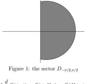
Figure 1: the sector D−π/2,π/2
i!d dtI
i
t(φ, ψ) = Iti(φ, Hψ) = Iti(Hφ, ψ). (30)
Proof: The first part of the theorem follows by a direct estimate. Equation (29) is a consequence of corollary 1, while equation 30 follows from Ito’s formula.
A stronger result, namely the equality
Iti(φ, ψ) = $φ, e−!iHtψ% (31)
cannot in general be proved in the case where H is given by (2). In fact, the analyticity argument used in the proof of corollary 1 cannot in general be applied to the proof of equality (31), as the following considerations show.
By theorem 5 the function f1 : ¯D−π/2,π/2 → C, defined by f1(z) =
$φ, e−z!Hψ%, is analytic on the sector D
−π/2,π/2 (shown in figure 1) and
continuous on ¯D−π/2,π/2 (as H has a positive spectrum and generates an analytic semigroup). On the other hand, as we have already seen, on the positive real line R+ the function f
1 can be expressed in terms
of a functional integral by means of the Feynman-Kac formula: $φ, e−z!Hψ% = zd/2 " Rd ¯ φ(√zx) " Ct e−zN +1λ! Rt 0| √ !ω(s)+x|2Nds ψ(√!√zω(t) +√zx)W (dω)dxdx (32) and the right hand side of (32) is well defined, if φ, ψ are sufficiently regular, when Re(zM +1) ≥ 0, i.e for z = |z|eiθ, with − π
2(M +1)+ k 2π M +1 ≤ θ ≤ π 2(M +1) + k 2π
M +1, k ∈ Z. i.e. on M + 1 different sectors of
the complex plane. In particular, the right hand side of (32) de-fines M + 1 different holomorphic functions gk with k = 0, . . . , M ,
−Π /6 Π /6 Π /2 5Π /6 7Π/6 3Π /2
Figure 2: The set of definition of the integral I(z)
each of them defined on a different sector of the complex plane, i.e. Dk := D− π 2(M +1)+k 2π M +1, π 2(M +1)+k 2π M +1, k = 0, . . . , M . As the M + 1 open
sectors are disjoint (actually the intersection of their closures contain a unique point), we cannot consider g0, . . . , gM as the same analytic
function defined on different regions of the complex plane. In particu-lar the analyticity properties of the left and the right hand side of (32) allows to extend the Feynman-Kac formula, if the condition of theorem 6 are satisfied, to all the values of z ∈ ¯D− π
2(M +1),2(M +1)π . This sector does
not include z = i (unless one considers the trivial case M = 0).
For instance, if 2M = 4 (the quartic oscillator case), the integral on the right hand side of (32) becomes
I(z) := zd/2 " Rd ¯ φ(√zx) " Ct e−z3λ! Rt 0| √ !ω(s)+x|2Nds ψ(√!√zω(t) +√zx)W (dω)dx. (33) Under analyticity and growing conditions on φ, ψ, the integral I(z) is well defined on three sectors ¯D−π
6,π6 ∪ ¯Dπ2,5π6 ∪ ¯D7π6 ,3π2 of the
com-plex z plane shown in figure 2. In particular the integral I(z) in (33) defines three analytic function g0, g1, g2 defined respectively on the
dis-joints domains D−π
6,π6, Dπ2,5π6 and D7π6 ,3π2 . They are analytic on their
domains of definition and continuous on the boundaries. However the information we have does not allow to prove that g0, g1, g2 are the same
analytic function, since the intersection of the closure of their definition domains is a single point, i.e. ¯D−π
6,π6 ∩ ¯Dπ2,5π6 ∩ ¯D7π6 ,3π2 = {0}.
holds for z belonging to ¯D−π 6,
π
6, but nothing can be said as it stands
for z = i. By these considerations, the Feynman path integral repre-sentation for the weak solution of the Schr¨odinger equation studied in [4] has to be interpreted in the weak sense of theorem 8.
The difficulties in the investigation on the relations between the func-tional integral (28) and the matrix elements of the Schr¨odinger group $φ, e−!iHtψ% can be better understood by means of the following
sim-plified model.
Let us consider the two functions of the complex variable λ, f1(λ) := " eiλx4+ix2dx f2(λ) := eiπ/4 " e−iλx4−x2dx
defined and analytic respectively on D1 = {Im(λ > 0)} and D2 =
{Im(λ < 0)}.
The function f1, for λ ∈ R λ < 0 can be seen as the one dimensional
analogue of $φ, e−!iHtψ%, while function f
2 as the one dimensional
ana-logue of the functional integral (28).
It is possible to verify by means of a rotation of the integration contour in the complex plane, that for λ ∈ R+ one has f
1(λ) = f2(λ).
For instance if λ = 1 one has ' eix4+ix2
dx = eiπ/4' e−ix4−x2
dx.
The extension of the equality between f1 and f2 on the negative real
line is, on the other hand, not possible. Indeed it is possible to see that f1 and f2 are different branches on an analytic multivalued function
defined on a Riemann sheet.
A transformation of variable allows us to represent the two functions in a fashion allowing us to enlighten their analyticity properties and the nature of the singularity in λ = 0. Indeed when λ ∈ R+, the following
equality holds f2(λ) = eiπ/4 " e−iλx4−x2dx = e iπ/4 λ1/4 " e−ix4−λ1/2x2 dx.
The right hand side is an analytic function in the region *λ ∈ C , λ = |λ|eiφ
: |λ| > 0, −π < φ < π+ .
It is continuous on the boundary of its analyticity domain but it is multivalued and it assumes different values approaching the negative real axis from above and from below:
f2(|λ|eiπ) =
"
f2(|λ|e−iπ) = eiπ/2
"
eiλx4−ix2dx
By a rotation technique it is easy to verify that the latter integral is equal to eiπ/2 " eiλx4−ix2 dx = eiπ/4 " e−iλx4−x2 dx.
In other words we can say that the two integrals ' eiλx4+ix2
dx and eiπ/4' e−iλx4−x2
dx do not coincide on the negative real line: they are different branches of the same analytic but multivalued function. In a similar way, the functional integral (28) and the matrix elements of the Schr¨odinger group can be interpreted, as functions of the complex variable λ, as different branches of the same analytic but multivalued function.
Remark 3. Despite the problems described so far, in the literature some particular cases have been handled by means of different tech-niques. In [22], equality (31) has been proved in the case where H is the inverse quartic oscillator Hamiltonian
H0ψ(x) = − !2 2∆ψ(x)+ 1 2xΩ 2 xψ(x)−λ|x|4ψ(x), ψ ∈ C02(Rd), λ ∈ R+, by means of an analytic continuation technique in the mass parameter.
In [13] the pointwise solution of the heat equation (19) and its func-tional integral representation have been considered:
(e−z!Htψ)(x) = " Ct e−zλ! Rt 0| √ !zω(s)+x|2Mds ψ0( √ !zω(t) + x)W (dω). (34) The right hand side of (34) evaluated for z = i gives
" Ct e−iλ! Rt 0| √ !iω(s)+x|2Mds ψ0( √ !iω(t) + x)W (dω). (35) For suitable exponents 2M , namely for Re(ei(M +1)π2) < 0, the integral
(35) is well defined and, as proved in [13] by means of a probabilistic argument, it represents the pointwise solution of Schr¨odinger equation. Let us consider now the integral (28) and let us assume that the hypothesis of theorem 8 are satisfied. By considering two suitable sets of vectors in S1, S2 ⊂ L2(Rd), with φ ∈ S2 and φ ∈ S1, it is possible
to interpret the integral Ii
t(φ, ψ) as the matrix element of an evolution
operator in L2(Rd).
Let us denote by S1 the subset of S(Rd) made of the functions φ : Rd→
C of the form
and by S2 the subset of S(Rd) made of the functions φ : Rd→ C of the
form
φ(x) = Q(x)e−x22 (1+i) (37)
where P and Q are polynomials with complex coefficients. As the Hermite functions form a complete orthonormal system in L2(Rd), it
is simple to verify that both S1 and S2 are dense in L2(Rd). Moreover
the functions φ ∈ S1 are such that:
(1) the function z *→ φ(zx), x ∈ Rd, z ∈ ¯D
0,π/4 is analytic on D0,π/4
and continuous on ¯D0,π/4,
(2) the function x *→ φ(eiπ
4x), x ∈ Rd is in L2,
while the functions φ ∈ S2 are such that:
(1) the function z *→ φ(zx), x ∈ Rd, z ∈ ¯D
−π/4,0 is analytic on
D−π/4,0 and continuous on ¯D−π/4,0,
(2) the function x *→ φ(e−iπ4x), x ∈ Rd belongs to L2(Rd).
Let us denote by T : S1 → S2 the linear operator defined by
T φ(x) = eiπ8dφ(eiπ4x), φ ∈ S1,
and by T−1 : S
2 → S1 its inverse, defined by
T−1φ(x) = e−iπ8dφ(e−i π
4x), φ ∈ S2.
By considering two vectors φ, ψ ∈ S1 one can easily verify that
$φ, T ψ% = $T φ, ψ%. (38)
Analogously, by considering two vectors φ, ψ ∈ S2, one can easily verify
that
$φ, T−1ψ% = $T−1φ, ψ%. (39) This implies that, for φ ∈ S2, ψ ∈ S1, one has $T−1φ, T ψ% = $φ, ψ%.
Let HT : S2 → S2 be the operator defined by −iHT := T HT−1. It
is easy to verify that HTφ(x) = −
!2
2 ∆φ(x) + λe
iM +12 π|x|2Mφ(x), φ ∈ S 2.
Theorem 9. Let ψ ∈ S1 and φ ∈ S2. Let us assume that Re(eiM +12 π) ≥
0. Then the operator HT is the restriction to S2 of the generator A of
a strongly continuous contraction semigroup V (t) = e−1!Atand the
inte-gral Ii
t(φ, ψ) given by (28) is equal to the matrix element $T−1φ, V (t)T ψ%.
Proof: Let V (t)t≥0 be the C0-contraction semigroup defined by the
Feynman-Kac type formula: V (t)ψ(x) := " Ct e−ei M +12 π λ!Rt 0| √! ω(s)+x|2Mds ψ(√!ω(t) + x)W (dω). (40)
The operator-theoretic results for semigroups of the form (40) have been investigated in [24, 20] (see also [18], chapter 13.5). In particular the generator A of the semigroup V (t) = e−t
!A is given on smooth vectors ψ ∈ S(Rd) by Aψ(x) = −! 2 2 ∆ψ(x) + Q2M(x)ψ(x), Q2M(x) := λe iM +1 2 π|x|2M (41) with domain D(A) = {ψ ∈ H1(Rd) : −! 2 2∆ψ + Q2Mψ ∈ L 2(Rd )}. (42) By a direct computation and by taking ψ ∈ S1 and φ ∈ S2, one can
easily verify that eiπ4d " Rd ¯ φ(eiπ4x) " Ct e−e i(M +1) π 2 λ ! Rt 0| √ !ω(s)+x|2Mds ψ(√!eiπ4ω(t) + eiπ4x)W (dω)dx = $T−1φ, V (t)T ψ% so that Ii t(φ, ψ) = $T−1φ, V (t)T ψ%.
Remark 4. Under the assumptions of theorem 9, it is possible to give an alternative proof of theorem 8, i.e. that the integral Ii
t(φ, ψ) is a
weak solution of the Schr¨odinger equation in the sense that equations (29) and (30) are satisfied.
Indeed equation (29) follows by writing Ii
0(φ, ψ) as $T−1φ, T ψ% and
by equations (38) and (39). Equation (30) follows from the equality Ii t(φ, ψ) := $T−1φ, e− t !AT ψ%. Indeed i!d dt$T −1φ, e−!tAT ψ% = $T−1φ, e− t !A(−iH T)T ψ% = $T−1φ, e− t !HTT Hψ%.
Remark 5. To prove that Ii
t(φ, ψ) = $φ, e− it
!Hψ% it would be sufficient
to have that |Ii
t(φ, ψ)| ≤ C+φ++ψ+, or, in other words, that given ψ ∈
S1, one has that the vector e− t
!HTT ψ belongs to the domain of (T−1)∗,
so that
$T−1φ, e−!tHTT ψ% = $φ, (T−1)∗e− t
!HTT ψ%.
If the inequality |Ii
t(φ, ψ)| ≤ C+φ++ψ+ holds true, then this would
namely imply that there exists a bounded operator B(t) : L2 → L2 such
that Ii
t(φ, ψ) = $φ, B(t)ψ% and B(0) = I. Iti(·, ·) defined on S2× S1 can
be extended to L2 × L2. In particular then Ii
t(U (t)φ, ψ) makes sense
and by differentiating with respect to the time variable t we obtain i!d
dtI
i
so that Ii
t(U (t)φ, ψ) = I0i(U (0)φ, ψ) = $φ, ψ% for any t and this implies
that B(t) = U (t).
5. The functional integral as asymptotic solution The present section is devoted to the proof that the functional inte-gral (28) coincides asymptotically both as t → 0 and as λ → 0 with the matrix element $φ, e!iHtψ% of the Schr¨odinger group.
Theorem 10. Let φ, ψ ∈ L2(Rd) and M ∈ N satisfy the assumptions of
theorem 9. Then as t → 0 the integral Ii
t(φ, ψ) and the matrix element
$φ, e!iHtψ% of the Schr¨odinger group admit the following asymptotic
ex-pansions Iti(φ, ψ) =%antn, $φ, e i !Htψ% = % bntn,
and they coincides, i.e. an= bn ∀n ∈ N.
Proof: By theorem 9, the functional integral Ii
t(φ, ψ) can be written
as $T−1φ, e−t
!AT ψ%, where A is the operator defined by (41) and (42).
Under the stated assumptions, the vector T ψ belongs to the domain of An ∀n ∈ N, and AnT ψ belongs to S
2 ⊂ D(T−1) ∀n ∈ N. In particular,
for any N ∈ N one has $T−1φ, e−!tAT ψ% = N % n=0 1 n! # − !t$n$T−1φ, AnT ψ% + R N, RN = 1 N − 1! # − !t$N " 1 0 uN −1$T−1φ, ANe−!tA(1−u)T ψ%du.
The remainder RN can easily be estimated by means of Schwarz
in-equality and one has: |RN| ≤ |t|
N|!|−N
N ! +T
−1φ++AN
T ψ+ = O(|t|N).
As T ψ ∈ S2, one has AnT ψ = (HT)nT ψ = inT Hnψ, so that by
equa-tion (39) $T−1φ, e−!tAT ψ% = N % n=0 1 n! # − it!$n$φ, Hnψ% + O(tN). Analogously $φ, e−it!Hψ% = N % n=0 1 n! # − it!$n$φ, Hnψ% + R$N,
R$N = 1 N − 1! # −it!$N " 1 0 uN −1$φ, HNe−it!H(1−u)ψ%du, with R$
N = O(tN), and one can easily verify that the asymptotic
ex-pansion in powers of t of Ii
t(φ, ψ) and of $φ, e− it
!Hψ% coincide.
Remark 6. The power series of the variable t are not convergent, but only asymptotic. This fact implies that the result theorem 10 is not sufficient to deduce the equality between Ii
t(φ, ψ) and $φ, e i !Htψ%.
Let us consider now couples of vectors φ, ψ satisfying the assumptions of theorem 1 (so that the result of theorem 4 holds) and such that the functional integral (28) is well defined. In fact, it is always possible to find a dense set of vectors in L2(Rd) satisfying both conditions. For
instance, if M = 2, it is sufficient to take ψ ∈ S1 and φ ∈ S2, while
if M ≥ 3 the fulfillment of hypothesis of theorem 1 implies that the integral (28) is well defined. Under these conditions, it is possible to interpret the functional integral (28) as an asymptotic weak solution of the Schr¨odinger equation, in the sense of the following theorem. Theorem 11. Under the assumptions above, the asymptotic expansion in powers of the coupling constant λ as λ → 0 of the functional integral representation (28) coincides with the corresponding asymptotic expan-sion (14) of the matrix elements of the Schr¨odinger group. Moreover the latter is Borel summable.
Proof: By expanding the functional integral (28) in powers of λ one has Iti(φ, ψ) = N −1 % n anλn+ RN, with an = 1 n!e iπ 4d " Rd ¯ φ(eiπ4x) " Ct # − e i(M +1)π2λ ! " t 0 | √ !ω(s) + x|2Mds$n ψ(√!eiπ4ω(t) + eiπ4x)W (dω)dx.
and RN = λN (N − 1)!e iπ 4d " 1 0 (1 − u) N −1" Rd ¯ φ(eiπ4x) " Ct # − e i(M +1)π 2λ ! " t 0 | √ !ω(s) + x|2Mds$Ne−ue i(M +1) π2 λ ! Rt 0| √ !ω(s)+x|2Mds ψ(√!eiπ4ω(t) + eiπ4x)W (dω)dxdu.
It is easy to verify that RN = O(λN). Moreover, by exploiting the
symmetry of the integrand, the coefficients an can be written as:
an = ei π 4d # − e i(M +1)π 2λ ! $n" t 0 . . . " t 0 ds1. . . dsn " Rd ¯ φ(eiπ4x) " Ct |√!ω(s1) + x|2Mds . . . |√!ω(sn) + x|2Mds ψ(√!eiπ4ω(t) + ei π 4x)W (dω)dx.
By the result of corollary 1, the latter coincides with the coefficient an
of the asymptotic expansion (14). On the other hand, by theorem 4, the matrix elements of the Schr¨odinger group can be obtained in terms of the Borel sum of the asymptotic expansion & anλn.
Remark 7. By a direct computation it is possible to verify that in the case M = 2 (the quartic oscillator case) the functional integral Ii
t(φ, ψ) can be extended to an analytic function of the variable λ in the
sector D0,π of the complex plane and satisfies there an estimate of the
following form |Iti(φ, ψ) − N −1 % n anλn| ≤ ACN|λ|NN !.
By Watson-Nevanlinna’s theorem, it is possible to recover Ii
t(φ, ψ) in
terms of the coefficients an in the asymptotic expansion. This result,
combined with the analogous result for $φ, e−i
!Htψ%, is not sufficient
to deduce the equality Ii
t(φ, ψ) = $φ, e− i
!Htψ%, as the two function are
defined as the Borel sums of the same asymptotic expansion but on different regions of the complex plane (the left hand side on D0,π and
the right hand side on Dπ,o). Indeed, let us consider two functions f1(z)
and f2(z) of the complex variable z, defined and holomorphic resp. in
estimate uniformly in their analyticity domains: f1(z) ∼ % anzn, |f1(z) − N −1 % n anzn| ≤ A1C1N|z|NN !, f2(z) ∼ % anzn, |f2(z) − N −1 % n anzn| ≤ A2C2N|z|NN !.
The function f1, f2can be recovered by their asymptotic expansion& anzn
by means of the following procedure. Let us define two functions g1(z)
and g2(z) of the complex variable z ∈ D−π/2,π/2 defined by
g1(z) := f1(iz), g2(z) := f2(−iz), z ∈ D−π/2,π/2.
g1 and g2 admit the following asymptotic expansion and estimate:
g1(z) ∼ % ina nzn, |g1(z) − N −1 % n ina nzn| ≤ A1C1N|z|NN !, g2(z) ∼ % (−i)nanzn, |g2(z) − N −1 % n (−i)nanzn| ≤ A2C2N|z|NN !.
By theorem 3 they are both Borel summable, i.e. formally: g1(z) = 1 z " ∞ 0 e−t/z%i na n n! t ndt, (43) g2(z) = 1 z " ∞ 0 e−t/z%(−i) na n n! t ndt. (44)
One would have f1(z) = f2(z) for z ∈ R+, if g1(iρ) = g2(−iρ) for
ρ ∈ R+, however the Borel summability of the asymptotic expansion
& anzn, in particular the relations (43) and (44), are by themselves
not sufficient to deduce this equality.
Acknowledgments
The hospitality of the Mathematics Institutes of Trento and of Bonn Universities is gratefully acknowledged, as well as the financial support of the F. Severi fellowship of I.N.d.A.M.
References
[1] S. Albeverio, R. Høegh-Krohn, S. Mazzucchi Mathematical theory of Feynman path integrals. An Introduction. 2nd and enlarged edition. Lecture Notes in Mathematics, Vol. 523. Springer-Verlag, Berlin-New York (2008).
[2] S. Albeverio, S. Mazzucchi, Generalized Fresnel Integrals, Bull. Sci. Math. 129, no. 1, 1–23 (2005).
[3] S. Albeverio, S. Mazzucchi, Generalized infinite-dimensional Fresnel Integrals, C. R. Acad. Sci. Paris 338 n.3, 255–259 (2004).
[4] S. Albeverio, S. Mazzucchi, Feynman path integrals for polynomially growing potentials, J. Funct. Anal. 221 no.1, 83–121 (2005).
[5] S. Albeverio, S. Mazzucchi, Some New Developments in the Theory of Path Integrals, with Applications to Quantum Theory, J. Stat. Phys. 115 n.112, 191–215 (2004).
[6] S. Albeverio, S. Mazzucchi, Feynman Path integrals for time-dependent poten-tials, in : “Stochastic Partial Differential Equations and Applications -VII”, G. Da Prato and L. Tubaro eds, Lecture Notes in Pure and Applied Mathematics, vol. 245, Taylor & Francis, (2005), pp 7-20.
[7] S. Albeverio, S. Mazzucchi, Feynman path integrals for the time dependent quartic oscillator. C. R. Acad. Sci. Paris 341, no. 10, 647–650. (2005).
[8] S. Albeverio, S. Mazzucchi, The time dependent quartic oscillator - a Feynman path integral approach. J. Funct. Anal. 238 , no. 2, 471–488 (2006).
[9] S. Albeverio, S. Mazzucchi, The trace formula for the heat semigroup with polynomial potential, SFB-611-Preprint no. 332, Bonn (2007).
[10] C. Bender, T. Wu, Anharmonic oscillator. Phys. Rev. (2) 184 (1969) 1231– 1260.
[11] I. M. Davies, A. Truman, On the Laplace asymptotic expansion of conditional Wiener integrals and the Bender-Wu formula for x2N-anharmonic oscillators.
J. Math. Phys. 24 , no. 2, 255–266 (1983).
[12] R.H. Cameron, A family of integrals serving to connect the Wiener and Feyn-man integrals, J. Math. and Phys. 39, 126–140 (1960).
[13] H. Doss, Sur une R´esolution Stochastique de l’Equation de Schr¨odinger `a Co-efficients Analytiques. Commun. Math. Phys., 73, 247-264 (1980).
[14] K.-J. Engel, R. Nagel, One-parameter semigroups for linear evolution equa-tions. With contributions by S. Brendle, M. Campiti, T. Hahn, G. Metafune, G. Nickel, D. Pallara, C. Perazzoli, A. Rhandi, S. Romanelli and R. Schnaubelt. Graduate Texts in Mathematics, 194. Springer-Verlag, New York, 2000. [15] Gross L., Abstract Wiener Spaces, Proc. 5th
Berkeley Symp. Math. Stat. Prob. 2, (1965) 31-42.
[16] G. H. Hardy, Divergent series, Oxford University Press, London (1963). [17] T. Hida, H.H. Kuo, J. Potthoff, L. Streit, White Noise Kluwer, Dordrecht
(1995).
[18] G.W. Johnson and M.L. Lapidus, The Feynman integral and Feynman’s oper-ational calculus. Oxford University Press, New York (2000).
[19] G. Kallianpur, D. Kannan, R.L. Karandikar Analytic and sequential Feynman integrals on abstract Wiener and Hilbert spaces, and a Cameron Martin For-mula, Ann. Inst. H. Poincar´e, Prob. Th. 21 (1985), 323-361.
[20] T. Kato, On some Schr¨odinger operators with a singular complex potential. Ann. Scuola Norm. Sup. Pisa Cl. Sci. (4) 5 , no. 1, 105–114 (1978).
[21] Kuo H.H., Gaussian Measures in Banach Spaces, Lecture Notes in Math., Springer-Verlag Berlin-Heidelberg-New York, (1975).
[22] S. Mazzucchi, Feynman path integrals for the inverse quartic oscillator, J. Math. Phys. 49, 9 (2008), 093502 (15 pages)
[23] S. Mazzucchi, Mathematical Feynman Path Integrals and Applications. World Scientific Publishing, Singapore (2009)
[24] E. Nelson, Feynman integrals and the Schr¨odinger equation, J. Math. Phys. 5 (1964), 332-343.
[25] F. Nevanlinna. Zur Theorie der asymptotischen Potenzreihen. Ann. Acad. Sci. Fenn. (A), 12 (3) (1919), 1-81.
[26] M. Reed, B. Simon, Methods of modern mathematical physics. II. Fourier anal-ysis, self-adjointness. Academic Press [Harcourt Brace Jovanovich, Publishers], New York-London, 1975.
[27] M. Reed, B. Simon, Methods of modern mathematical physics. IV. Analysis of operators. Academic Press [Harcourt Brace Jovanovich, Publishers], New York-London, 1978.
[28] B. Simon, Coupling Constant Analiticity for the Anharmonic Oscillator. An-nals of Physics 58, 76-136 (1970).
[29] B. Simon, Functional integration and quantum physics. Second edition. AMS Chelsea Publishing, Providence, RI, 2005.
[30] A. Sokal. An improvement of Watson’s theorem on Borel summability. J. Math. Phys. 21, 261-263, 1980.
[31] K. Yajima, Smoothness and Non-Smoothness of the Fundamental Solution of Time Dependent Schr¨odiger Equations, Commun. Math. Phys. 181, 605–629 (1996).
∗Institut f¨ur Angewandte Mathematik, Wegelerstr. 6, 53115 Bonn,
HCM; SFB611, BIBOS; IZKS; Dipartimento di Matematica, Universit`a di Trento, 38050 Povo, Italia
∗∗ Cerfim (Locarno), Acc. Arch.(USI) (Mendrisio). ∗∗∗ F. Severi fellow.