UNIVERSITY
OF TRENTO
DEPARTMENT OF INFORMATION ENGINEERING AND COMPUTER SCIENCE
38050 Povo – Trento (Italy), Via Sommarive 14
http://www.disi.unitn.it
IS PEER REVIEW ANY GOOD?
A QUANTITATIVE ANALYSIS OF PEER REVIEW
Fabio Casati, Maurizio Marchese, Azzurra Ragone, Matteo Turrini
August 2009
Technical Report # DISI-09-045
Preliminary Draft
Is peer review any good?
A quantitative analysis of peer review
Preliminary Draft
Fabio Casati, Maurizio Marchese, Azzurra Ragone, Matteo Turrini
Universita degli studi di Trento, Trento, Italy
{casati,marchese,ragone,turrini}@disi.unitn.it
Abstract. In this paper we focus on the analysis of peer reviews and reviewers behavior in conference review processes. We report on the development, defini-tion and radefini-tionale of a theoretical model for peer review processes to support the identification of appropriate metrics to assess the processes main properties. We then apply the proposed model and analysis framework to data sets about reviews of conference papers. We discuss in details results, implications and their even-tual use toward improving the analyzed peer review processes. Conclusions and plans for future work close the paper.
1 Introduction
Review systems are primarily used both for assessing the quality of a given work and, consequently, to provide hints about the reputation of the author who crafted it. The role of this activity is fundamental, in order to increase the quality and productivity related to a particular scientific area and also in credits assignment.
In this sense, the goal of our work is to understand the characteristics of the review systems available nowadays in academia. In parallel, there is the need of highlighting weaknesses and strengths of the process and of studying aspects potentially related to two core features that should, in principle, characterize every evaluation system: fairness and efficiency. Once all those aspects have been sufficiently understood, there might be the possibility to propose new models for the evaluation, that could provide further metrics and algorithms for setting up the process more easily, also trying to get some improvements.
We start from the definition of a theoretical model for peer reviews to support the identification of appropriate metrics to assess relevant properties of the review pro-cesses, that could help, then, to improve the process itself. Specically, we aim at a peer review process that allows the selection of high quality papers and proposals, that is fair and efficient (in terms of minimizing the time spent by both authors and reviewers).
The outcome of this line of work has been the definition of metrics:
– to identify and understand correlation between different ranking criteria and assess-ment phases;
– to analyzes the robustness of the evaluation process to stochastic perturbation of the marks distribution; this allow us to quantify and put in the proper scale the computed values of disagreement and rating biases
– to identify and understand the average level of disagreement and rating biases present in the process and the assessment of compensation methods
– to compute efficiency related metrics, such as correlation and minimal number of reviews.
All these information are useful to better characterize the different evaluation processes, making these more open and transparent and indicating ways to improve them. Once the model and the analysis tools have been defined, we have applied them to data about re-views of conference papers. Interesting aspects of the review system have been inferred from the analysis, which could help in the understanding of such complex process. In brief, for the specific analyzed data sets:
– there is a significant degree of randomness in the review process, more marked than we initially expected; the disagreement among reviewers sometimes is pretty high and there is very little correlation between the rankings of the review process and the impact of the papers as measured by citations. Furthermore, in the majority of the studied cases rankings and acceptances are sensitive to variations in the marks given by reviewers;
– it is always possible to identify groups of reviewers that consistently give higher (or lower) marks than the others independently from the quality of the specific proposal they have to assess. Moreover, we show that our proposed unbiasing procedure can have a significant effect on the final result. This information and proposed unbias-ing tool could be useful to the review chairs to improve the fairness of the review process
– Here we show that it is possible to minimize efforts without compromising quality by reducing the number of reviews on papers whose fate is clear after, for instance, only a couple of reviews.
2 Modeling and measuring peer reviews
This section describes a model for peer reviews and identifies metrics that help us assess properties of the reviews. We focus specifically on:
– modeling peer reviews of scientific papers.
– identifying metrics that help us understand and improve peer reviews. Specifically, we aim at a peer review process that allows (i) the selection of high quality papers and proposals , that is fair, and that is efficient (in terms of minimizing the time spent by both authors and reviewers).
In the subsequent sub-sections we will present and discuss appropriate definitions for what we mean by quality, fairness and efficiency. The model and metrics provided in this section are generally applicable to a variety of review processes, and can be used as a benchmark framework to evaluate peer reviews, also beyond the experimental results provided in this document.
2.1 Peer review model
This section formally defines and abstracts the peer review process. The level of ab-straction and the aspects of peer reviews that are abstracted are driven by the goal of the work and the metrics we want to measure, discussed in the next section.
From a process perspective, peer reviews may vary from case to case, but usually they proceed along the following steps. Authors submit a set C = {C1, . . . , Cn} of
contributions1for evaluation by a group E of experts (the peers, also called reviewers).
Contributions are submitted during a certain time window, whose deadline is ds. Each
contribution is assigned to a number of reviewers and its flow through the process can be supervised by senior reviewers (a set SR ⊂ E of distinguished experts that analyze reviews and help chairs take a final decision on the contribution). The assignment can be
continuous (contributions are assigned as they come, as in the case of journals or some
projects proposal) or in batch, and can be done in various ways (e.g., via bidding, based on topics, or based on decisions by chairs). In most processes, the number of reviewers
NRinitially assigned to review or supervise each contribution is predefined and equal
for all contributions. The typical settings for conferences is to have three reviewers and zero or one senior reviewer per paper. In the general case, each contribution may be assigned to a different number of reviewers.
The review occurs in one or more phases. We denote with NP the total number of
phases. In each phase pk, contributions are assigned, marks are given, and contributions
that are allowed to proceed to the next phase are selected. The next phase may or may not require authors to send a revised or incremental version of the contribution. At the end of each phase there is a discussion over the reviews (possibly involving author feedback). Some processes require the discussion to end in a “consensus” result for each of the marks. In all cases, the discussion results in a decision on whether each contribution is accepted or not. The entire process is supervised by a set CH ⊂ E of
chairs.
For example, the typical conference has a one-phase review, with discussion at the end leading to acceptance or rejection of each paper. Some conferences, such as Sigmod, have a 2-phase review process where in the first phase each paper is assigned to two reviewers and only papers that have at least one accept mark go to phase 2 and are then assigned to a third reviewer. This is done to minimize the time spent in reviewing. EU FET-Open proposals also follow a 2-phase process, where proposals are assigned to three reviewers in each phase and where authors send a revised and extended version of the proposal in phase 2. This is done to minimize both the reviewing effort and the proposal preparation effort (only a few groups can submit long proposals).
Given the above, we model a phase pkof a peer review process as follows:
Definition 1. A phase p = (C, E, M, π, γ, σ, ρ, A) of a peer review process consists of:
– a set C = {C1, . . . , Cn} of contributions submitted for evaluation;
– a set E of experts, which includes:
• a set CH ⊂ E of chairs that supervise the review process
1Notice that in the rest of the paper we use both the terms contribution and paper with the same meaning
• a set SR ⊂ E of distinguished experts (sometimes called senior reviewers) that analyze reviews and help chairs take a final decision on the contribution
• a set R ⊆ E of experts that act as reviewers of the contributions and s.t. CH ∪ SR ∪ R = E
– a set M of mark sets, ={M1, . . . , Mq}, where for each mark set a total order
relation ≤ always exists. For each mark set Mjthere is a distinguished value called
acceptance threshold, denoted by tj.
– an assignment function π : C −→ P(R) × P(SR) assigning each contribution to a subset of the reviewers and a subset of the senior reviewers (an element of the respective powersets).
– a scoring function γ : {c, r} −→ M1× . . . × Mq such that c ∈ C and r ∈ π(c).
This function models the marks assigned by each reviewer.
– a score aggregation function σ : M1× . . . × Mq −→ N. This models the way in
which in some review processes one can derive an aggregate final mark based on the individual marks.
– a ranking function ρ : {c} −→ N
– a subset A ⊂ C that denotes the accepted contributions.
In the rest of the section we will refer to a simple example in order to explain the metrics used in the peer review evaluation process.
EXAMPLE 1. Consider a review process with: – |C| = 10 submitted contributions;
– |E| = |R| = 5 experts that act as reviewers and no chairs (|CH| = 0) or senior
reviewers (|SR| = 0);
– a set of three criteria: M1 = quality, M2 = implementation, M3 = impact,
where for each criteria Mjthe reviewer can assign a mark whose domain is the set
of integer {1, . . . , 10};
– the number of contributions assigned to each reviewer NRC = 3.
We next define metrics for peer review that are then computed over the review data in our possession. The purpose of such metrics is to help us understand and improve peer reviews under two dimensions: quality and efficiency. Informally, quality is re-lated to the final result: a review process ensures quality if the best contributions are chosen. Efficiency is related to the time spent in preparing and assessing the contribu-tions: a process is efficient if the best proposals are chosen with minimal time spent both by authors in preparing the contribution and by reviewers in performing the reviews. This is consistent with the main goals of peer reviews: selecting the best proposals with the least possible effort by the community. As we will see, both quality and efficiency are very difficult to measure. Notice that in this document we disregard other potential benefits of peer reviews, such as the actual content of the feedback and the value it holds for authors. We focus on metrics and therefore on what can be measured by looking at review data.
2.2 Quality-related metrics
In an ideal scenario, we would have an objective way to measure the quality of each contribution, to rank contributions or to, at least, select ”acceptable” contributions from others. If this was the case, we could measure the quality of each peer review process execution, and identify which processes are more likely to be of high quality. Unfortu-nately (or fortuUnfortu-nately, depending on how you see it) it turns out that quality is subjective, and there are no objective or widely accepted ways to measure quality. Nevertheless, we think it is possible to define metrics that are approximate indicators of quality (or lack thereof) in a review process and use them in place of the ideal ”quality”. An im-portant subclass of these metrics are those related to fairness, which study whether the authors got a fair chance for their contribution to be accepted. In the next sub sections we explore the rationale behind a number of proposed quality-related metrics. We then detail their definitions and present some simple examples to illustrate their potential application.
Divergence from the ideal ranking In this metric we do assume that, somehow, we have the “correct” or “ideal” ranking for the contributions. We can assume or imagine that this can be conceptually measured in some way. For example, the ideal ranking could be the one each of us defines (in this case the comparison is subjective and so is the value for the metric), or we can define it as the ranking that we would have obtained if all experts reviewed all contributions (as opposed to only two or three reviewers).
In such a case we could try to assess how much the set of the actual accepted contri-butions differs from the set of the contricontri-butions that should have been accepted accord-ing to the ideal rankaccord-ing. More formally, we can define a measure called divergence, in order to compute the distance between the two rankings, i.e., the ideal ranking and the
actual ranking (the outcome of the review process). We next give the formal definition
of divergence following Krapivin et al. [2], adapted to our scenario.
Definition 2 (phase quality divergence). Let C be a set of submitted contributions,
n = |C| the number of submissions, ρi and ρa, respectively, the ideal ranking and the
actual ranking, and t the number of accepted contributions according to the actual ranking. We call divergence of the two rankings Divρi,ρa(t, n, C) the number of
ele-ments ranked in the top t by ρithat are not among the top t in ρa.
The normalized divergence N Divρi,ρa(t, n, C) is equal to
Divρi,ρa(t,n,C)
t , and varies
between 0 and 1.
Therefore, through this metric it is possible to assess how much the set of the ac-tual accepted contributions diverges from the set of contributions ranked w.r.t. the ideal quality measure, and so how many contributions are ”rightly” in the set of the accepted
contributions and how many contributions are not.
One can also compute the divergence for each reviewer, considering, instead of the whole set of contributions, only those contributions rated by a particular reviewer, i n order to assess, instead of the quality of the entire process, the quality of a specific reviewer.
Definition 3 (reviewer quality divergence). The reviewer quality divergence Divρi,ρa(tr, nr, Cr)
is defined analogously to the phase quality divergence with the difference that we re-strict the divergence computation to the set Crof contributions reviewed by reviewer r
instead of the entire set of submissions C (so, nr= |Cr| is the number of contributions
reviewed by r, accepted and rejected ones, and ranked, and tris the number of
con-tributions reviewed by r whose score is equal or greater than the contribution in the accepted set with the lowest score), as per the scoring function.
The normalized reviewer quality divergence N Divρi,ρa(tr, nr, Cr) is given by
N Divρi,ρa(tr, nr, Cr) =
Divρi,ρa(tr,nr,Cr)
tr .
Divergence a posteriori One may argue that quality can be measured a posteriori (years after the completion of the review process), by measuring the impact that the paper had, for example by counting citations. Hence, we can compare this ranking a posteriori with the one coming out of the review process. However, we can do this only for accepted papers, since for rejected ones we do not have a way to assess their impact (they have not been published, or at least not in the same version as they were submitted).
As done before, we could use the divergence measure, using as metrics the
citation-based estimates and the actual ranking of contributions, but restricting the analysis to
the set of accepted contributions A instead of C, as only for those we have the two rankings. In this case, in the divergence formula, t would be equal to n and divergence would be always zero. We can still use divergence as an analysis mean, but only if we restrict to, say, examining the difference in the ranking in the top k contributions, with
k < t.
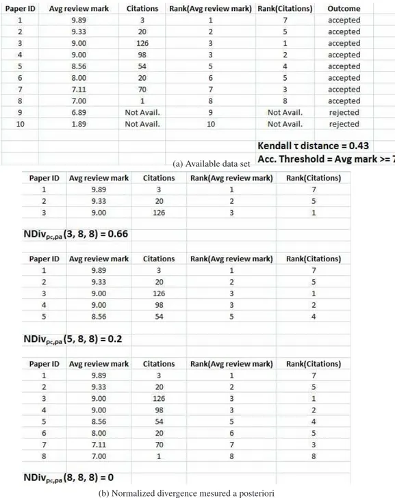
For instance, following Example 1, in Figure1we can compute the divergence with respect to the top contributions. In Fig.1awe show the example data set. Contributions are ranked with respect to the actual ranking (the one resulting from the review process). For each contribution we show: (i) the overall score given by the reviewers, computed as the average over all the three criteria, (ii) the number of citations that the contribution received (say after 3 years from publication), (iii) the actual ranking, (iv) the citation-based ranking, (v) the outcome (accepted/rejected) for each paper.
In Fig.1bwe compute how many elements in the top t are different between the two rankings. For instance, we compute for t = 3: N Divρc,ρa(3, 8, 8) = 0.66, with ρc =
Citation-based ranking, ρa= Actual ranking, and for t = 5: N Divρc,ρa(5, 8, 8) = 0.2.
Please note that by definition of the divergenge metric, we have N Divρc,ρa(8, 8, 8) =
0.0. We want to underline that the result for t = 3 indicates a high divergence between the two rankings. It means that 66% of the times the two rankings are different and this would lead to a 66% difference in the probability of acceptance of a contribution if we would accept 3 out of 8 contributions, which corresponds to ca. 37% acceptance ratio, i.e., a typical acceptance ratio. This mean that we are doing wrong choices while select-ing contributions in the 66% of the cases, which is a huge value. Probably, extendselect-ing this analysis to a greater number of contributions (say, 30 out of 80), the divergence value will be lower, still, one should compute which is an acceptable, or, say, ideal di-vergence value that could be accepted for a peer review process, in order to consider the review process a quality review process, that is a process that gives different results
w.r.t. a simple random selection of the contributions. This is the focus of our current investigation; moreover, once such a value has been computed, one can try to estimate the effort required w.r.t. this ideal divergence value (see Section2.3).
Another useful metric we can use in our evaluations is the Kendall τ distance, the typical metric for measuring a difference between two rankings [1]. The Kendall τ distance - differently from the divergence which computes only the number of elements that differs between two sets - computes the difference in the position of the elements between two sets. Therefore is more useful than the divergence measure when the two sets to compare have the same number of elements, as when the two sets to compare are
only the accepted contributions ranked using the actual ranking and the citation-based
ranking.
Definition 4 ( Kendall τ distance). Let ρ1and ρ2be two different rankings, the Kendall
τ distance is measured as the number of steps needed to sort bi-ranked items so that any pair A and B in the two rankings will satisfy the condition:
sign(ρ1(A) − ρ1(B)) = sign(ρ2(A) − ρ2(B))
In our setting, given the actual ranking ρaand the citation-based ranking ρcwe can
compute the Kendall τ distance for any pair of contributions ciand cjin the set of the
accepted contributions A, satisfying the condition:
sign(ρa(ci) − ρa(cj)) = sign(ρc(ci) − ρc(cj))
As before, while the above definition is given for the whole process, an analogous metric can be defined to analyze each single reviewer (as long as a reviewer had to rank/rate contributions that have been accepted and therefore have an associated citation count). In this case the Kendall τ distance is computed for any pair of contributions ci
and cjin the set of the accepted contributions reviewed by r.
The Kendall τ distance is typically normalized (N Kτ) by dividing it by n(n−1)2
(which is the maximum value, corresponding to lists ordered in the opposite way), so that the distance is in the [0,1] interval.
Referring to Example 1, we can compute the normalized Kendall τ distance N Kτ
for the set of contributions (see Fig.1a), taking into account the two rankings: the actual ranking (Rank(Avg review mark)) and the citation-based ranking (Rank(Citations)). In particular, we have that:
N Kτ= 0.43
The values of the normalized Kendall τ distance are always in 0 ≤ N Kτ ≤ 1.
If N Kτ = 1 this means that the ranked items are always in a different position with
respect to the two rankings, while if N Kτ = 0 the two rankings produce the same
ordered list. In this case the normalized distance is N Kτ = 0.43, meaning that the
review process in the example has performed rather poorly with respect to the selected
(a) Available data set
(b) Normalized divergence mesured a posteriori
Fig. 1: Normalized divergence: sample of 8 accepted contributions (n = 8), with respect to the top ranked (t = 3 and t = 5)
An ongoing analysis we are performing is on to try to estimate the Kendall τ trend, that is try to predict the value of Kτ for all contributions (accepted and not accepted
ones), based on the value and distribution of the Kτfor the set of accepted contributions.
Another useful metric is the Kendall τ rank correlation coefficient [1] that measures the degree of correspondence between two rankings, so assessing the significance of this correspondence.
Definition 5 (Kendall τ rank correlation coefficient). Let nc be the number of
con-cordant pairs and nd the number of discordant pairs in the data set, and n the total
number of contributions, we define the Kendall τ rank correlation coefficient as follow: τ = 1nc− nd
2n(n − 1)
The coefficient τ can assume the following values: – τ = 1, the two rankings are the same;
– τ = −1, one ranking is exactly the reverse of the other;
– τ = 0, the two rankings are completely indipendent.
Obviously, for values such that 0 ≤ τ ≤ 1, increasing values of τ imply increasing agreement between the two rankings, while for −1 ≤ τ ≤ 0 decreasing values of τ imply increasing disagreement between the two rankings.
Disagreement between referees Through this metric we compute the similarity be-tween the marks given by the reviewers on the same contribution. In particular, given a specific criterion j, we compute how much the marks of a reviewer i differ from the marks of the other r − 1 reviewers (Definition6), Then we compute for a specific crite-rion j the disagreement of a reviewer i with respect to the others over the whole set of contributions (Definition7), and, finally, over all the criteria (Definition8).
The rationale behind this metric is that in a review process we expect a high agree-ment between reviewers. It is natural that reviewers have different opinions on contri-butions. However, if the marks given by reviewers are comparable to marks given at random and have high disagreement, then the results of the review process are also ran-dom, which defeats the purpose. The reasons for having reviewers (and specifically for having 3 reviewers, the typical number) is to evaluate based on consensus or majority opinion.
Intuitively, assume that we consider the ideal ranking to be the one that we would obtain by having all experts review all papers, and that we assigned each contribution to only 3 reviewers to make the review load manageable. If the disagreement is high on most or all contributions, we cannot hope that the opinion of 3 reviewers will be a reasonable approximation or estimate for the ideal ranking. We will get back to this issue when discussing the quality vs effort trade-off.
In order to measure the disagreement, we compute the euclidean distance between the marks given by different reviewers on the same contribution.
Definition 6 (Disagreement of a reviewer on a criterion). Let j be a criterion and
z. Then, a disagreement φjiz among rzreviewers on a contribution z is the euclidean
distance between the mark given by the reviewer i, and the average µjiz of those given by the others r − 1 reviewers:
φjiz=| Mjiz-µjiz| (1) with: µjiz= 1 rz · rz X k6=iz Mjkz (2)
Definition 7 (Disagreement of a review phase on a criterion). Let n be the number of
the contributions and rzbe the number of reviewers assigned to a contribution z, then
the disagreement over all contributions on a criterion j is the average disagreement:
Φj= 1 n· n X z=1 ·1 rz rz X k=1 φjk z (3)
Definition 8 (Disagreement of a review phase). Let q be the number of criteria in a
review phase, then the disagreement over all the criteria is:
Ψ = 1 q· q X j=1 Φj (4)
Analogously to the above definitions and via obvious extensions we can also define: Definition 9 (Disagreement of a reviewer on a contribution). Let q be the number of
criteria in a review phase, then the disagreement of a reviewer i on a contribution z is: γiz= 1 q· q X j=1 φjiz (5)
Definition 10 (Average disagreement of a reviewer). Let Z be the number of
contri-butions a reviewed by a reviewer i, then the average disagreement of a reviewer i is: γi = 1 Z· Z X z=1 γiz (6)
Definition 11 (Disagreement of a review phase on a contribution). Let rz be the
number of reviewers in a review phase on a contribution z, then the disagreement of a review phase on a contribution is:
Γz = 1 rz · rz X i=1 γiz (7)
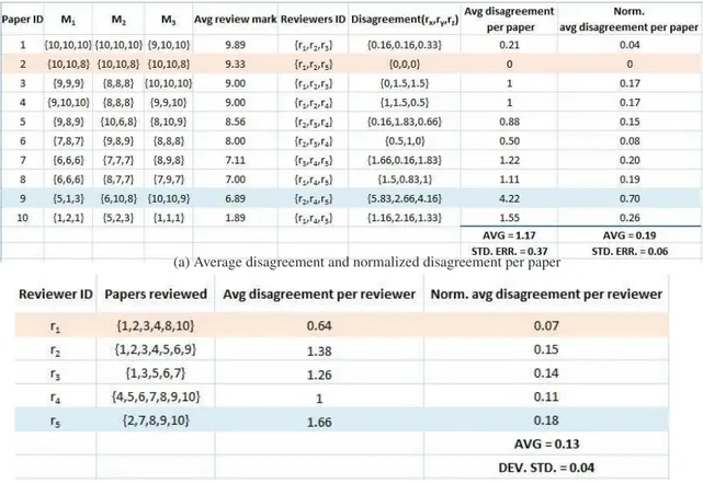
To illustrate operatively the disagreement metric, we use again the data from Exam-ple 1 in Figure2and compute the disagreement for each paper and each reviewer, w.r.t. the the others two reviewers. For each paper (Paper ID) we have (i) the marks given by
each reviewer for a given criterion (M1, M2, M3), (ii) the average score obtained by
each contribution after the review phase (Avg review mark)), (iii) the reviewers that have had that contribution in charge, (iv) the disagreement value computed for each reviewer and over all the criteria, (v) the average disagreement per paper and (vi) the normalized average disagreement for paper.
The minimum average disagreement among reviewers is zero, while - in this specific set - the maximum potential average disagreement is 6, corresponding to the following mark assignment: M1(1,1,1), M2(10,10,10), M3(10,10,10). Notice that for paper ID=2
the disagreement is zero, while the highest disagreement pertains to paper ID=9. More-over, we can compute the average disagreement of the overall (specific) review process, as well as its variance (absolute and normalized values are included in Figure2).
(a) Average disagreement and normalized disagreement per paper
(b) Average disagreement and normalized disagreement per reviewer
Fig. 2: (Normalized) disagreement calculated on the data set
If the disagreement value, given three reviewers for each contribution, is high this means that, probably, three reviewers are not enough to ensure a high quality review process. Indeed, having a high disagreement value means, in some way, that the
judg-ment of the three peers is not sufficient to state the value of the contribution itself. So this metric could be useful to improve the quality of the review process as could help to decide, based on the disagreement value, if three reviewers are enough to judge a con-tribution or if more reviewers are needed in order to ensure the quality of the process. Robustness A mark variation sensitivity analysis is useful in order to assess if a slight modification on the value of marks could bring a change in the final decision about the acceptance or rejection of a contribution.
The rationale behind this metric is that we expect the review process to be robust to minor variations in one of the marks. In a way we can see it as yet another measure of randomness in the review process. When reviewers need to select between, say, a 1-10 score for a set of metrics, often they are in doubt and perhaps somewhat carelessly decide between a 7 or an 8 (not to mention the problem of different reviewers hav-ing different scorhav-ing standards, discussed next). With this metric we try to assess how much precision is important in the mark assignment process, i.e., how much a slight difference in the mark value can affect the final (positive or negative) assessment of a contribution. To this end, we apply a small positive/negative variation ² to each marks (e.g., ±0.5), and then rank the contributions with respect to these new marks. Assuming that we accept the top t contributions, we then compute the divergence among the two rankings in order to discover how much the set of accepted contributions differs after applying such a variation.
Definition 12 (naive ²-divergence). Let ρabe the actual ranking and ρsbe the ranking
after the mark variation phase, C a set of contributions, n = |C| the number of contribu-tions submitted and ranked according to ρaand ρs, and t = |CA| the number of actually
accepted contributions, we call divergence of the two rankings Divρa,ρs(t, n, C) the
number of elements that differ between the two sets (or, t minus the number of elements that are equal)
The higher the divergence, the lower the robustness. Intuitively, what we do with the mark variation is a a naive way to transform a mark into a random variable with a certain variance, reflecting the indecision of a reviewer on a mark. Reviewers do have indecision among similar marks especially if the number of possible marks for a criterion is high. Informally, if we assume that each reviewer has an indecision area for the mark (e.g., in case of a 1-10 scoring range, we assume that a reviewer has a hard time discriminating between, say, a 6 and a 7), when the process is not robust to some marks differing of 1 from the actual ones, then it means that a more or less random decision between a 6 and a 7 given by a reviewer can determine the fate of the contribution. Notice that a process that is not robust is not necessarily low quality. For example, if for a criterion we have only two marks, 0 and 1, it is natural that the process is not robust but the granularity of the mark set is so coarse that it is unlikely for the reviewer to be undecided. The problems arise when the granularity is fine and the robustness is low.
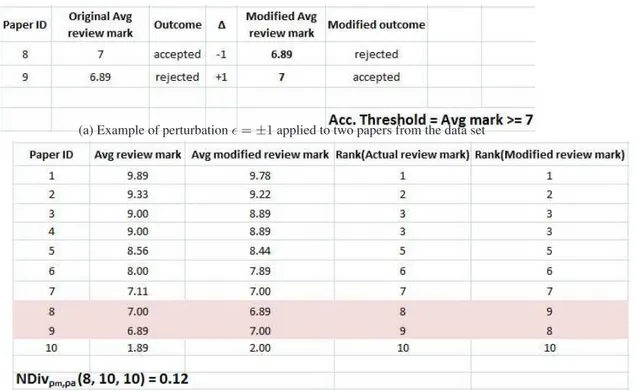
To illustrate operatively the mark sensitivity analysis, we use again the data from Example 1. In Fig.3awe modify the marks given to one of the contributions taken from the data set of Example 1, by subtracting ² = 1 in turn to each of the three marks given
(a) Example of perturbation ² = ±1 applied to two papers from the data set
(b) Normalized divergence calculated between the rankings obtained before and after the perturbation ², where ² =
−1 for accepted papers and ² = +1 for rejected papers
by the three reviewers. Then, we fix an acceptance threshold and see how the acceptance changes according to the small modification we made to the marks assigned. In our simple case, changing the average review mark given to paper with ID=8 and paper with ID=9 also changes the acceptance of them. In fact, in this case we applied ² = −1 to paper with ID=8 and ² = +1 to paper with ID=9 and we see that the recomputed average essentially swaps them in the ranking. So, in the perturbated case we have that paper with ID=8, which was accepted, is now rejected and, conversely, paper with ID=9, which was rejected, is now accepted.
This computation can be extended to all papers and the results for our data from Example 1 (see Fig.3b). We applied such modification to the entire data set of papers, subtracting ² = −1 to the accepted papers and adding ² = +1 to the two papers that were rejected. After we computed the new ranking obtained from the perturbation ², we calculate the normalized divergence N Divρm,ρa(8, 10, 10) between the rankings
obtained with and without the ² modification. The normalized divergence we found actually tells us that the ranking has been slightly modified and in particular that the set of accepted papers is changed.
The statistical version of the above metric is the ²-robustness. With this metric, we replace each mark m with a random variable M uniformly distributed between m − ² and m + ² (this distribution represent the reviewer’s uncertainty). When we do this, rankings become stochastic, so each ranking ρ has a certain probability of occurring. We call this stochastic ranking deriving from the perturbation of the marking as ρ².
Definition 13 (²-divergence). Let ρa be the actual ranking and ρ² the random
vari-able defining rankings after perturbations. Let C be a set of contributions, n = |C| the number of contributions submitted, and t = |CA| the number of actually accepted
contributions. We call stochastic divergence of the two rankings Divρa,ρ²(t, n, C) the
random variable denoting the probability that the divergence between ρaand the
(ran-dom) ranking ρ²has a given value ².
Definition 14 (δπ-robustness). We say that a ranking is ²-robust if the probability of
the ²-divergence being less than δ is equal or greater than π.
In this way we can compute the robustness of the process and see how much the process is sensitive to the mark variation.
Fairness-related metrics A property that, we argue, characterizes a “good” review process, and specifically the assignment of contributions to reviewers, is fairness.
A review process is fair if and only if the acceptance of a contribution does not depend on the particular set of reviewers that assesses it among the set of experts E. Formally, assume that we are able to compute, at the start of the review process (af-ter the contributions have been submitted but before they are assigned) the probability of a contribution c being accepted. We denote this probability as Pc
accept(tstart).
As-sume now that we can compute the same probability after the contributions have been assigned to reviewers. We denote this probability as Pc
accept(tassign).
We define an assignment process as fair with respect to contribution c iff:
In other words, an assignment is unfair if the reviewers selected for contribution c give marks which are different than what a randomly selected set of reviewers (among the committee members) would give.
Correspondingly, we define a peer review process as fair iff:
Pc
accept(tstart) = Pacceptc (tend) ∀C ∈ C
where Pc
accept(tend) is the probability of the final acceptance of the contribution2.
The problem with unfair assignments is that the assignment is affecting or determin-ing the fate of the paper: a different assignment would have yielded a different result. Again, to a certain extent, this is normal, natural, and accepted: different reviewers do have different opinions. The problem we are trying to uncover is when reviewers are
biased in various ways with respect to their peers. For example, a common situation is
the one in which a reviewer is consistently giving lower marks with respect to the other reviewers for the same contributions, perhaps because he or she demands higher quality standards from the submission.
Our aim is not to try to identify what is the appropriate quality standard or to state that reviewers should or should not be tough. However, if different reviewers have dif-ferent quality standards, when a contribution has the “bad luck” of being assigned to one such tough reviewer, the chances of acceptance are lower. This has nothing to do with the relative quality of the paper with respect to the other submissions, it is merely a biasing introduced by the assignment process and by the nature of the reviewer, that is rating contributions using, de facto, a different scale than the other reviewers. Fairness metrics try to identify, measure, and expose the most significant biases so that the chair can decide if they indeed correspond to unfair review results that need to be compen-sated before taking the final decision. As such they can be indicators of quality but also can provide hints to the chairs to compensate quality problems. In the following we illustrate different kind of biases and define a metric to discover biased reviewers.
– Rating bias: Reviewers are positively biased if they consistently give higher marks than their colleagues who are reviewing the same proposal. The same definition applies for the opposite case, when we talk about negatively biased reviewers. We also refer to these two cases as accepting behavior and rejecting behavior. – Affiliation bias: it is a rating bias but computed over contributions written by
au-thors with certain affiliations.
– Topic bias: a rating bias but computed over contributions concerning certain topics or research areas.
– Country bias: a rating bias but computed over contributions whose authors are coming from a certain country or continent (for instance, American reviewers with respect to papers written by European authors).
– Gender bias: a rating bias but computed over contributions written by authors of a certain gender.
2Between t
assign and tend the probability could change because the contribution has been
revised, a senior reviewer entered the process, an author feedback is provided, or a de-bias phase is performed.
– Clique bias: a rating bias but computed over contributions written by authors which belong to the same clique inside a certain research community.
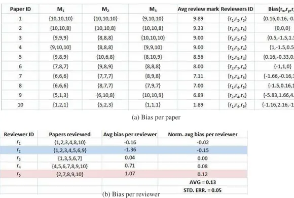
The way to compute the bias value is very similar to that described for the disagree-ment metric (see Definition 6), the difference is that the domain may be restricted to papers with certain topics or affiliations (depending on the kind of bias we are looking at), and that the sign of the disagreement coefficient φji has been preserved, basically replacing equation (1) with the following one:
φji = Mji-µji (8) This time the sign of the equation is important in order to discover positive or negative biases. Indeed, if the value of φji is constantly positive, this means the reviewer tends to give always higher marks with respect to other reviewers; while if the value of φji is constantly negative then the reviewer tends to give always more negative marks than other reviewers.
A variation on the rating bias is the variance bias, which occurs when a reviewer always gives marks that are very close to (or far from) the threshold for a mark. This is computed by simply calculating the variance of the mark.
As for the disagreement metrics, there are several scopes to which we can apply the bias metric. For example, we can measure the bias for a single reviewer and for a particular criterion, the bias over a review phase, and the bias over all the criteria. In the experiments we will assess the biases on actual review data and discuss how they can be compensated.
In Fig.4we first report the computed bias per reviewer per paper for the data of Example 1 and then the computed average bias per reviewer in which we highlighted the most accepting behavior and the most rejecting behavior. This information could be useful to a Conference Chair to improve the fairness of the review process.
We now address the difference between the actual ranking and the ranking obtained by compensating the biases. To compensate, we modify the marks by adding or remov-ing the bias values so that on average the overall bias of the most biased reviewers is reduced. In particular, we take all reviewers r that have a bias greater than b and that have done a number of reviews higher than nr, and subtract b from all marks of r (or from the top-k biased reviewers). We call this ranking debiased ranking ρb,nr.
Definition 15 (bias compensation divergence). It is the value Divρa,ρb,nr(t, n, C)
2.3 Efficiency-related metrics
Efficiency refers to the effort spent in determining which contributions are accepted, and in particular the trade-off between effort and quality of the review process. It considers both the effort in writing contributions and in reviewing them.
Assumptions The basic working assumption of this section is that the quality-effort trade-off exists and that, in general, if a paper or proposal is long, and is reviewed very
(a) Bias per paper
(b) Bias per reviewer
the selection is more informed than the case in which, say, one page proposal is briefly looked at by a couple of reviewers. Time is a precious resource, so the challenge is how to reduce the time spent while maintaining a “good” selection process that indeed selects the “best” proposals. A separate issue that we do not address (also as it is hard to measure) is the fact that a process is affected by the quality of the reviewers and the amount of discussion or the presence of a face to face discussion. For now we limit to metrics that we can derive from review data or from simple surveys. We also do not discuss here what could be a somewhat opposing, but intriguing argument that peer review tends to favor incremental paper rather than breakthroughs and that therefore peer review sometimes kills innovation. Assessing this is among our current research efforts, but is not discussed in this document.
In the following we identify metrics that can help us understand if the review process is efficient. The reviewing effort of a review phase is the total number of reviews NR
multiplied by the average time tr(e.g., measured in person-hours) spent per review in
that phase:
ER= NR· tr
Correspondingly, the contribution preparation effort is the number of submissions multiplied by the average time spent in preparing each submission:
EW = NC· tw
Reviews and submissions can span across NP phases. For simplicity, in the above
definitions and in this section we use the average reviewing or writing time instead of considering the time spent by each reviewer or author and the fact that different phases may require different reviewing or writing effort per contribution. We also assume that the set of experts is the same for all phases. The extension of the reasoning done here to remove these assumptions is straightforward.
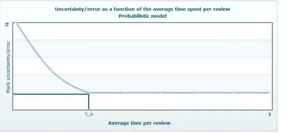
In the ideal case from a quality perspective, all reviewers read all contributions for as long as they need to take a decision, and contributions are as long as they need to be for the reviewers to fully grasp their value. With respect to the review time and contribution length, we assume in particular that as the review time and contribution length grow, the reviewer is able to narrow down the uncertainty/error on the review marks he or she wants to give. In other words, it will increase the confidence that the correct mark for the contribution is within a given interval. This is graphically depicted in Figure5 and6where we schematically plot the mark error function σras a function of time and
length respectively.
These schematic figures also show that beyond a certain time threshold trx and
length threshold lx the mark uncertainty remains constant. Reading a 10 pages paper
for 4 hours or 4 days is not likely to make a difference (if we are in doubt between giving a 6 and a 7 we will probably still be in doubt), but one minute versus four hours does.
In summary, the ideal process from a quality perspective is as follows:
– The number of reviews NR = NRC = |R| ∗ |C|, that is, the number of reviewers
Fig. 5: Given a constant effort, this is a possible model of the uncertainty of a review with respect to the average time spent by the reviewers
Fig. 6: Given a constant effort, this is a possible model of the uncertainty of a review with respect to the average length of the contributions
– The average time spent in reviewing tr= trx, where trxis the time that minimizes
the error in the review process;
– The contribution length lc = lx, where lxis the length that minimizes the error in
the review process (and the corresponding effort is tlx).
The reviewing effort is ER= trx∗ NRC. The writing effort is EW = tlx· NC
Informally, making the review process efficient requires reducing the effort mini-mizing the quality degradation. To this end we can act on the following parameters:
– the time devoted to each review or the length of the contribution (we assume the latter to be somewhat correlated to the writing effort);
– the number of reviewers per paper and the number of papers per reviewers; – the number of phases, with the aim of i) putting less effort on submissions that
are clearly good or clearly bad and more effort on borderline submissions, and ii) avoiding multi-phase processes that require update of the submission at each phase, if we recognize that having the extra phases is not beneficial to the process. We now see some metrics that we think will help us understand proper values for these parameters.
Reducing the number of reviews A line of investigation is around reducing the num-ber of reviews, and specifically reducing the numnum-ber of reviews for submissions whose fate is clear. This is the main reasons for having phases, where at each phase focus and effort is placed on the submissions for which a decision has not been taken yet. We consider now in particular the case in which the submission remains unchanged from a phase to the next (as in the Sigmod example discussed earlier).
Assume that the review process is structured in as many phases as the maximum number of reviewers per papers (say, we plan to have at most four reviews for a paper, so at most four phases). The analysis we want to make is to understand which is the earliest phase at which we can stop reviewing a given paper, because we have a sufficiently good approximation of the fate of the paper, which is the one we would get with the four reviews. In particular, given the number t of submissions we can accept (as long as they get marks above a minimal acceptance threshold), we want to estimate the earliest point (the minimum number of reviews) so that we can state whether a paper will or will not be in the top t. As an example, if a paper has two strong reject reviews, it is impossible for it to end up in the acceptance range, so we can stop the review process for this paper after two reviews. Similarly, if the paper has three rejects, we can confidently skip the fourth review. Stopping reviews for guaranteed acceptance is more complex as it depends also on the marks of other papers (being above a threshold is not enough as it is a competitive process) but essentially it always amounts to verify if there is a possible combination of marks for the missing reviews that can change the ranking to the point that the paper can end up in the reject bin.
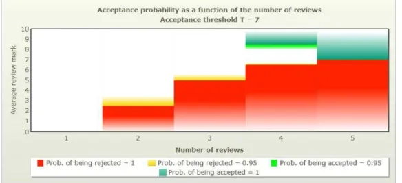
In Fig.7 we show the results of such deterministic approach for a specific case where |R| = 5, for each criteria Mjthe reviewer can assign a mark between {1, . . . , 10}
with no half-marks and with a acceptance threshold T = 7.0. The darker areas in the bottom of the diagram indicate the cases where the fate (rejection) of the contribution
is already finalized and no further review will change it. The shadow areas in the upper part indicate the symmetric cases where the acceptance of the contribution is sure, in this case that is based on a simple threshold.
Fig. 7: Deterministic acceptance and rejection of a contribution. The figure shows, given an average mark for r reviews, what is the probability that the contribution will be ac-cepted or rejected according to all the possible marks that could be given in the remain-ing |R| − r reviews
In addition to the deterministic analysis done above, which is conservative, we could perform a statistical analysis relying on the fact that reviewers’ marks should exhibit some correlation (if three reviewers give a weak reject mark, it is unlikely that the fourth will give a strong accept to bring the paper above the threshold). In general, after each phase, we can estimate the probability of each paper ending up in the accept or reject bin, and to do so we can also leverage our previous disagreement measures to help estimate the confidence associated to the estimate. This is also indicated in Fig.7only for explanatory purposes with the shadowed areas on top or below the deterministic rejection/acceptance areas.
Notice that implementing the above process requires either a multi-phase review, or requires giving reviewers a priority on what they should review so to increase the chances that the reviews they would have to do later may not be needed because the fate of the contributions has already been determined. The result of the analysis (the extension of the area that denotes when we can stop reviewing a paper) is informally described in the figure but is not formally described here. The formal analysis is part of our current research work.
Reducing the number of phases The goal here is to reduce the writing time by reduc-ing phases. It applies to processes where different phases require different submissions
(a la FET-Open). The metric we leverage is the Distance between rankings obtained
after different review phases. This metric is computed when a review process has
mul-tiple phases and contributions have to be ranked at the end of each phase according to the marks they got. The level of correlation can help to assess if, in a given review pro-cess, multiple phases with modified submissions are really needed. In order to measure this we use again the Kendall τ distance. In fact, the problem can be mapped to that of evaluating quality a posteriori, where we take the (supposedly more accurate) ranking after the second phase as a way to measure the quality of the results in the first phase. As in the quality case, we can only measure this for the contributions accepted after the first phase and that therefore went through the next phase.
The analysis of the distance between rankings may have a significant impact on reducing the effort. If the distance is high, then the two rankings are not correlated and one can question whether the first phase is significant at all. In this case, we would be rejecting many proposals that would get an excellent rank in the second phase. If the distance is low, then one phase is enough and we can spare the extra effort in writing and reviewing. Again, the formulation of a concrete suggestion for which values of Kendall should suggest to combine the phases is part of our current research.
Reducing the review criteria Another interesting dimension is the reduction of the criteria used for the review. The point here is not so much for papers - reviewers do not spend much time if they need to rate a paper with one, two or five criteria - but for project proposals. Specifically, in some cases proposals are evaluated along a set of criteria (e.g., impact on society) and authors have to write pages (spend effort) to demonstrate that their proposal satisfies the criteria. If we realize that certain criteria and associated marks are on average irrelevant for the final decision or can be predicted by looking at other marks, then we may decide to spare authors the related writing effort. To this end, we measure the Correlation between criteria, as correlation indicates the strength and direction of a linear relationship between two random variables. To assess the correlation between criteria we use the Pearson’s correlation factor:
Definition 16 (Pearson’s correlation factor). Let x and y be two random variables,
σxybe the covariance, σxand σybe the standard deviations, the Pearson’s correlation
factor is defined as follow:
ρxy= σxy
σxσy
(9)
with −1 ≤ ρxy≥ 1
Note that if:
– ρxy> 0, x and y are directly correlated, or positively correlated;
– ρxy= 0, x and y are independent;
– ρxy< 0, x and y are inversely correlated, or negatively correlated.
Therefore, if the Pearson’s correlation factor between two criteria x and y is ρ = 0, this means that the two criteria are independent, so it is useful to have both of them in the
review process, while if ρ = 1 then the two criteria are correlated, so it is useless to differentiate and it is better to group the criteria3.
As a variation, we can compute the kendall distance between the ranking of a spe-cific criterion and the final ranking, again to study which criterion is more significant for the final result. Again, the actionable part of this metric (the indication of which values should suggest combining marks) is under investigation.
Effort-invariant choices An additional line of investigation is around effort-invariant choices, that is, varying review process parameters to improve quality while keeping the effort constant.
Review time versus number of reviews. The first issue in this category that we
an-alyze is trading time spent on a review in exchange of an increase in the number of reviews. As we have seen before, the review effort is given by the time trspent
review-ing the contribution times the total number of reviews assigned NR:
tr=NERR
The trade off is between ranking a paper with few high quality (low uncertainty, as per the meaning defined above) reviews or many lower quality (more uncertain) reviews. Assuming that we can actually estimate, via surveys, the accuracy of the review based on time (on average, or for each reviewer), then we can identify which is the best trade-off.
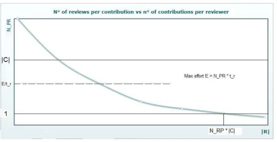
Committee size versus number of contributions per reviewer. A final effort-invariant
trade-off we consider is the size of the expert group versus the number of contributions each reviewer gets to review. We assume that effort E requested to each reviewer, av-erage time per review tr, and average preparation effort tware kept constant, and also
constant and decided a priori is the number NRPof reviews we wish to have for each
paper. We also assume that the number of submissions |C| is known or can be estimated. The number of papers or contributions per reviewer NP Ris equal to NRP|R|×|C|.
Fig-ure 8shows the plotting of this function, where NP R varies from a minimum value
of 1 (each reviewer gets one paper, which means that the size of the expert group is equal to the total number of reviews) to a maximum value of |C|. The question we try to address is what is the optimal point to be selected on the curve in the figure. In gen-eral, the point cannot be freely chosen because chairs typically decide the effort they can ask from each reviewer. This effort is defined by NP Rx trand depending on how
demanding chairs are, the corresponding line in the chart can be above or below the maximum value for NP R. Depending on the effort, therefore, NP Rcan vary between 1
and the smallest between |C| and E
tr, rounded to the lower integer. We refer to this value
as MP R(maximum number of papers per reviewer).
Given that all values of NP Rbetween 1 and MP Rare acceptable, the point is how to
fix this value - and consequently how to fix the size of the review committee. Intuitively, we believe that giving many papers per reviewer is preferable as the reviewer can form an opinion on the quality distribution of the papers and can mark them accordingly. If 3Incidentally, as a particular case, this metric could also be useful to assess quality if we find a high correlation between the reviewer confidence and the overall quality mark, e.g., we may find that reviewers with a low level of confidence always give low rate or high rate.
Fig. 8: Given a constant effort, a constant number of reviews and time per review, this is a possible model of the number of reviews per contribution with respect to the number of contributions assigned to each reviewer
a reviewer only sees one paper it may be hard to state whether this is good enough, and impossible to estimate if this is in the top k. The problem is particularly significant with junior reviewers who do not have an idea of the quality level to expect.
More quantitatively, there are two observations we make in this respect: the first is that high values of NP R are good because they allow us to detect biases. We have
more samples to make the case and determine if a reviewer has an accepting or rejecting behavior and possibly compensate. The second is that this raises the need for additional metrics to explore if there is a correlation between quality and NP R. Specifically, what
we propose is to compute the spread, agreement, robustness, and quality metrics for the various values of NP R in our datasets and examine if there is a correlation between
NP R and these metrics. We will perform this analysis in the following sections and
discuss conclusions and implications from the perspective of this metric.
3 Experiments on conference papers
3.1 Review process and dataset description
Metrics described in section2have been applied also to conference papers, adapting them to the different assessment procedure. This section presents the three datasets we use for the analysis, one related to a large conference (more than 500 submissions), another related to a medium-size conference (less than 500 submissions), and the third one related to a small workshop (less then 50 submissions) with predominantly young reviewers. All the datasets available refer to conferences in the ICT area. In the fol-lowing, for each dataset, we describe both the review process, basic information and statistics on the dataset and the computed metrics.
3.2 Large conference
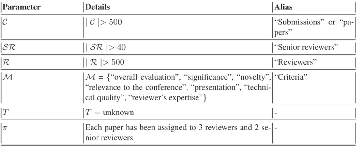
Parameter Details Alias
C | C |> 500 “Submissions” or
“pa-pers”
SR | SR |> 40 “Senior reviewers”
R | R |> 500 “Reviewers”
M M = {“overall evaluation”, “significance”, “novelty”,
“relevance to the conference”, “presentation”, “techni-cal quality”, “reviewer’s expertise”}
“Criteria”
T T = unknown
-π Each paper has been assigned to 3 reviewers and 2 se-nior reviewers
-Table 1: p = {C, E, M, T, π}
The conference covered topics related to computer science. Following our evalua-tion process model, we define the characteristics of the process in Table1. The number of papers per reviewer varies from 1 to 13 and the marks range from 0 (lowest) to 10 (highest), with no possibility of half-marks. The review procedure was the following: two program committee members (one primary and one secondary) and three reviewers have been assigned to each paper. Papers have been subject to blind peer review, so reviewers were not aware of the identities or affiliations of the authors. On average, we have 3 reviews per paper, and an overall set of more than 500 reviewers. A reviewer could also be an author of a submitted paper. The overall number of analyzed reviews is approximately 3000. After the peer review process, 20,7 % of papers have been ac-cepted.
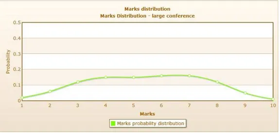
Fig.9shows the distribution of mark values, the majority of the values are con-centrated between 3 and 8. A lot of marks given by reviewers are very close to the acceptance threshold which ideally might have been between 5 and 6 (the exact value is not specified in the data set). The analysis is done considering only the first criterion (overall evaluation), which is the most important one to look at when deciding the fate (acceptance/rejection) of a paper.
Looking at Fig.9, the first thing we noticed is that the distribution is basically flat if we consider the values between 4 and 7. The expected value for the marks related to the first criterion is 5.4 and the standard deviation is 2.02.
3.3 Computation of quality-related metrics
Divergence a posteriori Here, we compute the divergence between the ranking of the conference and the ranking a posteriori given by the citation counts. We recall that
Fig. 9: Mark distribution for the overall evaluation criterion in the large conference
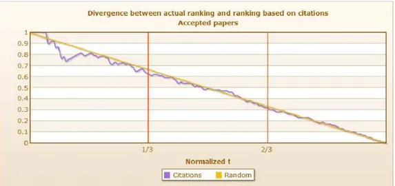
the conference was held in 2003, so we were able to compute how many citations the papers got in the subsequent years. We computed the divergence value only for the accepted papers, as only for these we have citations; indeed the rejected ones have not been published (at least not in the same version) so they did not get any citation. In Fig.10we highlight the divergence value for t=1/3A N Divρc,ρa(1/3A, A, A) = 0.63
and t=2/3A N Divρc,ρa(2/3A, A, A) = 0.32 4.
The former value means that by looking at the top 1/3 of the papers in the two rankings, 63% of these papers differ. If - and this is again an assumption that is not proven - we extend the reasoning to all papers instead of considering only the top 1/3, this means that in a process that accepts 1/3 of the submissions, the review process and the random selection process have the same quality in approximating the citation-based ranking. For completeness, we also compute the value of the Kendall τ distance among the two rankings, the normalized value is N Ktau = 0.49. We recall that a
value N Ktau = 0 means that the papers are in the same order, while N Ktau = 1
means that no one of the papers is in the same position w.r.t the two rankings. The value
N Ktau= 0.49 confirms again our previous result (based on the divergence metric) that
the review process of such a conference has performed poorly w.r.t. the citation-based count, therefore papers that were ranked very good in the conference got less citations of papers that were lower in the ranking, and that happened for almost 50% of papers. Disagreement between reviewers Following definitions in Section2.2we have com-puted the average disagreements between reviewers and we report the results of the computation in Fig. 11. In order to compare the different conference dataset among 4We indicate with A the number of accepted papers, which we recall was 20.7% of total
Fig. 10: Normalized divergence calculated for accepted papers
themselves, all values in this section are normalized (i.e. divided by the highest possi-ble value: maximum disagreement, maximum bias, etc..).
Here, the values computed for the disagreement are not surprising: the disagreement computed with the actual data is consistently lower than the random one, and lower than the one computed with the reshuffling of the marks. Such a straight difference could be due to the fact that here the reviewers use consistently the entire scale, so marks assigned to the papers are, at the end, more distributed.
Then we also computed the average disagreement w.r.t. the number of reviews done and we have not found any particular correlation.
Robustness In order to assess the impact of a perturbation on the mark values and find how this can affects the number of accepted/rejected papers we compute the robustness of the process. We applied a perturbation of ² = 1, meaning that we randomly selected among three possible variations of the marks: -1/0/1. Note that we apply a stochastic variation to each one of the six marks. Then we compute the divergence between the actual ranking and the ”perturbated” one, computed as already explained in Section 2.2. In Fig.12are shown results for t=A, that is the number of accepted papers. The divergence value is only N Divρa,ρ²(A, C, C) = 0.06
5. This is a very low value, as a
perturbation in the mark value of ² = 1 impacts only the 6% of the papers. Summing up, the analysis of these data suggests that the process is quite robust.
(a) Average disagreement Ψ and standard error σ
(b) Average disagreement γ and standard error σ computed sepa-rately for reviewers grouped by number of reviews made
Fig. 11: Computed average disagreement
Fairness-related metrics The same metrics used in the project analysis has been ex-ploited for papers. Here, we only changed the threshold fixed to determine if a reviewer is biased or not. In this case we only consider reviewers who assessed at least 4 papers, with an average bias greater than 1 for the positive case and lower than −1 for the neg-ative case (please remember that in this data set, ±1 is the minimum marks difference). The obtained results are collected in Fig.13and Fig.14. As previously said, the dis-agreement and the bias values have been computed using the metrics defined in Section 2.2.
Reviewers with ID=796 and ID=347 (Fig.13) have given higher marks than the others on more than 10 papers. In particular, their marks have been more than one point higher, on all the criteria, with respect to the average of the marks given by the other reviewers to the same paper. Remarkable is the case of the reviewer with ID=1461 (see Fig.13), who, despite the low number of reviews he made, has given marks that are almost 3.5 points higher on every criterion than those given by the other reviewers. Quite interesting is also the case of the reviewer with ID=2497 (see Fig.14), who gave marks that are more than 2 points lower on every criterion than those given by the others.
We perform a simple unbiasing procedure: considering only reviewers having a bias greater than 1, we add or subtract the individual computed bias in order to obtain a new ”unbiased” rank. Finally, we compute the divergence between the two rankings, the biased and the ”unbiased” one, obtaining N Divρ1,ρ2(A, C, C) = 0.09. The divergence
value is computed for the accepted papers, the result means that the 9% of the papers could be affected by the unbiasing procedure. As the 0.09 value is greater then the one computed for the minimal stochastic variation (0.06), the ”unbiased” procedure could have a real effect in this case, if the conference chair would decide to use it.
3.4 Computation of efficiency-related metrics
Correlation between criteria In Fig.15we have reported the correlation computed between each pair of criteria. The first criterion (“Overall evaluation”) is the overall judgment for a given paper. Through the calculation of Pearson’s correlation coefficient it has been found that the overall acceptance of a paper strongly depends on three core features: the significance of the paper, its novelty and its technical quality. The paper relevance to the conference and also the presentation do not have the same importance with respect to the paper acceptance.
Fig. 15: Correlation between criteria
Another aspect came out from the analysis of the correlation: the confidence score, in general, is not correlated with the other criteria. This is coherent with the fact that conceptually the quality of the proposal is independent from the expertise of the re-viewer in the research field.
3.5 Medium-size conference
The second conference dataset we analyze refers to a medium-size conference held in 2008, with more than 200 submissions, more than 100 reviewers, no senior reviewers, with only one criterion to decide the overall evaluation of the paper. The mark scale ranges from 1 to 7, with no half marks. No threshold was defined, each paper was assigned to 3 or 4 reviewers and the peer review process was blind. The number of reviews analyzed is more than 800. The acceptance rate of the conference was 18%. The peer review process is summarized in Table2.
Fig. 16shows the mark distribution. It is interesting to note that the most frequent marks is 2, and that there is a low probability to get a mark in the middle of the scale (4 in this case).
Parameter Details Alias
C | C |> 200 “Papers”
SR | SR |= 0 “Senior reviewers”
R | R |> 100 “Reviewers”
M M ={”overall evaluation”} “Criteria”
T T = undefined
-π Each paper has been assigned to 3 or 4 reviewers
-Table 2: p = {C, E, M, T, π}