An eclectic third generation model of financial and exchange rate crises

DOCUMENTS DE TREBALL

DE LA FACULTAT DE CIÈNCIES

ECONÒMIQUES I EMPRESARIALS

Col·lecció d’Economia

E08/196

An eclectic third generation model

of financial and exchange rate crises

Joaquín Novella Izquierdo

Universitat de Barcelona

Joan Ripoll i Alcón

Escola d’Estudis Empresarials del Maresme

Adreça correspondència:

Departament de Política Econòmica i Estructura Econòmica Mundial Facultat de Ciències Econòmiques i Empresarials

Universitat de Barcelona. Avda. Diagonal, 690 Torre 6, 3ª planta, despatx 6334

08034, Barcelona (Spain) telèfon: 934029000

Abstract: This paper presents an eclectic model that systematizes the dynamics of

self-fulfilling crises, using the main aspects of the three typologies of third generation models,

to describe the stylized facts that hasten the withdrawal of a pegged exchange rate system. The most striking contributions are the implications for economic policy as well the vanishing role of exchange rate as an instrument of macroeconomic adjustment, when

balance-sheet effects are a real possibility.

JEL Classification: E44, E52, F31, F32, F34, F36, F41, F43

Keywords: financial and exchange rate crisis, speculative attack, financial panic, financial liberalization

Resum: En aquest treball es presenta un model eclèctic que sistematitza la dinàmica de les crisis que “s’autoconfimen”, usant els principals aspectes de les tres tipologies dels models de crisis canviàries de “tercera generació”, amb la finalitat de descriure els fets que precipiten la renúncia al manteniment d’una paritat fixada. Les contribucions més notables són les implicacions per a la política econòmica, així com la pèrdua del paper del tipus de canvi com instrument d’ajust macroeconòmic, quan els “efectes de balanç” són una possibilitat real.

Paraules clau: crisis financeres i de tipus de canvi, atac especulatiu, pànic financer, liberalització financera

INTRODUCTION

The worldwide financial integration characteristic of 1990s has contributed strikingly to increase the frequency and the intensity of exchange rate crises in emerging countries. As a result, over the last fifteen years, it has been flourishing studies, both theoretical and empirical, about the nature and causes of the withdrawal of pegged exchange rate systems. Despite we could identify large common features in these different crises episodes, today there isn’t yet a canonical model of financial and exchange rate crises in economic literature. In fact, when Eichengreen, Rose and Wyploz (1995) introduced the terminologies of first and

second generation crisis models, they were pointing up that every new wave of crises was

giving rise to a new typology of interpretative schemes.

Thus first generation models were the explanation of exchange rate crises at the beginning of 1970s, whereas inspiration to second generation models arose from the string of speculative attacks that the Exchange Rate Mechanism (ERM) of European Monetary System (EMS) suffered between 1992 and 1993 as well as the Mexican crisis in 1994. Again, the proliferation of third generation models was the result of efforts to analyze the East Asian crisis in 1997.

This lack of consensus about the nature of modern exchange rate crises makes it difficult to identify the factors that have caused them. In this way, Krugman (2000) wrote “if we can’t

agree about what happened, how we can blame increasing foreign trade or another factor of the collapse of exchange rate system?”

Nevertheless, since the burst of the 1997 East Asian crisis, there was a definitive tendency in economic literature to move away from models that emphasized moral hazard problems in benefit of some self-fulfilling panic. At the same time, this self-fulfilling panic was increasingly related to maturity mismatches and/ or currency mismatches.

For this reason, it would appear to be a good moment, today, ten years after the East Asian crisis, to present an eclectic model that synthesizes the different versions of the third

generation exchange rate crises models, and describes stylized facts that hasten the

withdrawal of a pegged exchange rate system.

The paper is divided into four parts and one appendix. In the first one, the different variants of

third generation exchange rate crises models are presented. In the second section, we create

an eclectic model that systematizes the dynamics of self-fulfilling crises, focusing the main aspects of the three typologies of third generation models. The third part describes, drawing on the model built previously, the stylized facts that hastened the financial crisis and pegged

exchange rate system withdrawal. The final section summarizes the main results find out while annex offers some empirical evidences that reinforces all our arguments.

1. THE LOGIC OF THIRD GENERATION MODELS

After the burst of the Eastern Asian financial and exchange rate crisis in the summer of 1997, many analysts pointed out that the concepts and models prevailing at that moment didn’t fit with the dynamic of crisis and misinterpreted data1. An then, likewise the Exchange Rate Mechanism crisis of EMS in 1992 and later the Mexican Crisis at the end of 1994 raised doubts about classic models, the Asian crisis questioned explanatory power of second

generation models and speed up the appearance of new interpretative schemes, which by

taking aspects of traditional models, provided relevant factors to analyze a new typology of exchange rate crisis. So these new models became, in their early stages, a synthesis approach that tried to mix the main characteristics of the first and second generation models to explain the causes of the 1997 East Asian crisis. However, the evolution of this new wave of models ended up shaping a third generation with their own identity.

The third generation crisis models revolve around three basic variants. A first version of these models implies a string of investments affected by moral hazard that leads to an excessive growth of foreign debt and afterwards to the collapse of financial and exchange rate system. This story has its origin in McKinnon and Pill’s (1996) article, taken up later by Krugman (1998) and developed in-depth by Corsetti, Pesenti and Roubini (1999). A second version, complementary to the previous one and linked above all to Chang and Velasco (1998a and 1998b), is created around Diamond and Dybvig’s (1983) bankruptcy model applied to an open economy. Finally, the third version analyzes how financial difficulties, which are associated to national currency devaluation, undermine domestic companies’ solvency and macroeconomic fundamentals. This last argument is claimed to Krugman (1999b and 1999d) as well as Schneider and Tornell (2000).

1 _{See Corsetti (1998), Corsetti, Penseti and Roubini (1998), Calvo (1998), Calvo and Végh (1998), Cavallari and Corsetti (1996) and Flood}

2. AN ECLECTIC THIRD GENERATION MODEL

At this point, we introduce an eclectic model that systematizes the dynamics of self-fulfilling

crises, from the consideration of main aspects of the three variants of third generation models.

Our analysis implies three basic equations and two functions that allow us to describe the gestations and bursting of a financial and exchange rate crisis as well as the significance of the balance sheet problems and their devastating effects.

2.1. THE SPECIFICATION OF THE MODEL

2.1.1. GOODS AND SERVICES MARKETS: THE REAL ECONOMY (RE) CURVE The first equation of the model reproduces the working of goods and services markets. As we know national output (Y) equals to aggregate demand (AD) in equilibrium.

(1) Y≡AD=C+I+G+X−M

We can breakdown the former equation using the components of aggregate demand (AD) that is the sum of Consumption (C), Investment (I), Government Spending (G), and Exports (X) minus Imports (M). Let’s now discuss each of these five components in turn.

Private Consumption depends on disposable income (YD) and on domestic interest rates. Then we write Private Consumption function as follows:

0 ; 0 < ∂ ∂ > ∂ ∂ r C YD C (1a) C=C+c₁⋅YD−c₂⋅r ,

As we can see the relation between Private Consumption, disposable income and domestic interest rates is characterized by two parameters: c1 and c2. The parameter c1 is the propensity

to consume whereas c2 is the sensitivity of consumption to changing interest rates. It seems

logical to think a natural restriction on c is that it will be positive and on c1 2 is that it will be

negative. Thus, consumption demand is positively related to disposable income and negatively related to national interest rates. On the other hand, C represents autonomous consumption, which is economy’s minimal consumption, essential to cover basic consumption needs.

(

Y tY TR

)

c r c C C= + ₁⋅ − + − ₂⋅ 0 0 <0 ∂ ∂ < ∂ ∂ > ∂ ∂ r C ; t C ; Y C (1a.1) ,

We suppose disposable income is given by YD = Y – T + TR, where Y is domestic income, T is income taxes paid taxpayers and TR is Government transfers received by consumers. In addition, we assume T = t·Y, that is taxes are a proportional tax on income. Higher taxes decrease consumption, also less than one for one. We will also take transfers TR =TR as an

exogenous variable. Then, equation 1a.1 tells us that consumption is a function of income, taxes and domestic interest rates.

Private Investment is a function of domestic interest rates (r) and companies’ self-finance capacity (SFC). I is the autonomous investment and symbolizes economy’s minimal investment. 0 ; 0 < ∂ ∂ > ∂ ∂ r I SFC I r b SFC b I I = + 1⋅ − 2⋅ (1b) ,

The relation of Private Investment with national interest rates and companies’ self-finance capacity (SFC) depends on two coefficients: b1 and b . The b2 1 coefficient is the propensity to

investment related to SFC. Its value will be positive because the higher companies’ self-finance capacity (SFC) the higher companies’ investment. The coefficient b2 is the sensitivity

of investment to changing interest rates and its value is negative. This parameter collects companies’ expectations.

Here, we suppose that companies’ self-finance capacity depends on equity value, the difference between assets (A) and debt value. Debt value is the sum of domestic debt (D) and foreign debt in local currency (E·D*). As we are thinking in terms of emerging countries, we consider there is an ”original sin” problem2 so national companies can borrow abroad but they only invest in national assets.

Consequently, equation 1b can be written as 1b.1:

0 ; 0 < ∂ ∂ < ∂ ∂ E I r I

(

)

[

A D E D

]

b r b I I = + ⋅ − + ⋅ * − ₂⋅ 1 (1b.1) ,

[

_{Assets Debt}

]

_A

(

_{D E D}*

)

Equity SFC = = − = − + ⋅ where

Thus, any nominal exchange rate depreciation drives up foreign debt value in national currency, and it defines a negative causality between private investment and nominal exchange rate movements.

2_{Original sin shows how the existence of incomplete capital markets makes it difficult for the emerging economies’ ability to issue debt in}

international bond markets, an extreme that forces them to get into foreign currency debt in order to capture external saving and this puts the national economy at currency risk.

The third component of demand in our model is Government spending. We will take G as an exogenous variable because, thought Government behaviour is predictable, we will suppose there isn’t a reliable rule we can write for it.

G

G=

(1c)

Exports are the part of foreign demand that falls on domestic demand. They depend on foreign income in nominal terms (p*·Y*) positively because, ceteris paribus, higher foreign income means higher foreign demand for all goods and services. So, higher foreign income leads to higher exports. In the same way, exports also depend on nominal exchange rate (E). The higher the nominal exchange rates, the higher foreign demand for domestic goods, and, the higher exports. Finally, the x1 parameter gauges economy’s trade openness. X represents

autonomous exports. 0 ; 0 * _∂ > ∂ > ∂ ∂ E X Y X (1d) * * , 1 E p Y x X X = + ⋅ ⋅

Imports are the part of domestic demand that falls on foreign goods and services. They depend on domestic income in nominal terms (p·Y) negatively because, ceteris paribus, higher domestic income means higher domestic demand for all goods and services, both domestic and foreign. So, higher domestic income leads to higher imports. Thus, the propensity to import illustrated by the m1 parameter is negative.M represents autonomous

imports. Finally, even though imports also depend on nominal exchange rate (E) negatively3, we don’t consider it explicitly because we show imports in terms of domestic currency.

0 1> = ∂ ∂ m Y M , (1d) M = M + m₁ ⋅ p ⋅Y

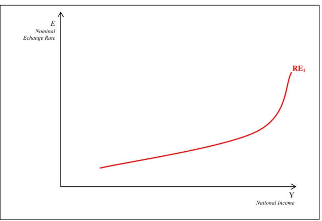
Putting all these components together, we can construct the RE curve illustrated in figure 1. It plots the functioning of a country’s real economy.

The RE curve is really a function formed by all combinations of nominal exchange rates (E) and domestic output (Y) for which markets of goods and services are in short-term equilibrium. It means aggregate output equals to aggregate demand, as expression 1e shows.

(

)

(

) (

)

[

*

]

1 * * 1 1 2 2 ) (c b r b A D x E p Y b E D S Y =α − + ⋅ + ⋅ − + ⋅ ⋅ ⋅ − ⋅ ⋅ (1e) RE Function → 1 1 1 1 1 m t c c + ⋅ + − =

α is the autonomous spending multiplier where

[

C I c TR G X M

]

S= + + ₁⋅ + + − is the autonomous spending and

Figure 1. Goods and services markets operation: Real Economy (RE) curve

Source: Author’s own diagram based on Krugman (2000)

Assuming fixed price levels at home and abroad in the short-term and no foreign debt (D*=0),

the previous RE function can be written as:

(1e.1) RE1 Function → Y=α

[

S−(c2 +b2)⋅r+b1⋅

(

A−D

)

+

(

x1⋅E⋅p*⋅Y*

)

]

Here, a rise in nominal exchange rate makes foreign goods and services more expensive relative to domestic goods and services. So, this relative price change caused by nominal depreciation increases domestic goods competitiveness, fostering higher exports. A larger foreign demand explains the rising in aggregate demand that stimulates domestic output growth.

From these arguments we can deduce a positive relation between nominal exchange rate and national income that we will call pro-competitive effect and which is gathered through

(

* *

)

1 E p Y x ⋅ ⋅ in expression (1e). Pro-competitive effect: * * 0 1⋅ > = ∂ ∂ Y p x E Y

For the moment, this pro-competitive effect explains the positive slope of RE1 curve in figure 1.

3_{The higher the nominal exchange rates the lower domestic demand for foreign goods, so they are more expensive and imports will go down}

E Nominal Echange Rate RE1 Y National Income

2.1.2. MONEY MARKET AND FOREIGN EXCHANGE MARKET: THE FINANCIAL ECONOMY (FE) CURVE

The second of equations that forms this eclectic model that we are building, represents national money market equilibrium.

P M P Md S = (2) ⎟⎟ ⎠ ⎞ ⎜⎜ ⎝ ⎛ P MD

The real money demand is the total demand for money in real terms for all households and companies in the economy. We write money demand in real terms as a function of nominal interest rates (r) and domestic income (Y).

0 ; 0 < ∂ ∂ > ∂ ∂ r M Y Md d

( )

Y r lY l r L P Md ⋅ − = = , _{1 2} (2a) ,

As we can see the relation between real money demand, domestic income and national interest rates is characterized by two parameters: l and l1 2. The parameter l1 is the sensitivity

of demand for money to changing domestic income and collects money demand for transaction and precaution reasons. l1 has a positive value because demand for money will

increase in proportion to nominal income.

On the other hand, the parameter l2 is the sensitivity of money demand to changing interest

rates and shows the function of money as store of value. It seems logical to think a natural restriction on l2 is that it will be negative because the higher interest rate the higher the

opportunity cost of money holdings.

⎟⎟ ⎠ ⎞ ⎜⎜ ⎝ ⎛ P MS

The money supply in real terms gauges purchasing power of the amount of money (MS) in economy. We suppose money supply in real terms depends on monetary base (H) and money multiplier (mm). H mm P MS ⋅ = 0 ; >0 ∂ ∂ > ∂ ∂ H M mm MS S (2b) ,

Let H monetary base that is the supply of central bank money. We assume H is directly controlled by central bank as well as it can change the amount of H through open market operations. So, the higher monetary base, the higher money supply.

At the same time, the effectiveness of open market operations depends on money multiplier

mm. It implies that a given change in monetary base (H) has a larger effect on the money

Obviously, given price level (P), equilibrium in financial markets requires that real money demand _⎟⎟ ⎠ ⎞ ⎜⎜ ⎝ ⎛ P MD ⎟⎟ ⎠ ⎞ ⎜⎜ ⎝ ⎛ P MS

be equal to money supply in real terms .

(

)

P M H mm r l Y l P Md S = ⋅ = ⋅ − ⋅ = _{1 2} (2b)

And rewriting this previous equation 2b, we find the equilibrium domestic interest rate:

(

)

Y l l H mm l r=− ⋅ ⋅ + ⋅ 2 1 2 1 0 ; 0 < ∂ ∂ > ∂ ∂ H r Y r (2c) , 4

Related to this, we suppose that the fear of floating moves central bank to compensate any change of nominal exchange rate. In order to collect this subordination of monetary policy to the maintenance of certain parity, we introduce the third of the model equations: interest rate parity condition in presence of imperfectly substitute financial assets. Interest parity condition states that foreign exchange rate market is in equilibrium only when expected rates of return on domestic and foreign currency deposits plus a premium risk (ρ) –which reflects the spread between national and foreign bonds risk– are equal.

(3a) r=r* +d+ρ

In this way domestic interest rates (r) gauge expected rate of return on financial investment in domestic currency deposits (RFIDC). Likewise, the sum of foreign interest rates (r*) plus depreciation rate (d) is expected rate of return on financial investment in foreign currency deposits (RFIFC).

For a given expected future exchange rate (EE) and premium risk (ρ), the interest rate parity condition describing foreign exchange market equilibrium –in presence of imperfectly substitute financial assets– is the equation 3a:

ρ + ⎟⎟ ⎠ ⎞ ⎜⎜ ⎝ ⎛ − + = E E E r r * E E E E d E ₋ = 0 ; 0 * > ∂ ∂ < ∂ ∂ r E r E (3b) , where and

We found the equilibrium domestic interest rate in equation 2c. Now, we replace it in equation 3b to get 3c.

(

)

Y r l l H mm l E E E r r E = ⋅ + ⋅ ⋅ − = ρ + ⎟⎟ ⎠ ⎞ ⎜⎜ ⎝ ⎛ − + = 2 1 2 * 1 (3c)

4_{Calvo and Reinhart (2000) define fear of floating as emerging economies reluctance to allow exchange rate free floating. This extreme}

And if we try to isolate the monetary base (H), expression 3c turns into 3d. ⎟⎟ ⎠ ⎞ ⎜⎜ ⎝ ⎛ ρ + − + ⋅ − = E E E r mm l Y mm l H 1 2 * E _{0; <0} ∂ ∂ < ∂ ∂ E M E H S (3d) ,

Equation 3d shows clearly monetary policy subordination to the maintenance of certain parity. It means exchange rate and money supply will evolve in opposite directions. If there is a depreciation tendency, central bank will be forced to intervene in foreign exchange markets, selling foreign currency in exchange for domestic currency. This action will reduce international reserves endowment as well as monetary base and money supply. On the contrary, pressures for appreciating domestic currency will force central bank to buy foreign currencies, which will help to widen monetary base.

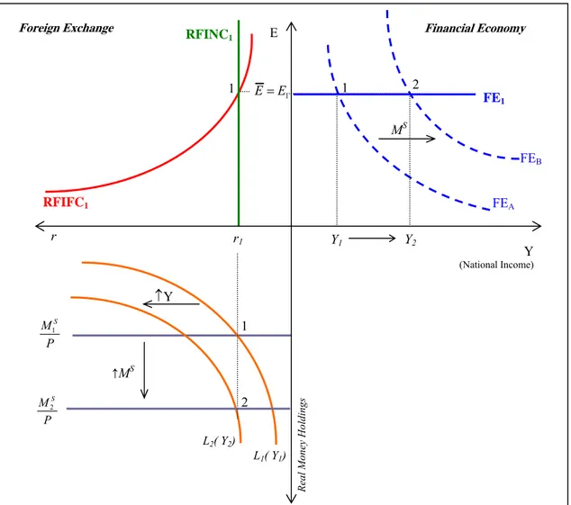
Figure 2. National money and foreign exchange market: FE curve if central bank does not intervene r2 r1 2 ↑Y 1 L2( Y2) _L 1( Y1) National Money Market

2 P MS 1 r _{Y1 Y2} Foreign Exchange E2 E1 RFINC1 RFINC2 1 2 R

eal Money Holdings

Y (National Income) E _{Financial Economy} 1 FE RFIFC1

Note: Out of convenience, the graph where foreign exchange market is drawing has been rotated 90° anti clockwise, in a way that interest rates is rising when they are moving to left side in x-axis meanwhile in y-axis exchange rate increase as further up in the axis. Analogously, the graph which illustrates national money market has been rotated 270° clockwise, thus real money holdings are gauged from coordinate origin downward on the vertical axis, whereas interest rates are measured from coordinate origin towards right side on the x-axis.

Source: Author’s own diagram.

Putting all these components together, we can build the FE1 curve illustrated in figure 2. It plots the functioning of domestic and foreign financial markets. In this way, the FE1 curve is a function formed by the combinations of nominal exchange rates and national output for which national money market and foreign exchange market are in equilibrium simultaneously. Mathematically, reordering equation 3d and isolating E or Y, we can define the Financial

Economy (FE) function in terms of equilibrium exchange rate:

(

)

_⎟⎟− −ρ ⎠ ⎞ ⎜⎜ ⎝ ⎛ ⋅ + ⋅ ⋅ − + = * 2 1 2 1 1 Y r l l H mm l E E E 0 < ∂ ∂ Y E (3e) FE Function → ,

or the Financial Economy (FE) function in terms of equilibrium output:

(

)

_⎟⎟ ⎠ ⎞ ⎜⎜ ⎝ ⎛ ρ + − + ⋅ + ⋅ ⋅ = E E E r l l H mm l Y * E 1 2 1 1 0 EY < ∂ ∂ (3e.1) FE Function → ,

FE curve determines an inverse causality between national output and nominal exchange rate, plotted in upper right panel in figure 2.

Nevertheless, the model that we are creating assumes that central bank is committed to exchange rate stability.

Let us suppose, there is rise in output from Y up to Y1 2 that causes an increase of money demand for transaction reasons, which graphically shifts money demand curve L1 towards the left side in lower left panel in figure 2.

If money supply doesn’t change, an excess of demand will occur in national money markets raising national interest from i as far as i1 2. It enhances the rate of return on financial investments in domestic currency deposits (from RFINC up to RFINC1 2), giving rise to a capital inflow that will hasten a local currency appreciation from E to E1 2, if central bank doesn’t intervene in foreign exchange markets.

But this is not the case. The subordination of monetary policy to the maintenance of certain parity5 will force central to intervene in foreign exchange markets to avoid domestic currency

appreciation. In this scenario, monetary authority must buy foreign currency, widening monetary base and money supply in real terms, in absence of sterilization.

P Ms 1 P Ms 2

Graphically, it causes a scrolling down of function as far as in lower left panel in figure 3 and FEA curve towards right side as far as FE in the top panel. B

Figure 3. National money and foreign exchange markets: FE curve if central bank intervenes

Source: Author’s own diagram.

In this way, central bank’s performance achieves to compensate exchange rate downward tendency as well as national interest and capital inflows rising. Consequently, the exchange rate parity will remain constant in E1 in spite of higher output. It means that if there are international reserves enough expected exchange rate equals equilibrium exchange rate (EE=E1) an then FE function becomes a FE1 curve completely elastic.

(3e.2) FE1 Function → = ⋅

(

⋅

)

+ ⋅

(

r* +ρ

)

l l H mm l Y 1 2 1 1 , =0 ∂ ∂ Y E RFINC1 1 RFIFC1 MS E 1 L2( Y2) L1( Y1) 2 1 ↑Y ↑MS P MS 1 P MS 2 Y1 2 Y2 r1 1 E E= FEA FEB R

eal Money Holdings

Y

(National Income)

r

Foreign Exchange Financial Economy

3. THE DYNAMICS OF THIRD GENERATION CRISES 3.1. THE ORIGINS OF FINANCIAL FRAGILITY

Using the model developed in the previous section, we can collect the logic of financial and exchange rate crises explained in the different types of third generation models to describe 1997 East Asian crisis.

With this aim, we consider the case of Sintaiko. Sintaiko is an imaginary emerging market economy defined as a country with low-to-middle per capita income of East Asian.

Sintaiko’s exchange rate policy is articulated on the basis of a pegged exchange rate system. The election of this kind of regime is explained by policymakers wish to stabilize trade flows in a country where the most operations are denominated in foreign currency; but also responds to the idea of using the exchange rate as a nominal anchor. This practice reduces the central bank’s independence but, at the same time, offers a credible rule for the monetary policy formulation that allows escaping from temporarily inconsistent actions. Likewise, the central bank fixes currency parity in an E1 value.

Figure 4 combines the RE and FE functions to determine the macroeconomic short-term equilibrium. Sintaiko’s economy will only be in equilibrium when the markets of goods and services and the financial markets –both national money and foreign exchange markets– are in balance simultaneously.

In this way, equations (1e.1) and (3e.1) establish that for any level of national output (Y), there is a nominal exchange rate value (E) that satisfies the interest rate parity condition – given real money supply, foreign interest rates (i*), expected exchange rate (Ee), premium risk (ρ) and domestic (P) and foreign price (P*) levels–.

This situation, graphically, will take place at a point like 1, where the intersection of RE1 and FE curves determine an equilibrium nominal exchange rate E1 1 and a national income Y1. If we assume that equilibrium parity (E1) coincides, circumstantially, with exchange rate fixed by central bank ( E =E1) and with future expected exchange rate (EE), the initial FE1A curve is transformed into the FE1B curve (a completely horizontal function), because depreciation expectations will be void (d=0).

Point 1 describes Normal Equilibrium (Krugman, 2000), where equilibrium output equals to: = ⋅

(

⋅

)

+ ⋅

(

_r* +ρ l l H mm l Y 1 2 1 1 1

)

and equilibrium exchange rate matches up with exchange rate fixed by central bank ( E =E1) as well as with the future expected exchange rate (EE). In addition, we are assuming fixed price levels at home and abroad in the short-term and no foreign debt (D*_=0).

Figure 4. Sintaiko’s Eonomy Short-Tem Equilibrium

E

Source: Author’s Own Diagram.

At this scenario, the successful economic development strategy based on export promotion, implemented over the previous decades, moves Syntaiko to integrate further in global capital markets, taking into account several international financial agencies’ advice. In this way, in a favourable momentum, economic authorities decide to remove capital controls and accelerate the liberalization of domestic financial markets.

The removal of financial restrictions that limit capital mobility, in a context of continual domestic growth and foreign interest rates abnormally low6, give rise to a huge increase in investment inflows. Although part of them takes the form of foreign direct investment (FDI), most of these capital inflows are short-term credits in foreign currency.

This is driven not just the inability of Sintaiko’s companies to obtain mid- long funds in narrow-shallow domestic capital markets (original sin), but also because the pegged exchange rate system makes exchange rate risk less perceptible. This short-term indebtedness in foreign currency is reinforced by implied guarantees over companies’ investments on behalf of Sintaiko’s Government –introducing a moral hazard problem– as well as by poor regulated financial institutions.

Then, Sintaiko is involved in an unstoppable dynamics of increasing foreign indebtedness that turns the country into an extraordinarily vulnerable economy to a financial panic situation for three main reasons.

6_{We are assuming there is a liquidity excess in capital markets of advanced economies.}

RE1 Y1 E = E1 FE1 (EE=E1) 1 Nominal Exchange Rate Y National Income Normal Equilibriu

First, in a context of free capital mobility, the lack of well-developed mid-long term capital markets confers commercial banks a pre-eminent role as financial intermediaries and accounts for “hot money” arising arranged in short-term or very short-term credits, loans and deposits that increase the likelihood of sudden stop in these capital inflows, in the face of any unexpected event that changes future expectations.

Second, the faults in domestic capital markets moves domestic companies to finance their long-term investments by means of short-term debt in foreign currency because, on the one hand, expected benefits on long-term investment offset the possible liquidity problems stemming from short-term financing; and, on other hand, the advantages of getting into debt abroad at low interest rates prevailing over potential costs of possible domestic currency devaluation, even more when the pegged parity is seemingly credible and there is an implicit warranty of bailing-out bad investments.

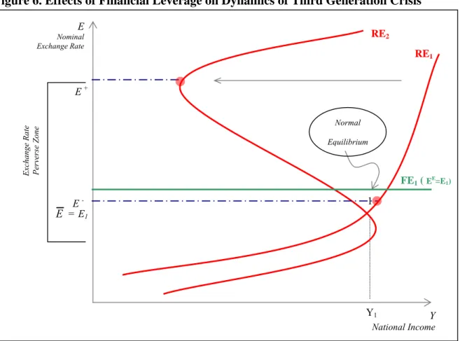
This tendency to progressive short-term financial leverage in foreign currency, graphically, entails a gradual curvature backwards of RE original curve that transforms it into RE1 2 curve in figure 5 and 6.

This is because the real effects of devaluation can change when financial and non financial national companies have too much foreign currency short-termed debt. Maturity mismatches as well as currency mismatches7 generate a latent problem in companies' balance-sheets that could compromise their solvency if a sudden capital flight or devaluation happens.

In this way, when domestic companies are very short-term leveraged in foreign currency, their financial position will be notably vulnerable, because possible national currency devaluation will reduce expected rate of return on investments in domestic currency and will increase the value of foreign currency debits in terms of domestic currency.

This extreme undermines companies’ net asset value, generates liquidity problems and diminishes their investment capacity8. This inverse causality between nominal exchange rates and national output is called balance-sheet effect –balance-sheet problems in the terminology of Krugman’s 1999 and 2000– and explains private investment shortfalls that reduce domestic demand and affect economic activity negatively. Again, expression (1e) catches up this

Balance-sheet effect by means of

(

*

)

2 E D b ⋅ ⋅ . 0 * 2 ⋅ < = ∂ ∂ D b E Y Balance-Sheet Effect:

7_{A currency mismatch arises from an asynchrony between currency in which debts are called and currency in which investments are made.}

A maturity mismatch occurs when domestic companies finance long-term investment projects with short-term credits.

8_{When companies are much leveraged, their indebtedness capacity is practically void and, then, financing new investment is diminished to}

But, when economic downturn caused by those financial difficulties is important enough, the

balance-sheet effect and, by extension, domestic currency devaluation will have recessive

effects on real economy, leading to RE1 curve in figure 1 bows backwards and changes into RE . 2

(

)

(

) (

)

[

_{S (c b ) r b A D x E p}* _Y* _{b E D}*

]

Y=α − ₂ + ₂ ⋅ + ₁⋅ − + ₁⋅ ⋅ ⋅ − ₁⋅ ⋅

(1e.2) RE

Exchange Rate Per

ver

se Z

one

2 Function →

We assume that this singularity applies for nominal exchange rate values ranged between E− and E+. This interval determines a perverse zone (PZ) for which the balance-sheet effect overcomes the pro-competitive effect. Here any nominal devaluation –given the impact on companies’ balance-sheet– loses their role as instrument of macroeconomic adjustment and it becomes a clear damage for the economy. Mathematically,

(

) (

)

[

*

]

0 2 * * 1⋅ − ⋅ < = ∂ ∂ D b Y p x E Y * * 1 * 2 D x p Y b E E E+ ≥ ≥ − ⇒ ⋅ > ⋅ If and then,

Graphically, this relation is represented by the downward-sloping RE2 between E− and E+. Figure 5. Goods and services markets operation: Real Economy (RE) curve

Source: Author’s own diagram based on Krugman (2000)

However, for nominal exchange rate levels lower than E−and higher than E+, the RE2 curve keeps its original upward slope.

E Nominal Echange Rate

RE1

RE

Pro-Competitive Effect> Balance Sheet Effect 2

Y National Income E +

E - Balance Sheet Effect > Pro-Competitive Effect

When exchange rate is located below E−, local currency is very solid and the pegged parity credible. In this situation, and in spite of companies’ indebtedness, financial vulnerability is less because there is not a fair exchange rate risk. Then, the balance-sheet effect is unimportant and, therefore, the final effect of devaluation on aggregate demand and on economic activity will be positive, because the pro-competitive effect rules over the

balance-sheet effect9. As a result, exchange rate and output will move, again, in the same direction in this stretch of RE curve. Mathematically, this means: 2

(

) (

)

[

*

]

0 2 * * 1⋅ − ⋅ > = ∂ ∂ D b Y p x E Y * 2 * * 1 p Y b D x E E < − ⇒ ⋅ > ⋅

When and then,

In the same way, for exchange rates above E+, domestic currency is much devaluated. Then, the impact of any devaluation on the companies’ economic and financial structure will be limited because the most of indebted companies will have already failed. Then the

balance-sheet effect will be slightly significant and it will hardly be able to make up for the pro-competitive effect. In this extreme situation, any devaluation fosters a certain expansion of

national output and the RE curve presents a positive slope again. Mathematically, this means: 2

(

) (

)

[

₁⋅ * * − ₂⋅ *

]

>0 = ∂ ∂ D b Y p x E Y * 2 * * 1 p Y b D x E E > + ⇒ ⋅ > ⋅

When and then,

When the exchange rate perverse zone appears in foreign exchange markets, the short-term structure of outstanding debt in foreign currency, both public and private and perverse zone impose the need for a stable exchange rate as informal coverage10 mechanism, so any devaluation raises opportunity cost to leave the parity and reinforces, paradoxically, central bank’s commitment with E parity. 1

Third, the indirect result of these capital inflows is the great upsurge of international reserves endowment and, by extension, of economy’s money supply. Although the central bank of Sintaiko tries to sterilize this reserves increase, its efforts to neutralize money expansion fail because we are assuming financial assets are imperfect substitutes. The higher money in circulation makes it easy for deposits to grow and feed the process of banks’ money creation. Initially, the domestic credit increase serves to finance productive investments that stem from economic growth. But as time goes by, these capital inflows also trigger speculative

9_{Obviously, aggregate demand increases and output growth caused by depreciation will be lower than there would have been without this}

poor balance-sheet effect.

10_{For Mckinnon (2000b) this circumstances help to explain high frequency pegging, that is, control exercised by Asian countries on}

11

investments in the real estate sector and on stock markets, fostering the appearance of financial bubbles.

Figure 6. Effects of Financial Leverage on Dynamics of Third Generation Crisis

Source: Author’s Own Preparation

At the beginning, all this fragility goes unnoticed in an climate of economic euphoria: country’s growth rate is very high, inflation rate is low, unemployment rate is low too, public budget is consolidated, trade balance has registered few deficits associated to financing needs that economic expansion imposes, and monetary and exchange rate policies have been consistent all the time.

Considering this conjuncture, depreciation expectations are void, whereas premium risk tends to be located at minimal levels and everyone, included global financial markets, will understand that increasing international capital inflows are fully well-taken and respond to an obvious soundness in macroeconomic fundamentals and therefore, rising foreign indebtedness will be sustainable in the long term.

11_{The only way, through the central bank could avoid excessive money supply increase, would involved to withdraw exchange rate fixed in}

E1, allowing Sintaiko‘s currency appreciation. But this choice has been ruled out because a strongest currency could make country exports

less competitive in global markets and because, in the Government opinion’s, the pegged exchange rate provided certainty to trade and financial operations. FE1 ( EE E xchange R ate Perverse Zone E + E = E1 E Nominal Exchange Rate Y National Income Y1 RE =E1) 2 RE1 1 Normal Equilibrium E

-It is precisely because of it and in spite of the transformation of RE curve that the whole economy keeps on placing in normal equilibrium in figure 6.

3.2. GESTATION AND BURST OF FINANCIAL CRISIS

3.2.1. THE LOST OF CONFIDENCE AND THE FINANCIAL COLLAPSE

Let's suppose now that something happens, like a political crisis, an economic downturn in a nearby country, a strong depreciation of a foreign currency that reduces national companies’ competitiveness, a fall in export prices that reduces terms of trade, rising world interest rates, or a fall in country’s productiveness affects the cash-flow of some Sintaiko’s companies negatively and causes certain liquidity problems that hinder credit and debt payments.

Under these conditions, uncertainty will increase and, then, expectations about economy’s performance in the next future could become more pessimistic, especially when these difficulties cause the bankruptcy in some companies. Then, credit mechanism that had favoured irrational exuberance in financial markets begins to act in the opposite sense, precipitating a financial panic. This financial panic bursts the speculative bubbles, affecting to the dynamics of capital markets and of real estate market and triggering a sudden reversion of capital inflows, when the most of foreign investors and domestic credit institutions choose to not roll over short-term investments, credits, loans and deposits, in a frenzied rush to avoid losses.

These massive capital outflows deepen liquidity restriction and force many companies to sell off their long-term investments to fulfil their short-term payments. However, the premature settlement of those assets will generate insufficient resources to cover outstanding debts, and this extreme will validate expectations shifting and will re-feed capital flight.

These events will speed up the collapse of domestic financial system, spreading quickly to the rest of Sintaiko’s economy when investment and private consumption goes down, fostering a sharp contraction in domestic demand and output from Y up to Y1 2. As we can see in figure 7, at least there are two possible exchange rate levels satisfying equilibrium in good and services markets, depending12 on if domestic currency tends to depreciate up to E 2

(

)

(

) (

)

[

_{S (c b ) r b A D x E p}* _Y* _{b E D}*

]

Y₂ =α − ₂ + ₂ ⋅ + ₁⋅ − + ₁⋅ ₂⋅ ⋅ − ₁⋅ ₂⋅ for E = E2 or tends to appreciate up to E0

(

)

(

) (

)

[

_{S (c b ) r b A D x E p}* _Y* _{b E D}*

]

Y₂ =α − ₂ + ₂ ⋅ + ₁⋅ − + ₁⋅ ₀ ⋅ ⋅ − ₁⋅ ₀ ⋅ for E = E0

3.2.2. THE LOGIC OF SPECULATIVE ATTACK AGAINST NATIONAL CURRENCY

E

In the middle of these turbulences, the pegged value of exchange rate ( = E1) stops being credible because the rate of depreciation (d) and premium risk (ρ) are growing. Then, foreign exchange markets will place expected exchange rate in EE= E value above E2 1, causing that the FE1B curve will lose its horizontal shape becoming FE2 at the same time that it will scroll up in figure 7. Mathematically it means that the original FE : E₌E₁E ₌E₁

1

FE Function → 1 E=E₁E, with d =0⇒E₁E =E1

when depreciation expectations makes d ≠ 0. is transforming into FE2

(

)

_⎟⎟ ⎠ ⎞ ⎜ ⎜ ⎝ ⎛ ρ + − + ⋅ + ⋅ ⋅ = E E E r l l H mm l Y E * 2 1 2 1 1 FE Function → 2 , with d>0⇒E₂E >E

Figure 7. Financial Fragility, Sudden Stop and Speculative Attack

Source: Author’s Own Preparation.

12_{Of note domestic output falls in both cases. If appreciation happens imports will be higher. If depreciations occurs the balance-sheet}

effect overcomes the pro-competitive effect.

1 E2 2 E3 FE2 (EE_=E 2) RE FE3 ( EE_=E 3) E xchange R ate Perverse Zon e Y1 Y2 Crisis Equilibrium 3 2 Y3 E + FE Y (National Income) E = EE 1 -E0 1 ( EE_=E) 1

In this scenario, the mere possibility that the Government of Sintaiko bails-out bad investments of financial and non financial companies generates a very significant potential stock of contingent public debts, which raises serious troubles about the sustainability of balanced budget. In fact, potential bail-out destroys temporary consistency of economic policy. That is explained because hypothetical upwards public deficit could involve restrictive fiscal policies to correct it.

Then, according to financial agents’ logic, higher public deficit and lower growth rates in the near future creates the fear of fiscal deficits monetization. Because of it, foreign exchange markets, foreseeing the rising in domestic credit should force foreign reserves to bear the adjustment process, will anticipate today a future devaluation. The expected devaluation will generate increasing pressures on foreign exchange markets that will force the central bank to intervene in defence of E , an overvalued parity now. 1

However, in a financial panic context, the options of economic policy to overcome liquidity lack and to support, simultaneously, the pegged exchange system are mutually incompatible targets.

Thus, central bank’s intervention, selling foreign currency and going up interest rates to avoid capital flight, shifts investors’ expectations. Paradoxically, the defence of the pegged parity, far from restoring financial markets stability, will tend to depress country’s economic activity and exacerbate exchange market strains13.

Furthermore, this dynamics is fostering a favourable situation for the bursting of a speculative attack, not just because the progressive decrease of international reserves, but also the balance between the cost of supporting current parity (E1) and the cost of losing credibility if the pegged exchange rate system was withdrawn rapidly gets worse as time goes by. In fact, increasing cost that imposes the defence of an overvalued parity, in terms of lower growth rates and higher unemployment rates, will undermine central bank’s will to intervene on exchange markets and, at the same time, will hope the pegged exchange rate will be left definitively in the next future.

At this scenario, very probably, exchange market’s agents will be coordinated to attack domestic currency and force its devaluation, hoping for an implied resignation of monetary authorities to defend the pegged exchange rate system. And precisely then, the overwhelming dynamics of exchange markets, encouraged by the strategy of large players, reinforced by

13 Alternatively, if the central bank had chosen a monetary restrictive policy in an attempt to prevent capital flight and to modify investor expectations, its performance would have just aggravated the economy’s liquidity restriction. This circumstance would have reinforced investment demobilization, would have validated expectation shifts and would have generated a domestic demand decrease that would have

herding and amplified by contagion effect will make hyperdepreciation of domestic currency inevitable.

Likewise, the speculative attack will defeat Sintaiko’s commitment with the parity E1. Quite simply, the central bank will stop intervening because there comes a moment where the Government prefers to take on the loss of credibility that the parity withdrawal supposes, instead of being obliged to assume the costs of maintaining an overvalued exchange rate. And then, as soon as monetary authority allows free float, an overshooting of national currency exchange rate takes place, from a value E to a value E1 3, causing that the FE2 becomes FE3 and scrolls up in figure 7. Mathematically it means

(

)

_⎟⎟ ⎠ ⎞ ⎜ ⎜ ⎝ ⎛ ρ + − + ⋅ + ⋅ ⋅ = E E E r l l H mm l Y E * 3 1 2 1 1 FE Function → 3 , with d >0⇒E₃E >E₂E

3.2.3. BALANCE-SHEET PROBLEMS AND THEIR DEVASTATING EFFECTS This hyperdepreciation is another of the factors that, strikingly, helps to highlight the fragility of financial and non financial companies, which are excessively short-term leveraged in foreign currency.

Here, devaluation of domestic currency, far from working as a mechanism of macroeconomic adjustment, will aggravate the crisis virulence because the pegged exchange rate resignation will emphasize a perverse dynamics by reason of financial panic turns good investments into bad investments. This is because exchange rate overshooting reduces the expected return on investments in national currency but, above all, makes foreign currency liabilities more onerous. This extreme undermines the companies’ equity and worsens economy’s liquidity restriction even more.

And then, if the Sintaiko’s Government doesn’t bail-out bad investments, because it doesn’t have enough resources to assume the cost of rescue, many financial and non financial companies will go bankrupt. Therefore, economy will register a very important private investment downturn, not just because destruction of physical capital associated to vanishing of many companies or devastation of great part of financial sector but also because the surviving companies are so indebted that their investment capacity, limited to devaluated equity, is very poor.

hastened a speculative attack on national currency, given the economic authorities’ resignation to bear the cost associated with a pegged exchange rate supporting.

The downfall in Sintaiko’s productive weaving makes it difficult to attend a higher export demand caused by depreciation. The lack of this traditional pro-competitive effect will confer an absolute and devastating relevancy to the balance-sheet effect; devaluation, under these conditions, will also result in a drastic decrease of aggregate demand and an abrupt change in the current account balance –not so much for export increase but rather for sudden import decrease– that will end up by affecting country’s economic activity very negatively.

This lower output triggers an investment demobilization process on behalf of foreign creditors fulfils the most pessimistic expectations, causing a fall in private consumption and an unwanted investment in inventories that moves companies to reduce their activity furthermore. As a result of this perverse dynamics, national output diminishes suddenly, from Y up to Y2 3, and, Sintaiko’s economy inevitably turns out to be immersed in a macroeconomic deep crisis that places the country in crisis equilibrium in figure 7, characterized by a private sector in bankruptcy and a hyperdepreciated currency.

Where Y crisis equilibrium output equals to 3

( ) ( )

[

( )

(

)

]

2 1 3 1 1 1 2 2 2 1 2 1 1 3 2 4 1 1 l l E D b Y p x D A b r ) b c ( S l l r H mm l r H mm l Y E * * * * * ⋅ ⋅ ⋅ − ⋅ ⋅ + − ⋅ + ⋅ + − α ⋅ ⋅ + ⎟⎟ ⎠ ⎞ ⎜⎜ ⎝ ⎛ ρ + + ⋅ ⋅ − + ⎟⎟ ⎠ ⎞ ⎜⎜ ⎝ ⎛ ρ + + ⋅ ⋅ =

And E equilibrium exchange rate is 3

(

)

_⎟⎟− −ρ ⎠ ⎞ ⎜⎜ ⎝ ⎛ ⋅ + ⋅ ⋅ − + = * E r Y l l H mm l E E 3 2 1 2 3 3 1 1

This rapid transition from normal equilibrium towards crisis equilibrium will become a source of consternation and an affront for the country. Sintaiko’s economic authorities will have the sensation that the economy’s sins did not deserve such severe punishment and will think they should have done something to avoid it. Moreover, this crisis episode stigmatizes to the national economy because, from then on financial markets will believe that devaluations are harmful, and so, for a question of self-fulfilling expectations, devaluations end up turning into a terrible offence for the country.

4. CONCLUDING REMARKS

In this paper we have create an eclectic model that systematizes the dynamics of self-fulfilling

crises, focusing the main aspects of the three typologies of third generation models, to

describe the stylized facts that hasten the withdrawal of a pegged exchange rate system.

The main conclusions of our analysis can break down in four aspects. The first one is that exchange crises and financial crisis are considered interrelated phenomena. As we have shown in our paper, a speculative attack against a national currency and their later devaluation is more a symptom than a fundamental aspect in the birth of a much wider crisis.

According to the logic of our model, the existence of a very significant short-term investment in a context of free capital mobility, the companies’ financial vulnerability linked to their foreign currency indebtedness as well investors’ psychology could encourage a financial panic situation when a real, monetary or political shock, or sometimes nothing at all, precipitates a sudden stop of capital in flows. This capital flight imposes a very severe liquidity restriction, deepened by national currency hyperdepreciation, which through the disappearance of many companies and domestic demand downturn spreads to whole markets of goods and services.

The second aspect that our model highlights is that once the self-fulfilling crisis has burst, the options of economic policy are very limited, if any exist, since correcting liquidity restriction that generates capital flight and support, simultaneously, the pegged exchange rate system are mutually incompatible targets. The weakness of finance, public or private, restricts the use of interest rates as instrument to dissuade speculation, while the importance of private debt in foreign currency invalidates devaluation as mechanism of macroeconomic adjustment. In fact, in this scenario, policymakers’ options are limited to choose the kind of crisis to be experienced: a financial crisis or an exchange rate crisis.

But perhaps the most striking element of our model is that when the balance-sheet effect is a clear possibility in emerging economies that undermines and offsets pro-competive effect, the exchange rate loses its original stabilizing role becoming a source of very important troubles. It explains why devaluations are associated to economic recession and not to export growth, aggregate demand increase and output expansion as happens in advanced countries.

This singularity generates what Calvo and Reinhart (2000a and 2000b) called fear of floating. This fear of floating could justify the reserve of emerging economies to allow the free float of their currencies and, at the same time, could explain, jointly with the use of exchange rate as a

nominal anchor, the rigidity of exchange rate movements on a monthly or quarterly basis observed in McKinnon (2000a and 2000b).

Finally, our fourth contribution is a corollary of previous thing. The Original Sin Hypothesis and financial vulnerability that stems from it, introduce two patterns of measurement on international capital markets (Krugman, 1999a and Edwards, 2001). Thus, in the most developed countries it is possible to harmonize certain freedom of international capital flows, certain monetary policy autonomy and certain exchange rate stability at the same time, overcoming the tyranny of inconsistent trinity because here domestic currency enables to be devaluated in a natural way. Instead, in emerging countries any attempt to use the exchange rate as an macroeconomic instrument and to carry out a moderate devaluation causes a drastic loss in economy’s confidence that triggers a self-fulfilling crisis because when financial markets believe that devaluations are harmful, devaluations end up becoming a huge economic problem for any of those countries.

Annex 1. Some Empirical Evidences

ORIGIN AND CAUSES OF EXCHANGE RATE AND FINANCIAL CRISES IN EMERGING ECONOMIES DURING SECOND HALF OF 1990’s

As we have explained, traditionally, in a context of limited capital mobility, exchange rate crises had their origin in continuous current account deficits. But increasing financial integration caused by the processes of capital movements’ liberalization and the deregulation of domestic financial systems created a new typology of crises: crises called self-fulfilling

crises by economic literature, which are crises born in the balance of payments’ financial

account, and where the exchange rate crisis and financial crisis are combined, simultaneously. Graph 1. Exchange rate crisis effects in emerging economies

-8,0 -6,0 -4,0 -2,0 0,0 2,0 4,0 6,0 8,0 t - 3 t - 2 t - 1 t t+1 t+2 t+3

Crisis Previous Years Crisis Year Crisis Later Years

P er c ent of G D P -8,0 -6,0 -4,0 -2,0 0,0 2,0 4,0 6,0 8,0 Ann ual percent c hange

Current Account Balance

(left scale)

Net Capital Flows

(left scale)

Real GDP Growth

(right scale)

Note: Average values for Mexico (1995), South Korea, Philippines, Indonesia, Malaysia and Thailand (1998), Brazil (1999) and Argentina (2001).

Source: Author’s own elaboration using data of Asian Development Bank and IMF International Financial Statistics.

In the middle of the 1990s, the economies of Latin America and of Eastern Asia which were more integrated into international capital markets were hit by a string of crisis of this nature. The Exchange rate and financial crisis in Mexico, at the end of 1994, spread rapidly to Argentina. During the third quarter of 1997, the Asian miracle economies were hit by a financial crisis, unexpectedly. Thailand, the Philippines, Indonesia, Malaysia, South Korea

and, into a lesser extent, Hong Kong, Singapore and Taiwan suffered several banking and financial crises that derived into exchange rate crises. At the beginning of 1999, Brazil was experiencing a financial crisis after mid-1998 Russian crisis. During the following years, a string of banking crises of variable intensity affected several Latin America countries like Ecuador, Colombia and Peru. Chile avoided the crisis but its economic growth slowed down notably. At the end of 2001, excessive domestic and external indebtedness of Argentina economy led to a debt crisis that ended up with Uruguay being contaminated through the banking system

According to Hinarejos and Varela (2003), the most striking fact of these episodes of exchange rate and financial crises has been, more than their proximity and frequency in time, their magnitude and severity. Exchange rate crises have been more pronounced than in the past and this has resulted in important costs for the population of the involved countries. As we can see in graph 1, the sudden stop of capital inflows hastened a huge liquidity restriction that entailed drastic shortfall of aggregate demand, an abrupt change in current account balance from a deficit to a surplus that ended up by harming the economic activity very negatively.

Bibliographical References

Aaghion, P., Baccheta, P. and Banerjee, A. (1999) “A Simple Model of Monetary Policy and Currency Crises”, Study Center Gerzensee. Swiss National Bank.

Berg, A. (1999) “The Asia Crisis: Causes, Policy Responses and Outcomes”, International Monetary Fund. Washington, D.C. IMF Working Paper, 138.

Caballero, R. and Krishnamurthy, A. (2003) “Excessive Dollar Debt: Financial Development and Underinsurance”, Journal of Finance, 58, No. 2.

Calvo, G. (1998) “Varieties of Capital Market Crises”, in G. Calvo and M. King, The Debt Burden and its Consequences for Monetary Policy. McMillan.

Calvo, G. and Reinhart, C. (2000a) “Fear of floating”, National Bureau of Economic Research. Cambridge, Massachusetts. NBER Working Paper, 7993.

Calvo, G. and Végh, C. (1998) “Inflation Stabilization and Balance of Payments Crises in Developing Countries”, in J. Taylor and M. Woodford a Handbook of Macroeconomics. Amsterdam, Holland.

Cavallari, L. and Corsetti, G. (1996) “Policy–making and Speculative Attacks in Models of Exchange Rates Crises: a synthesis”, Economic Growth Center Working Paper. Yale University.

Cole, H. and Kehoe, T. (1996) “A Self-fulfilling of Mexico’s 1994-95 Debt Crisis”, Federal Reserve Bank of Minneapolis, Staff Report 211.

Corsetti, G. (1998) “Interpreting the Asian Financial Crisis: Open Issues in Theory and Policy?” , Asian Development Review, 16, nº2.

Corsetti, G., Penseti, P. and Roubini, N. (1998) “What Caused the Asian Financial Crisis?”, Japan and the World Economy, vol. 11, nº3.

Corsetti, G., Penseti, P. and Roubini, N. (1999) “Paper Tigers? A Model of the Asia Crisis?”, European Economic Review, nº43.

Chang, R. and Velasco, A. (1998a) “Financial Fragility and the Exchange Rate Regime”, National Bureau of Economic Research. Cambridge, Massachusetts. NBER Working Paper, 6469

Chang, R. and Velasco, A. (1998b) “Financial Crises in Emerging Markets: a Canonical Model.” , National Bureau of Economic Research. Cambridge, Massachusetts. NBER Working Paper, 6606

Chang, R. and Velasco, A. (1999) “Liquidity Crises in Emerging Markets: Theory and

Policy”, NBER Macroeconomic Annual, pp. 11-58, MIT Press. National Bureau of Economic Research. Cambridge, Massachusetts.

Chang, R. and Velasco, A. (2000) “Exchange Rate Policy for Developing Countries”, Papers and Proceedings, American Economic Review, 90, nº2.

Chari, V. and Kehoe, P. (2001) “Financial Crisis as Herd’s”, mimeo, University of Minnesota.

Chari, V. and Kehoe, T. (1996) “Hot Money”.. National Bureau of Economic Research. Cambridge, Massachusetts. NBER Working Paper, 6007

De la Torre, A. and Schmukler, S. (2004) “Coping with Risk through Mismatches: Domestic and International Financial Contracts for Emerging Economies”, World Bank, Policy Research Working Paper, 3212

Diamond, D. and DybvigG, P. (1983) “Bank Runs, Deposit Insurance and Liquidity”, Journal of Political Economy, nº 91.

Díaz-Alejandro, C.F. (1985) “Good-Bye Financial Repression, Hello Financial Crash”, Journal of Development Economics 19, nº 1/2.

Dooley, M. (1997) “A Model of Crises in Emerging Markets”, National Bureau of Economic Research. Cambridge, Massachusetts. NBER Working Paper, 6300

Edwards, S. (1993) “Exchange Rates as Nominal Anchors”, Weltwirtschaftliches Archiv, 129, nº1.

Edwards, S. (1995) “Exchange Rates, Inflation, and Disinflation: Latin American

Experiences”, in S. Edwards (ed.), Capital Controls, Exchange Rates, and Monetary Policy in the World Economy, Cambridge University Press.

Edwards, S. (2001) “Capital Mobility and Economic Performance: Are Emerging Economies Different?”, National Bureau of Economic Research. Cambridge, Massachusetts. NBER Working Paper 8076

Edwards, S. (2004) “Financial Openness, Sudden Stops and Current Account Reversals”, National Bureau of Economic Research. Cambridge, Massachusetts. NBER Working Paper 10277.

Eichengreen, B. and Hausmann, R. (1999) “Exchange Rates and Financial Fragility”, Cambridge, Massachusetts. NBER Working Paper 7418.

Eichengreen, B., Rose, A. and Wyplosz, C. (1995) “Exchange Market Mayhem: the Antecedents and Aftermath of Speculative Attacks”, Economic Policy, nº 21.

Flood, R. and Marion, N. (1998) “Perspectives in the Recent Currency Crises Literature” , National Bureau of Economic Research. Cambridge, Massachusetts NBER Working Paper 6380.

Frieden, J., Ghezzi, P. and Stein, E. (2000) “Politics and Exchange Rates in Latin America”, Banco InterAmericano de Desarrollo. Washington, D.C. Research. Network Working Paper 421.

Goldstein, M. (1998) “The Asian Financial Crisis: Causes, Cures, and Systemic Implications”, Institute for International Economics (IIE). Washington, D.C. Policy Analyses in International Economics No. 55.

Kaminsky, G. and Reinhart, C. (1999) “The Twin Crises: Balance of Payments and Banking Crises in Developing Countries”, Papers and Proceedings, American Economic Review 89, nº3.

Krugman, P. (1996) “Are Currency Crises Self-fulfilling?”, Paper prepared for NBER Eleventh Annual Conference of Macroeconomics. National Bureau of Economic Research. Cambridge, Massachusetts.

Krugman, P. (1998) “What happened to Asia?”, mimeo, MIT, available in

http://web,mit,edu/www/krugman/

Krugman, P. (1999b) “Balance Sheets, the Transfer Problem and Financial Crises”, in P.Isard, A. Razin and A. Rose, editors, International Finance and Financial Crises, Kluwer.

Krugman, P. (1999c) “Analytical afterthoughts on the Asian Crises”, mimeo, available in

http://web.mit.edu/www/krugman/

Krugman, P. (1999d) “Currency Crisis”, in M. Feldstein, International Capital Flows, National Bureau of Economic Research and Chicago University Press.

Krugman, P. (2000) “Crises: The Price of Globalisation?”, Proceedings, issue from Federal Reserve Bank of Kansas City.

McKinnon, R.I. (2000a) “The East Asian Dollar Standard, Life after Death?”, World Bank Workshop on Rethinking the East Asian Miracle, Economic Notes, 29, nº1.

McKinnon, R.I. (2000b) “After the Crisis, the East Asian Dollar StandardResurrected: An Interpretation of High- Frequency Exchange Rate Pegging”, available in

http://www.econ.stanford.edu/faculty/workp/index.html

McKinnon, R.I. and Pill, H. (1996) “Credible Liberalization and International Capital Flows: the over borrowing syndrome”, in Takatoshi Ito and Anne Krueger, Financial Deregulation

and Integration in East Asia, University Chicago Press. Chicago.

Obstfeld, M. (1984) “Balance of Payments Crises and Devaluations”, Journal of Money, Credit and Banking, 16.

Obstfeld, M. (1986) “Rational and Self-fulfilling Balance-of-Payments Crises”, Papers and Proceedings, American Economic Review , nº76.

Obstfeld, M. (1994) “The Logic of Currency Crises”, Cahiers Économiques et Monétaires. Banque de France, nº43.

Obstfeld, M. (1995) “International Currency Experience: New Lessons and Lessons Relearned”, Brookings Papers on Economic Activity , nº1.

Obstfeld, M. (1996) “Models of Currency Crises with Self-fulfilling Features”, European Economic Review, nº 40.

Sachs, J., Tornell, A., and Velasco, A. (1996) “Financial Crises in Emerging Markets: the Lessons of 1995”, Brooking Papers on Economic Activity, nº1.

Schneider, M. and Tornell, A. (2000) “Balance Sheet Effects, Bailout Guarantees and

Financial Crises”, National Bureau of Economic Research. Cambridge, Massachusetts. NBER Working Paper 8060.